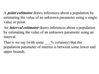
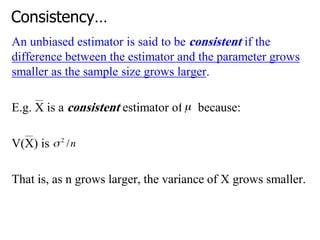
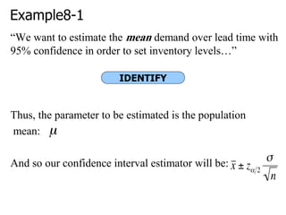
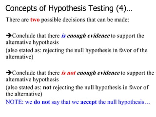
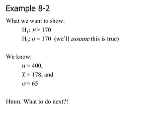
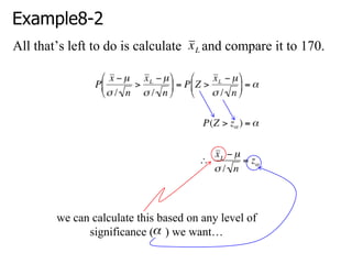
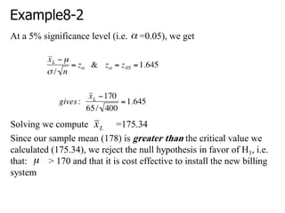
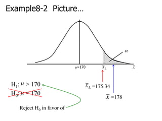
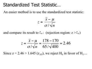
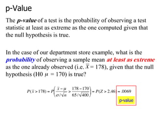
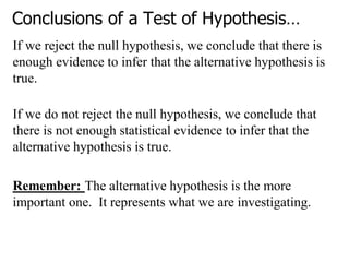
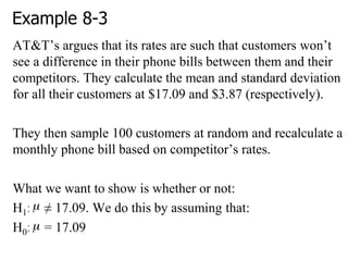
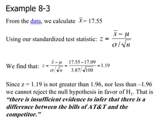
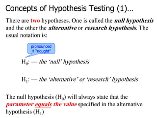
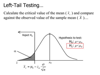
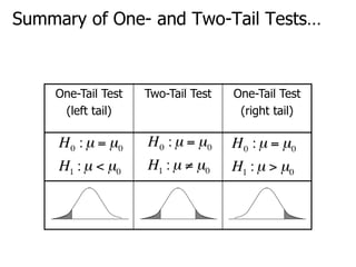
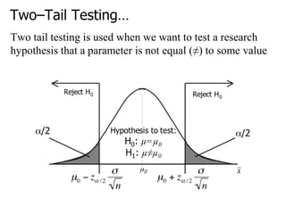
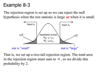
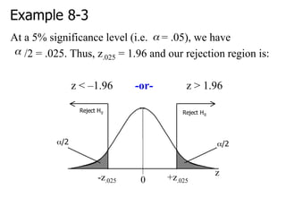
1. AT&T argues its rates are similar to competitors, with a mean of $17.09. It sampled 100 customers and recalculated bills based on competitors' rates. 2. The null hypothesis is that the mean is equal to AT&T's $17.09. The alternative hypothesis is that the mean is not equal to $17.09. 3. Using a two-tailed test at a 5% significance level, if the calculated p-value is less than 0.05 we would reject the null hypothesis, concluding the mean is likely not equal to $17.09.

1. TAIBAH UNIVERSITY
BADR
APPLIED COLLEGE
‫طيبة‬ ‫جامعة‬
‫ببدر‬ ‫التطبيقية‬ ‫الكلية‬
‫التدريس‬ ‫مكان‬
:
‫بدر‬
Statistics for Data Computation
Stat151
Coordinator: Dr.Mekki Noureddine
Chapter8:
Introduction to Estimation
Hypothesis Testing

2. Statistical Inference…
Statistical inference is the process by which we acquire
information and draw conclusions about populations from
samples.
In order to do inference, we require the skills and knowledge of descriptive statistics,
probability distributions, and sampling distributions.
Parameter
Population
Sample
Statistic
Inference
Data
Statistics
Information

3. 8-1-Estimation…
There are two types of inference: estimation and hypothesis
testing; estimation is introduced first.
The objective of estimation is to determine the approximate
value of a population parameter on the basis of a sample
statistic.
E.g., the sample mean ( ) is employed to estimate the
population mean ( ).

4. Estimation…
The objective of estimation is to determine the approximate
value of a population parameter on the basis of a sample
statistic.
There are two types of estimators:
Point Estimator
Interval Estimator

5. A point estimator draws inferences about a population by
estimating the value of an unknown parameter using a single
value or point.
An interval estimator draws inferences about a population
by estimating the value of an unknown parameter using an
interval.
That is we say (with some ___% certainty) that the
population parameter of interest is between some lower and
upper bounds.

6. Point & Interval Estimation…
For example, suppose we want to estimate the mean summer
income of a class of business students. For n=25 students,
is calculated to be 400 $/week.
point estimate interval estimate
An alternative statement is:
The mean income is between 380 and 420 $/week.

7. Qualities of Estimators…
Qualities desirable in estimators include unbiasedness,
consistency, and relative efficiency:
• An unbiased estimator of a population parameter is an
estimator whose expected value is equal to that parameter.
• An unbiased estimator is said to be consistent if the
difference between the estimator and the parameter grows
smaller as the sample size grows larger.
• If there are two unbiased estimators of a parameter, the
one whose variance is smaller is said to be relatively
efficient.

8. Unbiased Estimators…
An unbiased estimator of a population parameter is an
estimator whose expected value is equal to that parameter.
E.g. the sample mean X is an unbiased estimator of the
population mean , since:
E(X) =

9. Consistency…
An unbiased estimator is said to be consistent if the
difference between the estimator and the parameter grows
smaller as the sample size grows larger.
E.g. X is a consistent estimator of because:
V(X) is
That is, as n grows larger, the variance of X grows smaller.

10. Relative Efficiency…
If there are two unbiased estimators of a parameter, the one
whose variance is smaller is said to be relatively efficient.
E.g. both the the sample median and sample mean are
unbiased estimators of the population mean, however, the
sample median has a greater variance than the sample mean,
so we choose since it is relatively efficient when
compared to the sample median.

11. Estimating when is known…
We can calculate an interval estimator from a sampling
distribution, by:
Drawing a sample of size n from the population
Calculating its mean,
And, by the central limit theorem, we know that X is
normally (or approximately normally) distributed so…
…will have a standard normal (or approximately normal)
distribution.

12. Estimating when is known…
Looking at this in more detail…
Known, i.e. standard
normal distribution
Known, i.e. sample
mean
Unknown, i.e. we
want to estimate
the population mean
Known, i.e. the
number of items
sampled
Known, i.e. its
assumed we know
the population
standard deviation…

13. Confidence Interval Estimator for :
The probability 1– is called the confidence level.
lower confidence
limit (LCL)
upper confidence
limit (UCL)
Usually represented
with a “plus/minus”
( ± ) sign

14. Graphically…
…here is the confidence interval for :
width

15. Four commonly used confidence levels…
Confidence Level
 
cut & keep handy!

16. Example8-1
A computer company samples demand during lead time over
25 time periods:
Its is known that the standard deviation of demand over lead
time is 75 computers. We want to estimate the mean demand
over lead time with 95% confidence in order to set inventory
levels…
235 374 309 499 253
421 361 514 462 369
394 439 348 344 330
261 374 302 466 535
386 316 296 332 334

17. Example8-1
―We want to estimate the mean demand over lead time with
95% confidence in order to set inventory levels…‖
Thus, the parameter to be estimated is the population
mean:
And so our confidence interval estimator will be:
IDENTIFY

18. Example8-1
In order to use our confidence interval estimator, we need the
following pieces of data:
therefore:
The lower and upper confidence limits are 340.76 and 399.56.
370.16
1.96
75
n 25
Given
Calculated from the data…
CALCULATE

19. Example8-1
The estimation for the mean demand during lead time lies
between 340.76 and 399.56 — we can use this as input in
developing an inventory policy.
That is, we estimated that the mean demand during lead time
falls between 340.76 and 399.56, and this type of estimator
is correct 95% of the time. That also means that 5% of the
time the estimator will be incorrect.
INTERPRET

20. 8-2-Introduction To Hypothesis Testing…
Hypothesis testing is a procedure for making inferences
about a population.
Hypothesis testing allows us to determine whether enough
statistical evidence exists to conclude that a belief (i.e.
hypothesis) about a parameter is supported by the data.
Parameter
Population
Sample
Statistic
Inference

21. Concepts of Hypothesis Testing (1)…
There are two hypotheses. One is called the null hypothesis
and the other the alternative or research hypothesis. The
usual notation is:
H0: — the ‗null‘ hypothesis
H1: — the ‗alternative‘ or ‗research‘ hypothesis
The null hypothesis (H0) will always state that the
parameter equals the value specified in the alternative
hypothesis (H1)
pronounced
H “nought”

22. Concepts of Hypothesis Testing…
Consider Last Example (mean demand for computers
during assembly lead time) again. Rather than estimate the
mean demand, our operations manager wants to know
whether the mean is different from 350 units. We can
rephrase this request into a test of the hypothesis:
H0: = 350
Thus, our research hypothesis becomes:
H1: ≠ 350 This is what we are interested
in determining…

23. Concepts of Hypothesis Testing (2)…
The testing procedure begins with the assumption that the
null hypothesis is true.
Thus, until we have further statistical evidence, we will
assume:
H0: = 350 (assumed to be TRUE)

24. Concepts of Hypothesis Testing (3)…
The goal of the process is to determine whether there is
enough evidence to infer that the alternative hypothesis is
true.
That is, is there sufficient statistical information to determine
if this statement:
H1: ≠ 350, is true?
This is what we are interested
in determining…

25. Concepts of Hypothesis Testing (4)…
There are two possible decisions that can be made:
Conclude that there is enough evidence to support the
alternative hypothesis
(also stated as: rejecting the null hypothesis in favor of the
alternative)
Conclude that there is not enough evidence to support the
alternative hypothesis
(also stated as: not rejecting the null hypothesis in favor of
the alternative)
NOTE: we do not say that we accept the null hypothesis…

26. Concepts of Hypothesis Testing…
Once the null and alternative hypotheses are stated, the next
step is to randomly sample the population and calculate a
test statistic (in this example, the sample mean).
If the test statistic‘s value is inconsistent with the null
hypothesis we reject the null hypothesis and infer that the
alternative hypothesis is true.
For example, if we‘re trying to decide whether the mean is
not equal to 350, a large value of (say, 600) would provide
enough evidence. If is close to 350 (say, 355) we could
not say that this provides a great deal of evidence to infer
that the population mean is different than 350.

27. Concepts of Hypothesis Testing (5)…
Two possible errors can be made in any test:
A Type I error occurs when we reject a true null hypothesis
and
A Type II error occurs when we don‘t reject a false null
hypothesis.
There are probabilities associated with each type of error:
P(Type I error) =
P(Type II error ) =
Α is called the significance level.

28. Types of Errors…
A Type I error occurs when we reject a true null hypothesis
(i.e. Reject H0 when it is TRUE)
A Type II error occurs when we don’t reject a false null
hypothesis (i.e. Do NOT reject H0 when it is FALSE)
H0 T F
Reject I
Reject II

29. Types of Errors…
Back to our example, we would commit a Type I error if:
Reject H0 when it is TRUE
We reject H0 ( = 350) in favor of H1 ( ≠ 350) when in
fact the real value of is 350.
We would commit a Type II error in the case where:
Do NOT reject H0 when it is FALSE
We believe H0 is correct ( = 350), when in fact the real
value of is something other than 350.

30. Recap I…
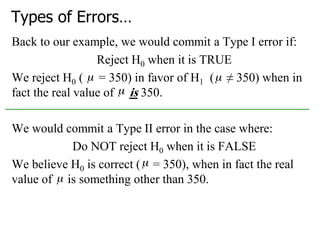
1) Two hypotheses: H0 & H1
2) ASSUME H0 is TRUE
3) GOAL: determine if there is enough evidence to infer that
H1 is TRUE
4) Two possible decisions:
Reject H0 in favor of H1
NOT Reject H0 in favor of H1
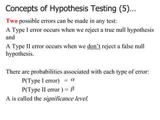
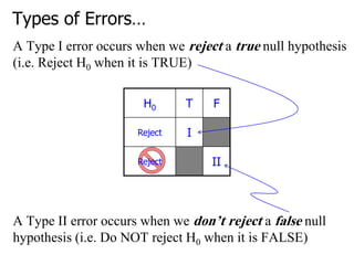
5) Two possible types of errors:
Type I: reject a true H0 [P(Type I)= ]
Type II: not reject a false H0 [P(Type II)= ]

31. Recap II…
The null hypothesis must specify a single value of the
parameter (e.g. =___)
Assume the null hypothesis is TRUE.
Sample from the population, and build a statistic related to
the parameter hypothesized (e.g. the sample mean, )
Compare the statistic with the value specified in the first
step

32. Example8-2
A department store manager determines that a new billing
system will be cost-effective only if the mean monthly
account is more than $170.
A random sample of 400 monthly accounts is drawn, for
which the sample mean is $178. The accounts are
approximately normally distributed with a standard deviation
of $65.
Can we conclude that the new system will be cost-
effective?

33. Example8-2
The system will be cost effective if the mean account
balance for all customers is greater than $170.
We express this belief as a our research hypothesis, that is:
H1: > 170 (this is what we want to determine)
Thus, our null hypothesis becomes:
H0: = 170 (this specifies a single value for the
parameter of interest)

34. Example 8-2
What we want to show:
H1: > 170
H0: = 170 (we‘ll assume this is true)
We know:
n = 400,
= 178, and
= 65
Hmm. What to do next?!

35. Example 8-2
To test our hypotheses, we can use two different approaches:
The rejection region approach (typically used when
computing statistics manually), and
The p-value approach (which is generally used with a
computer and statistical software).
We will explore both in turn…

36. Example8-2 Rejection Region…
The rejection region is a range of values such that if the test
statistic falls into that range, we decide to reject the null
hypothesis in favor of the alternative hypothesis.
is the critical value of to reject H0.

37. Example8-2
It seems reasonable to reject the null hypothesis in favor of
the alternative if the value of the sample mean is large
relative to 170, that is if > .
= P( > )
is also…
= P(rejecting H0 given that H0 is true)
= P(Type I error)

38. Example8-2
All that‘s left to do is calculate and compare it to 170.
we can calculate this based on any level of
significance ( ) we want…

39. Example8-2
At a 5% significance level (i.e. =0.05), we get
Solving we compute =175.34
Since our sample mean (178) is greater than the critical value we
calculated (175.34), we reject the null hypothesis in favor of H1, i.e.
that: > 170 and that it is cost effective to install the new billing
system

40. Example8-2 Picture…
=175.34
=178
H1: > 170
H0: = 170
Reject H0 in favor of

41. Standardized Test Statistic…
An easier method is to use the standardized test statistic:
and compare its result to : (rejection region: z > )
Since z = 2.46 > 1.645 (z.05), we reject H0 in favor of H1…

42. p-Value
The p-value of a test is the probability of observing a test
statistic at least as extreme as the one computed given that
the null hypothesis is true.
In the case of our department store example, what is the
probability of observing a sample mean at least as extreme
as the one already observed (i.e. = 178), given that the null
hypothesis (H0: = 170) is true?
p-value

43. Interpreting the p-value…
The smaller the p-value, the more statistical evidence exists
to support the alternative hypothesis.
•If the p-value is less than 1%, there is overwhelming
evidence that supports the alternative hypothesis.
•If the p-value is between 1% and 5%, there is a strong
evidence that supports the alternative hypothesis.
•If the p-value is between 5% and 10% there is a weak
evidence that supports the alternative hypothesis.
•If the p-value exceeds 10%, there is no evidence that
supports the alternative hypothesis.
We observe a p-value of .0069, hence there is
overwhelming evidence to support H1: > 170.

44. Interpreting the p-value…
Overwhelming Evidence
(Highly Significant)
Strong Evidence
(Significant)
Weak Evidence
(Not Significant)
No Evidence
(Not Significant)
0 .01 .05 .10
p=.0069

45. Interpreting the p-value…
Compare the p-value with the selected value of the
significance level:
If the p-value is less than , we judge the p-value to be
small enough to reject the null hypothesis.
If the p-value is greater than , we do not reject the null
hypothesis.
Since p-value = .0069 < = .05, we reject H0 in favor of
H1

46. Conclusions of a Test of Hypothesis…
If we reject the null hypothesis, we conclude that there is
enough evidence to infer that the alternative hypothesis is
true.
If we do not reject the null hypothesis, we conclude that
there is not enough statistical evidence to infer that the
alternative hypothesis is true.
Remember: The alternative hypothesis is the more
important one. It represents what we are investigating.

47. One– and Two–Tail Testing…
The department store example was a one tail test, because
the rejection region is located in only one tail of the
sampling distribution:
More correctly, this was an example of a right tail test.

48. One– and Two–Tail Testing…
The SSA Envelope example is a left tail test because the
rejection region was located in the left tail of the sampling
distribution.

49. Right-Tail Testing…
Calculate the critical value of the mean ( ) and compare
against the observed value of the sample mean ( )…

50. Left-Tail Testing…
Calculate the critical value of the mean ( ) and compare
against the observed value of the sample mean ( )…

51. Two–Tail Testing…
Two tail testing is used when we want to test a research
hypothesis that a parameter is not equal (≠) to some value

52. Example 8-3
AT&T‘s argues that its rates are such that customers won‘t
see a difference in their phone bills between them and their
competitors. They calculate the mean and standard deviation
for all their customers at $17.09 and $3.87 (respectively).
They then sample 100 customers at random and recalculate a
monthly phone bill based on competitor‘s rates.
What we want to show is whether or not:
H1: ≠ 17.09. We do this by assuming that:
H0: = 17.09

53. Example 8-3
The rejection region is set up so we can reject the null
hypothesis when the test statistic is large or when it is small.
That is, we set up a two-tail rejection region. The total area
in the rejection region must sum to , so we divide this
probability by 2.
stat is ―small‖ stat is ―large‖

54. Example 8-3
At a 5% significance level (i.e. = .05), we have
/2 = .025. Thus, z.025 = 1.96 and our rejection region is:
z < –1.96 -or- z > 1.96
z
-z.025 +z.025
0

55. Example 8-3
From the data, we calculate = 17.55
Using our standardized test statistic:
We find that:
Since z = 1.19 is not greater than 1.96, nor less than –1.96
we cannot reject the null hypothesis in favor of H1. That is
“there is insufficient evidence to infer that there is a
difference between the bills of AT&T and the
competitor.”

56. Summary of One- and Two-Tail Tests…
One-Tail Test
(left tail)
Two-Tail Test One-Tail Test
(right tail)