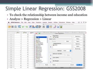
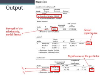
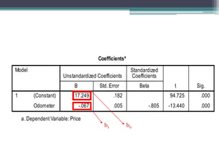
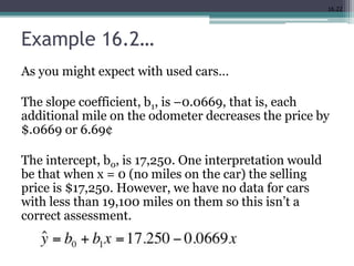
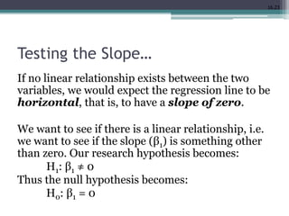
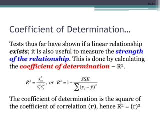
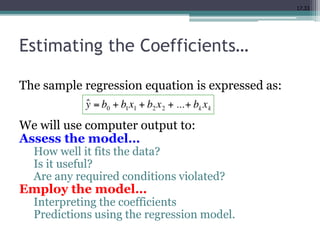
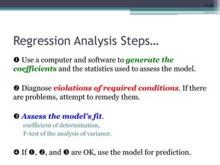
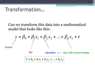
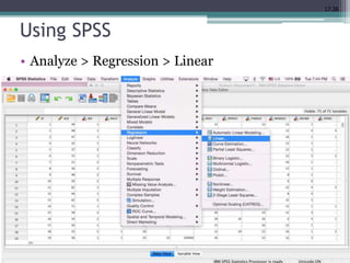
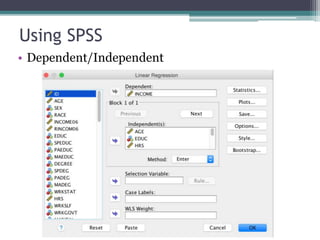
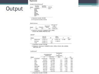
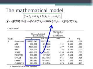
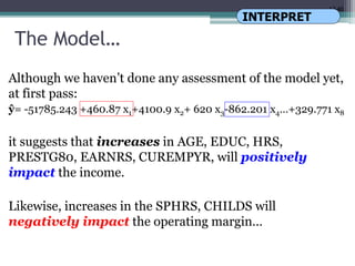
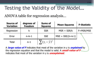
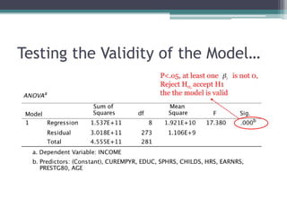
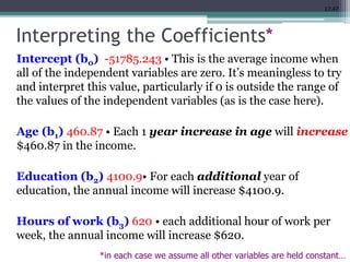
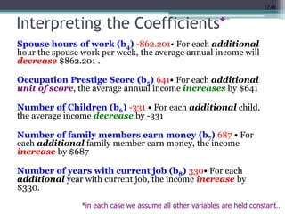
This document discusses quantitative research methods including correlation, simple linear regression, and multiple regression. It provides examples of how to conduct simple linear regression using SPSS to analyze the relationship between two variables and predict the dependent variable based on the independent variable. It then expands the discussion to multiple linear regression, using SPSS to analyze the relationships between multiple independent variables and one dependent variable. Key steps of assessing the model such as the coefficient of determination and F-test of ANOVA are also covered.

1. Quantitative Research Methods
Lecture 8
1. Correlation
2. Simple Linear Regression
3. Multiple Regression

2. Statistical analyses
• Group differences (nominal variable) on one interval
variable:
▫ T-tests (2 groups)
▫ ANOVA (3 or more groups)
 One factor: one way ANOVA
 Two factor: two way/factor ANOVA
• The relationship between two nominal variable:
▫ Chi-square test
• The relationship between two interval variable:
▫ Correlation, simple linear regression
• The relationship between more interval variable on one
interval variable
▫ Multiple regression

3. 16.3
Regression Analysis…
Objective: to analyze the relationship between
interval variables; regression analysis is the first
tool we will study.
Regression analysis is used to predict the value of one
variable (the dependent variable) on the basis of
other variables (the independent variables).
Dependent variable: denoted Y
Independent variables: denoted X1, X2, …, Xk

4. Regression
• Single Linear Regression
▫ one independent, one dependent
• Multiple Regression
▫ Multiple independent, one dependent
• Logistic Regression
• All dealing with interval variables

5. 16.5
Correlation Analysis…
If we are interested only in determining whether a
relationship exists, we employ correlation
analysis

6. Pearson Correlation Coefficient
•
17.6

7. SPSS steps: Example GSS2008
• To check the relationship between income and education
▫ Analyze > Correlation > Bivariate > check Pearson box

8. Output

9. Correlation and Regression
• Similarities:
▫ both dealing with two interval variables
• Differences:
▫ Correlation is not causation
▫ Regression indicates causal relationship
▫ Correlation can’t predict
▫ Regression can predict

10. 16.10
Simple Linear Regression Model…
A straight line model with one independent
variable is called a simple linear regression
model. Its is written as:
error variable
dependent
variable
independent
variable
y-intercept slope of the line

11. 16.11
Simple Linear Regression Model…
Note that both and are population
parameters which are usually unknown and
hence estimated from the data.
y
x
run
rise
=slope (=rise/run)
=y-intercept

12. 16.12
Estimating the Coefficients…
In much the same way we base estimates of µ on x , we
estimate β0 using b0 and β1 using b1, the y-intercept
and slope (respectively) of the least squares or
regression line given by:
(Recall: this is an application of the least squares
method and it produces a straight line that
minimizes the sum of the squared differences
between the points and the line)

13. Simple Linear Regression: GSS2008
• To check the relationship between income and education
• Analyze > Regression > Linear

14. Output
b1
b0
Model
significance
Strength of the
relationship,
model fitness
Significance of the predictor

15. 16.15
Example 16.1
The annual bonuses ($1,000s) of six employees with different
years of experience were recorded as follows. We wish to
determine the straight line relationship between annual bonus
and years of experience.
Years of experience x 1 2 3 4 5 6
Annual bonus y 6 1 9 5 17 12
Xm16-01

16. 16.16
Least Squares Line…
these differences are
called residuals
Example 16.1

17. 16.17
Example 16.2…
Car dealers across North America use the "Red Book" to
help them determine the value of used cars that their
customers trade in when purchasing new cars.
The book, which is published monthly, lists the trade-in
values for all basic models of cars.
It provides alternative values for each car model according
to its condition and optional features.
The values are determined on the basis of the average paid
at recent used-car auctions, the source of supply for many
used-car dealers.

18. 16.18
Example 16.2…
However, the Red Book does not indicate the value
determined by the odometer reading, despite the fact that a
critical factor for used-car buyers is how far the car has
been driven.
To examine this issue, a used-car dealer randomly selected
100 three-year old Toyota Camrys that were sold at auction
during the past month.
The dealer recorded the price ($1,000) and the number of
miles (thousands) on the odometer. (Xm16-02).
The dealer wants to find the regression line.

19. 16.19
Using SPSS
Analyze > Regression > Linear
Simple Linear Regression
Steps: Analyze > Regression > Linear

20. 16.20
Output
Check three tables:
R2 strength of the linear relationship
Model
significance

21. b1 b0

22. 16.22
Example 16.2…
As you might expect with used cars…
The slope coefficient, b1, is –0.0669, that is, each
additional mile on the odometer decreases the price by
$.0669 or 6.69¢
The intercept, b0, is 17,250. One interpretation would
be that when x = 0 (no miles on the car) the selling
price is $17,250. However, we have no data for cars
with less than 19,100 miles on them so this isn’t a
correct assessment.

23. 16.23
Testing the Slope…
If no linear relationship exists between the two
variables, we would expect the regression line to be
horizontal, that is, to have a slope of zero.
We want to see if there is a linear relationship, i.e.
we want to see if the slope (β1) is something other
than zero. Our research hypothesis becomes:
H1: β1 ≠ 0
Thus the null hypothesis becomes:
H0: β1 = 0

24. 16.24
Coefficient of Determination…
Tests thus far have shown if a linear relationship
exists; it is also useful to measure the strength
of the relationship. This is done by calculating
the coefficient of determination – R2.
The coefficient of determination is the square of
the coefficient of correlation (r), hence R2 = (r)2

25. 16.25
Coefficient of Determination…
As we did with analysis of variance, we can partition
the variation in y into two parts:
Variation in y = SSE + SSR
SSE – Sum of Squares Error – measures the amount of
variation in y that remains unexplained (i.e. due to
error)
SSR – Sum of Squares Regression – measures the
amount of variation in y explained by variation in the
independent variable x.

26. 16.26
Coefficient of Determination
R2 has a value of .6483. This means 64.83% of the variation
in the auction selling prices (y) is explained by the variation
in the odometer readings (x). The remaining 35.17% is
unexplained, i.e. due to error.
Unlike the value of a test statistic, the coefficient of
determination does not have a critical value that
enables us to draw conclusions.
In general the higher the value of R2, the better the model
fits the data.
R2 = 1: Perfect match between the line and the data points.
R2 = 0: There are no linear relationship between x and y.

27. From simple linear regression to
multiple regression
• Simple linear regression
Education
Income

28. 17.28
Multiple Regression…
The simple linear regression model was used to
analyze how one interval variable (the dependent
variable y) is related to one other interval variable (the
independent variable x).
Multiple regression allows for any number of
independent variables.
We expect to develop models that fit the data better
than would a simple linear regression model.

29. Multiple regression
Variable A
Variable D
Variable B
Variable C

30. Multiple regression
Age
Income
Education
Number of
Family member
earn money
Number of
Children
Year
With current
employer
Occupation
Prestige score
Work hours

31. Example: GSS2008
• How is income affected by
▫ Age (AGE)
▫ Education (EDUC)
▫ Work hours (HRS)
▫ Spouse work hours (SPHRS)
▫ Occupation prestige score (PRESTG80)
▫ Number of children (CHILDS)
▫ Number of family members earn money (EARNS)
▫ Years with current employer (CUREMPYR)

32. 17.32
The Model…
We now assume we have k independent variables potentially
related to the one dependent variable. This relationship is
represented in this first order linear equation:
In the one variable, two dimensional case we drew a regression
line; here we imagine a response surface.
error variable
dependent
variable
independent variables
coefficients

33. 17.33
Estimating the Coefficients…
The sample regression equation is expressed as:
We will use computer output to:
Assess the model…
How well it fits the data?
Is it useful?
Are any required conditions violated?
Employ the model…
Interpreting the coefficients
Predictions using the regression model.

34. 17.34
Regression Analysis Steps…
u Use a computer and software to generate the
coefficients and the statistics used to assess the model.
v Diagnose violations of required conditions. If there
are problems, attempt to remedy them.
w Assess the model’s fit.
coefficient of determination,
F-test of the analysis of variance.
x If u, v, and w are OK, use the model for prediction.

35. 17.35
Transformation…
Can we transform this data into a mathematical
model that looks like this:
income
education Year with current employ…age

36. 17.36
Using SPSS
• Analyze > Regression > Linear

37. Using SPSS
• Dependent/Independent

38. Output

39. The mathematical model
ŷ= -51785.243 +460.87 x1+4100.9 x2+…+329.771 x8

40. 17.40
The Model…
Although we haven’t done any assessment of the model yet,
at first pass:
ŷ= -51785.243 +460.87 x1+4100.9 x2+ 620 x3-862.201 x4…+329.771 x8
it suggests that increases in AGE, EDUC, HRS,
PRESTG80, EARNRS, CUREMPYR, will positively
impact the income.
Likewise, increases in the SPHRS, CHILDS will
negatively impact the operating margin…
INTERPRET

41. 17.41
Model Assessment…
We will assess the model in two ways:
Coefficient of determination, and
F-test of the analysis of variance.

42. 17.42
Coefficient of Determination…
• Again, the coefficient of determination is defined
as:
This means that 33.7% of the variation in income is
explained by the six independent variables, but
66.3% remains unexplained.

43. 17.43
Adjusted R2 value…
The adjusted” R2 is:
the coefficient of determination adjusted
for the number of explanatory variables.
It takes into account the sample size n, and k, the
number of independent variables, and is given by:

44. 17.44
Testing the Validity of the Model…
In a multiple regression model (i.e. more than one
independent variable), we utilize an analysis of
variance technique to test the overall validity of the
model. Here’s the idea:
H0:
H1: At least one is not equal to zero.
If the null hypothesis is true, none of the independent
variables is linearly related to y, and so the model is
invalid.
If at least one is not equal to 0, the model does have
some validity.

45. 17.45
Testing the Validity of the Model…
ANOVA table for regression analysis…
Source of
Variation
degrees of
freedom
Sums of
Squares
Mean Squares F-Statistic
Regression k SSR MSR = SSR/k F=MSR/MSE
Error n–k–1 SSE MSE = SSE/(n–k-1)
Total n–1
A large value of F indicates that most of the variation in y is explained by
the regression equation and that the model is valid. A small value of F
indicates that most of the variation in y is unexplained.

46. Testing the Validity of the Model…
P<.o5, at least one is not 0,
Reject H0, accept H1
the the model is valid

47. 17.47
Interpreting the Coefficients*
Intercept (b0) -51785.243 • This is the average income when
all of the independent variables are zero. It’s meaningless to try
and interpret this value, particularly if 0 is outside the range of
the values of the independent variables (as is the case here).
Age (b1) 460.87 • Each 1 year increase in age will increase
$460.87 in the income.
Education (b2) 4100.9• For each additional year of
education, the annual income will increase $4100.9.
Hours of work (b3) 620 • each additional hour of work per
week, the annual income will increase $620.
*in each case we assume all other variables are held constant…

48. 17.48
Interpreting the Coefficients*
Spouse hours of work (b4) -862.201• For each additional
hour the spouse work per week, the average annual income will
decrease $862.201 .
Occupation Prestige Score (b5) 641• For each additional
unit of score, the average annual income increases by $641
Number of Children (b6) -331 • For each additional child,
the average income decrease by -331
Number of family members earn money (b7) 687 • For
each additional family member earn money, the income
increase by $687
Number of years with current job (b8) 330• For each
additional year with current job, the income increase by
$330.
*in each case we assume all other variables are held constant…

49. 17.49
Testing the Coefficients…
For each independent variable, we can test to
determine whether there is enough evidence of a linear
relationship between it and the dependent variable for
the entire population…
H0: = 0
H1: ≠ 0
(for i = 1, 2, …, k) and using:
as our test statistic (with n–k–1 degrees of freedom).

50. 17.50
Testing the Coefficients
We can use SPSS output to quickly test each of the
8 coefficients in our model…
Thus, EDUC, HRS, SPHRS, PRESTG80, are linearly related to the
operating margin. There is no evidence to infer that AGE, CHILDS,
EARNS, CUREMPYR are linearly related to operating margin.

51. Weekly assignment
• Read chapter 14-17
• Assignment Due Tuesday Nov. 13th, on blackboard
▫ P533 X14.18 use data Xr 14.18 add post hoc test in
interpretation of the data.
▫ P556 14.96 use data Xr14.64
▫ P570 14.109 use data Xr14.77
▫ P610 15.42 use data Xr15.38