Downloaded 432 times


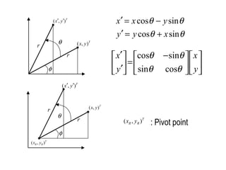

![rotation
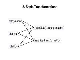
scaling
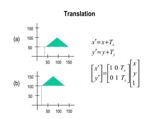
translation
perspective transform
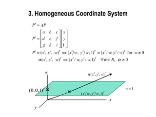
P 'P
T '
where
' [ ', ', '] ,
[ , , ] .
T
T
P TP
P x y w
P x y w
=
=
=
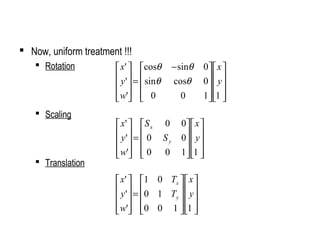
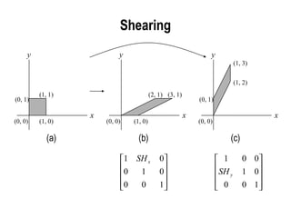
2D Transformation Matrices
=
ihg
fed
cba
T
X 'X](https://image.slidesharecdn.com/cs580-052dtransformations-140720144044-phpapp01/85/2d-3D-transformations-in-computer-graphics-Computer-graphics-Tutorials-21-320.jpg)
![]][]...[[][
][
]][]...[['
12
12
TTTT
PT
PTTTP
n
n
=
=
=
composite transformation matrix
HomeworkHomework
4. Composite Transformations](https://image.slidesharecdn.com/cs580-052dtransformations-140720144044-phpapp01/85/2d-3D-transformations-in-computer-graphics-Computer-graphics-Tutorials-23-320.jpg)
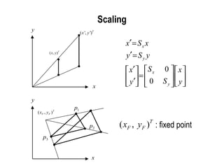
![( , )T
F Fx y
(a) Original position of
object and fixed point
(b) Translate object so that
fixed point (xF, yF) is at origin
(c) Scale object with
respect to origin
(d) Translate object so that
fixed point is returned to position (xF, yF)T
( , )T
F Fx y
][ rT
][ cS 1
][ −
rT](https://image.slidesharecdn.com/cs580-052dtransformations-140720144044-phpapp01/85/2d-3D-transformations-in-computer-graphics-Computer-graphics-Tutorials-24-320.jpg)
![( , )T
R Rx y
(a) Original position of
object and pivot point
(b) Translation of object so that
the pivot point (xR, yR) is at origin
(c) Rotation about origin (d) Translation of object so that
the pivot point is returned to
position (xR, yR)T
( , )T
R Rx y
][ rT
][ tR 1
][ −
rT](https://image.slidesharecdn.com/cs580-052dtransformations-140720144044-phpapp01/85/2d-3D-transformations-in-computer-graphics-Computer-graphics-Tutorials-25-320.jpg)
![x
y
θ
Sy
Sx
[Rt]-1
[Sc][Rt]](https://image.slidesharecdn.com/cs580-052dtransformations-140720144044-phpapp01/85/2d-3D-transformations-in-computer-graphics-Computer-graphics-Tutorials-26-320.jpg)
![Final
Position
Final
Position
(a) [Rt][Tr] (b) [Tr][Rt]](https://image.slidesharecdn.com/cs580-052dtransformations-140720144044-phpapp01/85/2d-3D-transformations-in-computer-graphics-Computer-graphics-Tutorials-29-320.jpg)
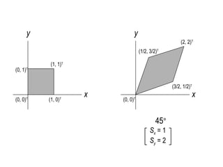
![45°
[Rt] [Rf
x
]
45°
[Rt]-1
Reflection about y = x](https://image.slidesharecdn.com/cs580-052dtransformations-140720144044-phpapp01/85/2d-3D-transformations-in-computer-graphics-Computer-graphics-Tutorials-32-320.jpg)
This document discusses the Daroko blog, which provides real-world applications of various IT skills. It encourages readers to not just learn computer graphics and other topics but to apply them in business contexts. The blog covers topics like computer graphics, networking, programming, IT jobs, technology news, blogging, website building, and IT companies. It aims to help readers gain practical experience applying their IT knowledge. Readers are instructed to search "Daroko blog" online to access resources on various IT subjects and their business applications.