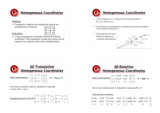
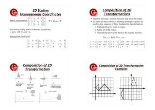
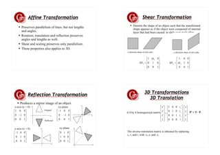
The document provides an overview of 2D and 3D geometric transformations including translation, rotation, scaling, and homogeneous coordinates. It then describes 2D translation, rotation, and scaling transformations through equations, matrix representations, and examples. Key points covered include: - Translating an object by adding translation distances tx and ty to the original coordinates - Rotating an object using a rotation angle θ and pivot point coordinates - Scaling an object by multiplying coordinates by scaling factors sx and sy - Representing transformations using homogeneous coordinates and transformation matrices - Composing multiple transformations through matrix multiplication

1. Overview
● 2D and 3D
– Translation
– Rotation
– Scaling
● Homogeneous Coordinates
● Coordinate Systems
Geometric Transformations
2D Translation
• Repositioning an object along a straight line path from one coordinate
location to another.
● Adding translation distances, tx and ty, to the original coordinate
position.
● Rigid-body transformation:
– Moves object without deformation.
y
x t
y
y
t
x
x +
=
+
= '
'
x
y
x
y
Before translation After translation
,
'
'
⎥
⎦
⎤
⎢
⎣
⎡
+
⎥
⎦
⎤
⎢
⎣
⎡
=
⎥
⎦
⎤
⎢
⎣
⎡
y
x
t
t
y
x
y
x
Matrix form:
P' = P + T
Geometric Transformations
2D Rotation
• Repositioning an object along a circular path.
• Need a rotation angle θ and the position (xr, yr) of the pivot point which
the object is to be rotated about.
• Positive rotation angles give counterclockwise rotation and negative
angles give clockwise rotation.
x
y
x
y
Before rotation After rotation
Rotation equation about origin:
θ
φ
θ
φ
θ
φ
θ
φ
θ
φ
θ
φ
cos
sin
sin
cos
)
sin(
'
sin
sin
cos
cos
)
cos(
'
r
r
r
y
r
r
r
x
+
=
+
=
−
=
+
=
Geometric Transformations
2D Rotation
Original polar coordinates:
θ
φ sin
cos r
y
r
x =
=
After substitution:
θ
θ
θ
θ
cos
sin
'
sin
cos
'
y
x
y
y
x
x
+
=
−
=
Matrix form:
,
cos
sin
sin
cos
'
'
⎥
⎦
⎤
⎢
⎣
⎡
⋅
⎥
⎦
⎤
⎢
⎣
⎡ −
=
⎥
⎦
⎤
⎢
⎣
⎡
y
x
y
x
θ
θ
θ
θ
Rotation about origin:
P' = R · P

2. Geometric Transformations
2D Rotation
After substitution:
( ) ( )
( ) ( ) θ
θ
θ
θ
cos
sin
'
sin
cos
'
r
r
r
r
r
r
y
y
x
x
y
y
y
y
x
x
x
x
−
+
−
+
=
−
−
−
+
=
Rotation about an arbitrary pivot point:
Geometric Transformations
2D Rotation
● Rigid-body transformation
● A line is rotated by applying the rotation equation to
each of the line endpoints and redrawing the line
between the tow endpoints.
● Polygons are rotated by moving each vertex through
the specified rotation angle and then redraw.
● Curves are rotated by repositioning the defining
points and redrawing the curve.
• Alters the size of an object.
• An object is scaled by multiplying the coordinates (x,y) of each vertex
by a scaling factor sx and sy.
• sx and sy can be any positive value.
– Values < 1 reduces the size of the object.
– Values > 1 produces and enlargement.
– If sx and sy is 1, then the size is unchanged.
y
x s
y
y
s
x
x ⋅
=
⋅
= '
'
x
y
x
y
Before scaling After scaling
,
0
0
'
'
⎥
⎦
⎤
⎢
⎣
⎡
⎥
⎦
⎤
⎢
⎣
⎡
=
⎥
⎦
⎤
⎢
⎣
⎡
y
x
s
s
y
x
y
x
Matrix form:
P' = S · P
Geometric Transformations
2D Scaling
• Uniform scaling:
– sx and sy have the same value.
• Differential scaling:
– Unequal values of sx and sy.
• Scaling values < 1 moves the object closer to the origin.
• Scaling values > 1 moves the object further away from the origin.
• Fixed point:
– To control the location after scaling.
– Coordinates for the fixed point (xf, yf) can be any vertices,
centroids or any other position.
– xf(1-sx) and yf(1-sy) are constants for all
points in the object.
)
1
(
'
)
1
(
'
y
f
y
x
f
x
s
y
s
y
y
s
x
s
x
x
−
+
⋅
=
−
+
⋅
=
Geometric Transformations
2D Scaling

3. Homogeneous Coordinates
Problem:
● Translation is addition and scaling and rotation are
multiplication of matrices.
Solved by:
● Using homogeneous coordinates instead of cartesian
coordinates. Then translation, scaling and rotation can be
expressed in a general matrix form (multiplication).
P' = P + T
P' = R · P
P' = S · P
Homogeneous Coordinates
• A 2D coordinate P1(x1,y1) lying in 3D can be represented as
P(x,y,z) = P(hx1,hy1,h).
• Given P(m,n,h) in homogeneous coordinates the cartesian coordinates
can be found by P(m/h,n/h,1).
• Each point can have many
different homogeneous
coordinate representations.
2D Translation
Homogeneous Coordinates
Matrix representation: ,
1
1
0
0
1
0
0
1
1
'
'
⎥
⎥
⎥
⎦
⎤
⎢
⎢
⎢
⎣
⎡
⋅
⎥
⎥
⎥
⎦
⎤
⎢
⎢
⎢
⎣
⎡
=
⎥
⎥
⎥
⎦
⎤
⎢
⎢
⎢
⎣
⎡
y
x
t
t
y
x
y
x
P' = T(tx,ty) · P
The inverse translation matrix is obtained by replacing
tx and ty with -tx and -ty.
⎥
⎥
⎥
⎦
⎤
⎢
⎢
⎢
⎣
⎡
+
+
=
⎥
⎥
⎥
⎦
⎤
⎢
⎢
⎢
⎣
⎡
⋅
⎥
⎥
⎥
⎦
⎤
⎢
⎢
⎢
⎣
⎡
1
0
0
1
0
0
1
1
0
0
1
0
0
1
1
0
0
1
0
0
1
2
1
2
1
1
1
2
2
y
y
x
x
y
x
y
x
t
t
t
t
t
t
t
t
Translating from P to P' to P'':
2D Rotation
Homogeneous Coordinates
Matrix representation: ,
1
1
0
0
0
cos
sin
0
sin
cos
1
'
'
⎥
⎥
⎥
⎦
⎤
⎢
⎢
⎢
⎣
⎡
⋅
⎥
⎥
⎥
⎦
⎤
⎢
⎢
⎢
⎣
⎡ −
=
⎥
⎥
⎥
⎦
⎤
⎢
⎢
⎢
⎣
⎡
y
x
y
x
θ
θ
θ
θ
P' = R(θ) · P
The inverse rotation matrix is obtained by replacing θ by -θ.
( ) ( )
( ) ( )
⎥
⎥
⎥
⎦
⎤
⎢
⎢
⎢
⎣
⎡
+
+
+
−
+
=
⎥
⎥
⎥
⎦
⎤
⎢
⎢
⎢
⎣
⎡ −
⋅
⎥
⎥
⎥
⎦
⎤
⎢
⎢
⎢
⎣
⎡ −
1
0
0
0
cos
sin
0
sin
cos
1
0
0
0
cos
sin
0
sin
cos
1
0
0
0
cos
sin
0
sin
cos
2
1
2
1
2
1
2
1
1
1
1
1
2
2
2
2
θ
θ
θ
θ
θ
θ
θ
θ
θ
θ
θ
θ
θ
θ
θ
θ
Two successive rotations:

4. 2D Scaling
Homogeneous Coordinates
Matrix representation: ,
1
1
0
0
0
0
0
0
1
'
'
⎥
⎥
⎥
⎦
⎤
⎢
⎢
⎢
⎣
⎡
⋅
⎥
⎥
⎥
⎦
⎤
⎢
⎢
⎢
⎣
⎡
=
⎥
⎥
⎥
⎦
⎤
⎢
⎢
⎢
⎣
⎡
y
x
s
s
y
x
y
x
P' = S(sx,sy) · P
The inverse scaling matrix is obtained by replacing
sx and sy with 1/sx and 1/sy.
⎥
⎥
⎥
⎦
⎤
⎢
⎢
⎢
⎣
⎡
⋅
⋅
=
⎥
⎥
⎥
⎦
⎤
⎢
⎢
⎢
⎣
⎡
⋅
⎥
⎥
⎥
⎦
⎤
⎢
⎢
⎢
⎣
⎡
1
0
0
0
0
0
0
1
0
0
0
0
0
0
1
0
0
0
0
0
0
2
1
2
1
1
1
2
2
x
x
x
x
y
x
y
x
s
s
s
s
s
s
s
s
Scaling from P to P' to P'':
Composition of 2D
Transformations
● OpenGL provides a rotation function only about the origin.
● To rotate an object about an arbitrary point (pivot point) we
need to do a sequence of three fundamental transformations.
1. Translate the pivot point to origin.
2. Rotate about the origin.
3. Translate the pivot point back to the original position.
( )
( )
⎥
⎥
⎥
⎦
⎤
⎢
⎢
⎢
⎣
⎡
−
−
+
−
−
=
⎥
⎥
⎥
⎦
⎤
⎢
⎢
⎢
⎣
⎡
−
−
⋅
⎥
⎥
⎥
⎦
⎤
⎢
⎢
⎢
⎣
⎡ −
⋅
⎥
⎥
⎥
⎦
⎤
⎢
⎢
⎢
⎣
⎡
1
0
0
sin
cos
1
cos
sin
sin
cos
1
sin
cos
1
0
0
1
0
0
1
1
0
0
0
cos
sin
0
sin
cos
1
0
0
1
0
0
1
1
1
1
1
1
1
1
1
θ
θ
θ
θ
θ
θ
θ
θ
θ
θ
θ
θ
x
y
y
x
y
x
y
x
T(x1, y1) · R(θ) · T(-x1, -y1) =
Composition of 2D
Transformation
Composition of 2D Transformation
Examples

5. Affine Transformation
● Preserves parallelism of lines, but not lengths
and angles.
● Rotation, translation and reflection preserves
angles and lengths as well.
● Shear and scaling preserves only parallelism.
● These properties also applies to 3D.
Shear Transformation
● Distorts the shape of an object such that the transformed
shape appears as if the object were composed of internal
layer that had been caused to slide over each other.
x-direction shear of unit cube. y-direction shear of unit cube.
⎥
⎥
⎥
⎦
⎤
⎢
⎢
⎢
⎣
⎡
=
⎥
⎥
⎥
⎦
⎤
⎢
⎢
⎢
⎣
⎡
=
1
0
0
0
1
0
0
1
,
1
0
0
0
1
0
0
1
y
y
x
x sh
SH
sh
SH
Reflection Transformation
● Produces a mirror image of an object.
⎥
⎥
⎥
⎦
⎤
⎢
⎢
⎢
⎣
⎡
−
1
0
0
0
1
0
0
0
1
⎥
⎥
⎥
⎦
⎤
⎢
⎢
⎢
⎣
⎡
1
0
0
0
0
1
0
1
0
⎥
⎥
⎥
⎦
⎤
⎢
⎢
⎢
⎣
⎡−
1
0
0
0
1
0
0
0
1
⎥
⎥
⎥
⎦
⎤
⎢
⎢
⎢
⎣
⎡
−
−
1
0
0
0
1
0
0
0
1
x-axis (y = 0)
y-axis (x = 0)
xy-plane
xy-plane
Original
Reflected
x
x
y
y
x
x
y
y
3D Transformations
3D Translation
,
1
1
0
0
0
1
0
0
0
1
0
0
0
1
1
'
'
'
⎥
⎥
⎥
⎥
⎦
⎤
⎢
⎢
⎢
⎢
⎣
⎡
⋅
⎥
⎥
⎥
⎥
⎦
⎤
⎢
⎢
⎢
⎢
⎣
⎡
=
⎥
⎥
⎥
⎥
⎦
⎤
⎢
⎢
⎢
⎢
⎣
⎡
z
y
x
t
t
t
z
y
x
z
y
x
P' = T · P
A 4 by 4 homogenized matrix
The inverse translation matrix is obtained by replacing
tx, ty and tz with -tx,-ty and -tz.

6. 3D Transformation
3D Translation
● Each of the defining points are translated.
● If the object is a polygon, each vertex of the
polygon is translated.
(x',y',z')
(x,y,z)
T = (tx, ty, tz) T = (tx, ty, tz)
3D Transformations
3D Scaling
,
1
1
0
0
0
0
0
0
0
0
0
0
0
0
1
'
'
'
⎥
⎥
⎥
⎥
⎦
⎤
⎢
⎢
⎢
⎢
⎣
⎡
⋅
⎥
⎥
⎥
⎥
⎦
⎤
⎢
⎢
⎢
⎢
⎣
⎡
=
⎥
⎥
⎥
⎥
⎦
⎤
⎢
⎢
⎢
⎢
⎣
⎡
z
y
x
s
s
s
z
y
x
z
y
x
P' = S ·P
A 4 by 4 homogenized matrix
The inverse scaling matrix is obtained by replacing
sx, sy and sz with 1/sx,1/sy and 1/sz.
3D Transformation
3D Scaling
Scaling with respect to a fixed position
( )
( )
( )
⎥
⎥
⎥
⎥
⎦
⎤
⎢
⎢
⎢
⎢
⎣
⎡
−
−
−
=
−
−
−
⋅
⋅
1
0
0
0
1
0
0
1
0
0
1
0
0
)
,
,
(
T
)
,
,
(
S
)
,
,
(
T
f
z
z
f
y
y
f
x
x
f
f
f
z
y
x
f
f
f
z
s
s
y
s
s
x
s
s
z
y
x
s
s
s
z
y
x
x
y
z x
y
z x
y
z x
y
z
(xf,yf,zf) (xf,yf,zf)
(xf,yf,zf) (xf,yf,zf)
3D Transformation
3D Rotation
⎥
⎥
⎥
⎥
⎦
⎤
⎢
⎢
⎢
⎢
⎣
⎡ −
1
0
0
0
0
1
0
0
0
0
cos
sin
0
0
sin
cos
θ
θ
θ
θ
x
y
z
x
y
z
x
y
z
⎥
⎥
⎥
⎥
⎦
⎤
⎢
⎢
⎢
⎢
⎣
⎡
−
1
0
0
0
0
cos
sin
0
0
sin
cos
0
0
0
0
1
θ
θ
θ
θ
⎥
⎥
⎥
⎥
⎦
⎤
⎢
⎢
⎢
⎢
⎣
⎡
−
1
0
0
0
0
cos
0
sin
0
0
1
0
0
sin
0
cos
θ
θ
θ
θ
P' = Rz(θ) ·P P' = Rx(θ) ·P
P' = Ry(θ) ·P
Rotation about z-axis Rotation about x-axis
Rotation about y-axis

7. Geometric Transformation
⎥
⎥
⎥
⎥
⎦
⎤
⎢
⎢
⎢
⎢
⎣
⎡
⎥
⎥
⎥
⎦
⎤
⎢
⎢
⎢
⎣
⎡
1
0
0
0
1
0
0 33
32
31
23
22
21
13
12
11
22
21
12
11
z
y
x
y
x
t
r
r
r
t
r
r
r
t
r
r
r
or
t
r
r
t
r
r
A transformation matrix of the form: (translation and rotation)
is called special orthogonal.
It preserves angles and length.
The inverse is the transpose.
Each row vector in the matrix has 3 properties:
1. Each is a unit vector
2. Each is perpendicular to the other
3. The first and second vector will be rotated by R(θ)
to lie on the positive x and y axes, respectively.
Composition of 3D
Transformation
Initial position Final position
x
z
y
P1
P3
P2
x
z
y
P1
P3
P2
Two ways to achieve the transformation:
1. Compose the transformation T, Rx, Ry, Rz.
2. Using the properties of the orthogonal matrix.
Composition of 3D
Transformation
Done the same way as 2D composition.
1. Translate P1 to the origin
2. Rotate about the y-axis (P1,P2 lies in the (y,z) plane)
3. Rotate about the x-axis (P1,P2 lies on the z-axis)
4. Rotate about the z-axis (P1,P3 lies in the (y,z) plane)
The composite matrix will be
( ) ( ) ( ) )
,
,
(
90 1
1
1 z
y
x
T
R
R
R y
x
z −
−
−
⋅
−
⋅
⋅ θ
φ
α
Composition of 3D
Transformation
Rz will rotate into z-axis.
Create the rotation matrix by using cross product.
[ ]
2
1
2
1
3
2
1
P
P
P
P
r
r
r
R
T
z
z
z
z =
=
Rx will rotate into x-axis.
[ ]
2
1
3
1
2
1
3
1
3
2
1
P
P
P
P
P
P
P
P
r
r
r
R
T
x
x
x
x
×
×
=
=
Ry will rotate into y-axis.
[ ]
x
z
x
z
T
y
y
y
y
R
R
R
R
r
r
r
R
×
×
=
= 3
2
1
T
R
z
y
x
T
r
r
r
r
r
r
r
r
r
z
z
z
y
y
y
x
x
x
⋅
=
−
−
−
⋅
⎥
⎥
⎥
⎥
⎦
⎤
⎢
⎢
⎢
⎢
⎣
⎡
)
,
,
(
1
0
0
0
0
0
0
1
1
1
3
2
1
3
2
1
3
2
1
Composite
Matrix

8. Coordinate Systems
Right handed:
x
z
y
Positive rotation gives
counterclockwise rotation
Left handed:
x
z
y
Positive rotation is clockwise