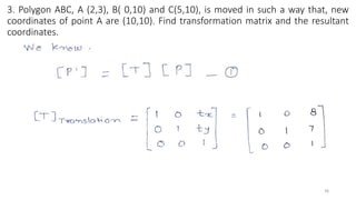
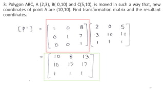
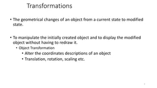
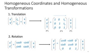
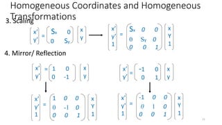
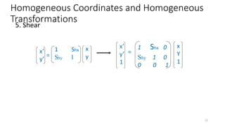
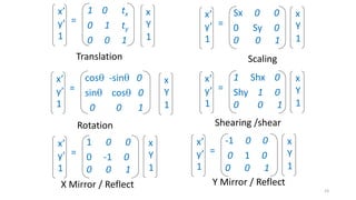
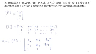
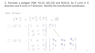
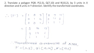
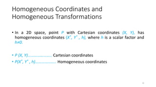
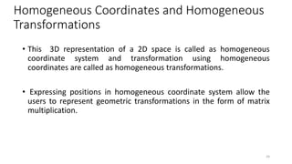
1. The document discusses various 2D transformations including translation, rotation, scaling, reflection, shearing, and their representation using homogeneous coordinates and homogeneous transformations. All transformations can be represented as matrix multiplication using homogeneous coordinates. 2. Homogeneous coordinates allow geometric transformations to be expressed as matrix multiplications, enabling efficient concatenation of multiple transformations. Any 2D point (x,y) can be represented as a 3D homogeneous coordinate (x,y,1). 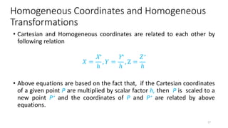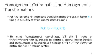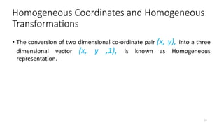3. Common transformations like translation, rotation, scaling, etc. that were previously represented using vector addition can now be uniformly represented using matrix multiplications in homogeneous coordinates. This allows multiple transformations to be applied sequentially with a single matrix multiplication.

1. 1
2-D
Transformations

2. Transformations
• The geometrical changes of an object from a current state to modified
state.
• To manipulate the initially created object and to display the modified
object without having to redraw it.
• Object Transformation
• Alter the coordinates descriptions of an object
• Translation, rotation, scaling etc.
2

3. 2D Transformations
• Translation
• Rotation
• Scaling
• Mirror / Reflect
• Shearing /shear
3

4. • A translation moves all points in an
object along the same straight-line
path to new positions.
• The path is represented by a vector,
called the translation or shift vector.
p'x = tx + px
p'y = ty + py
tx
t
= 6
= 4
x’
y’
x
y
tx
ty
= +
Translation
4
[P'] = [ T] + [P]
P’
P

5. Rotation
5

P
P’
• A rotation repositions all points
in an object along a circular path
in the plane centered at the
pivot point.

6. 
P(x,y)

r

P’(x’, y’)
r
• x = r cos 
• y = r sin 
• x’ = r cos( + )
• x’ = r cos cos - r sin sin
• y’ = r sin( + )
• y’ = r cos sin + r sin cos
• From (A) & (B)
• x’ = xcos - ysin
• From (A) & (C)
• y’ = xsin + ycos
(A)
(B)
Rotation
6
(C)
[P'] = [T] [P]
x’
y’
x
y
=
cos -sin
sin cos

7. Scaling
• Scaling changes the size of an
object and involves two scale
factors, Sx and Sy for the X and Y
coordinates respectively.
• Scales are about the origin.
• x’ = sx * x
• y’ = sy * y
[P'] = [T] [P]
x’
y’
x
y
=
Sx 0
0 Sy
Image Reference:- CAD/CAM AND AUTOMATION By
Farazdak Haideri, Nirali Prakashan, Ninth Edition
7

8. Reflection
[P'] = [T] [P]
x’
y’
x
y
=
1 0
0 -1
@ Y-axis
x’
y’
x
y
=
-1 0
0 1
@ X-axis
[P'] = [T] [P]
x’ = x
y’ = -y
x’ = -x
y’ = y
8

9. Shear
• A type of transformation that distorts the shape of an object, such a that
a transformed shape appears as if, object were composed of internal
layers that had been caused to slide over each other.
9

10. Shear
10

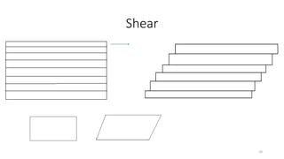
11. Shear
•x’ = x + yshx
•y’ = y
[P'] = [T] [P]
x’
y’
x
y
=
1 Shx
Shy 1
•x’ = x
•y’ = y + xshy
x’
y’
x
y
=
1 Shx
0 1
x’
y’
x
y
=
1 0
Shy 1
11

12. 2D Transformations
12
x’
y’
x
y
tx
ty
= +
x’
y’
x
y
=
cos -sin
sin cos
x’
y’
x
y
=
Sx 0
0 Sy
x’
y’
x
y
= 1 0
0 -1
x’
y’
x
y
=
-1 0
0 1
x’
y’
x
y
=
1 Shx
Shy 1
[P'] = [ T] + [P]
[P'] = [T] [P]

13. Homogeneous Coordinates and Homogeneous
Transformations
• All the transformations, except translation, are in the form of matrix
multiplication.
• “Translation” takes the form of vector addition.
• This makes it inconvenient to concatenate transformations involving
translation.
• It is therefore desirable to express all geometric transformations in the
form of matrix multiplication only.
13

14. Homogeneous Coordinates and Homogeneous
Transformations
• Many graphics applications involve sequence of geometric
transformations.
• Animations also require an object to be translated, rotated, scaled, etc.
at an each increment of a motion sequence.
• In design and picture construction applications different transformations
are used to fit the picture components into their proper positions.
14

15. Homogeneous Coordinates and Homogeneous
Transformations
• Representing points by their homogeneous coordinates, provides an
effective way to unify the description of geometric transformations
as matrix multiplication.
• Homogeneous coordinates have been used in computer graphics and
geometric modelling techniques.
• With the help of homogeneous coordinates, geometric
transformations are customarily embedded into graphics hardware to
speed their execution.
15

16. Homogeneous Coordinates and
Homogeneous Transformations
• In a 2D space, point P with Cartesian coordinates (X, Y), has
homogeneous coordinates (X*, Y* , h), where h is a scalar factor and
h≠0.
• P (X, Y)………………….. Cartesian coordinates
• P(X*, Y* , h)……………….. Homogeneous coordinates
16

17. Homogeneous Coordinates and Homogeneous
Transformations
• Cartesian and Homogeneous coordinates are related to each other by
following relation
𝑋 =
X∗
ℎ
, 𝑌 =
Y∗
ℎ
, Z =
𝑍∗
ℎ
• Above equations are based on the fact that, if the Cartesian coordinates
of a given point P are multiplied by scalar factor h, then P is scaled to a
new point P∗ and the coordinates of P and P∗ are related by above
equations.
17

18. Homogeneous Coordinates and Homogeneous
Transformations
• For the purpose of geometric transformations the scalar factor h is
taken to be Unity to avoid unnecessary divisions.
𝑃 𝑋, 𝑌 = 𝑃(𝑋, 𝑌, 1)
• By using homogeneous coordinates, all the 5 types of
transformations that is, translation, rotation, scaling, mirror (reflect)
and shear, can be represented as a product of “3 X 3” transformation
matrix and “3 x 1” column vector.
18

19. Homogeneous Coordinates and Homogeneous
Transformations
• The conversion of two dimensional co-ordinate pair (x, y), into a three
dimensional vector (x, y ,1), is known as Homogeneous
representation.
19

20. x’
y’
x
y
tx
ty
= +
x’
y’
x
y
=
cos -sin
sin cos
x’
y’
1
1 0 tx
0 1 ty
0 0 1
=
x
Y
1
x’
y’
1
cos -sin 0
sin cos 0
0 0 1
=
x
Y
1
Homogeneous Coordinates and Homogeneous
Transformations
20
1. Translation
2. Rotation
3*3 3*1
3*1

21. x’
y’
x
y
=
Sx 0
0 Sy
x’
y’
x
y
= 1 0
0 -1
x’
y’
x
y
=
-1 0
0 1
x’
y’
1
Sx 0 0
0 Sy 0
0 0 1
=
x
Y
1
x’
y’
1
1 0 0
0 -1 0
0 0 1
=
x
Y
1
x’
y’
1
-1 0 0
0 1 0
0 0 1
=
x
Y
1
3. Scaling
4. Mirror/ Reflection
Homogeneous Coordinates and Homogeneous
Transformations
21

22. x’
y’
x
y
=
1 Shx
Shy 1
x’
y’
1
1 Shx 0
Shy 1 0
0 0 1
=
x
Y
1
5. Shear
Homogeneous Coordinates and Homogeneous
Transformations
22

23. x’
y’
1
1 0 tx
0 1 ty
0 0 1
=
x
Y
1
x’
y’
1
cos -sin 0
sin cos 0
0 0 1
=
x
Y
1
x’
y’
1
Sx 0 0
0 Sy 0
0 0 1
=
x
Y
1
x’
y’
1
1 0 0
0 -1 0
0 0 1
=
x
Y
1
x’
y’
1
-1 0 0
0 1 0
0 0 1
=
x
Y
1
x’
y’
1
1 Shx 0
Shy 1 0
0 0 1
=
x
Y
1
Shearing /shear
Translation
Rotation
Scaling
X Mirror / Reflect Y Mirror / Reflect
23

24. Homogeneous Coordinates and Homogeneous
Transformations
• This 3D representation of a 2D space is called as homogeneous
coordinate system and transformation using homogeneous
coordinates are called as homogeneous transformations.
• Expressing positions in homogeneous coordinate system allow the
users to represent geometric transformations in the form of matrix
multiplication.
24

25. Composite Transformations /
Concatenations
25
[P'] = [Tn] [Tn-1] [Tn-2]…… [T3] [T2] [T1] [P]
[P'] = [T] [P]
[T1], [T2], [T3],…….., [Tn-2], [Tn-1],[Tn]

26. 1. Point “A” (4,3) is rotated counterclockwise by 45°. Find the rotation
matrix and coordinates of the resultant point.
26

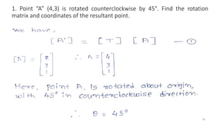
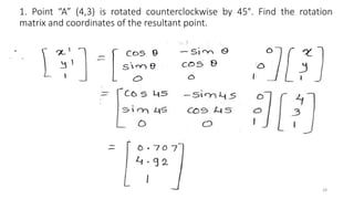
27. 1. Point “A” (4,3) is rotated counterclockwise by 45°. Find the rotation matrix and
coordinates of the resultant point.
27
[A']
[T]Rotation
[A]
[T]

28. 1. Point “A” (4,3) is rotated counterclockwise by 45°. Find the rotation
matrix and coordinates of the resultant point.
28

29. 2. Translate a polygon PQR, P(2,5), Q(7,10) and R(10,2), by 3 units in X
direction and 4 units in Y direction. Identify the transformed coordinates.
29

30. 2. Translate a polygon PQR, P(2,5), Q(7,10) and R(10,2), by 3 units in X
direction and 4 units in Y direction. Identify the transformed coordinates.
30

31. 2. Translate a polygon PQR, P(2,5), Q(7,10) and R(10,2), by 3 units in X
direction and 4 units in Y direction. Identify the transformed coordinates.
31

32. 2. Translate a polygon PQR, P(2,5), Q(7,10) and R(10,2), by 3 units in X
direction and 4 units in Y direction. Identify the transformed coordinates.
32

33. 2. Translate a polygon PQR, P(2,5), Q(7,10) and R(10,2), by 3 units in X
direction and 4 units in Y direction. Identify the transformed coordinates.
33

34. 2. Translate a polygon PQR, P(2,5), Q(7,10) and R(10,2), by 3 units in X
direction and 4 units in Y direction. Identify the transformed coordinates.
34

35. 3. Polygon ABC, A (2,3), B( 0,10) and C(5,10), is moved in such a way that, new
coordinates of point A are (10,10). Find transformation matrix and the resultant
coordinates.
35

36. 3. Polygon ABC, A (2,3), B( 0,10) and C(5,10), is moved in such a way that, new
coordinates of point A are (10,10). Find transformation matrix and the resultant
coordinates.
36

37. 3. Polygon ABC, A (2,3), B( 0,10) and C(5,10), is moved in such a way that, new
coordinates of point A are (10,10). Find transformation matrix and the resultant
coordinates.
37

38. Thank You