This section expands on frequency distributions by discussing additional features: midpoints, which are the averages of class limits; relative frequency, which shows what portion of the data falls in each class; and cumulative frequency, which is the running total of all previous classes' frequencies. It provides an example calculating these values for a given

1. Chapter 2 Descriptive Statistics Larson/Farber 4th ed.

2. Section 2.1 Frequency Distributions and Their Graphs Part 1: Frequency Distributions Larson/Farber 4th ed.

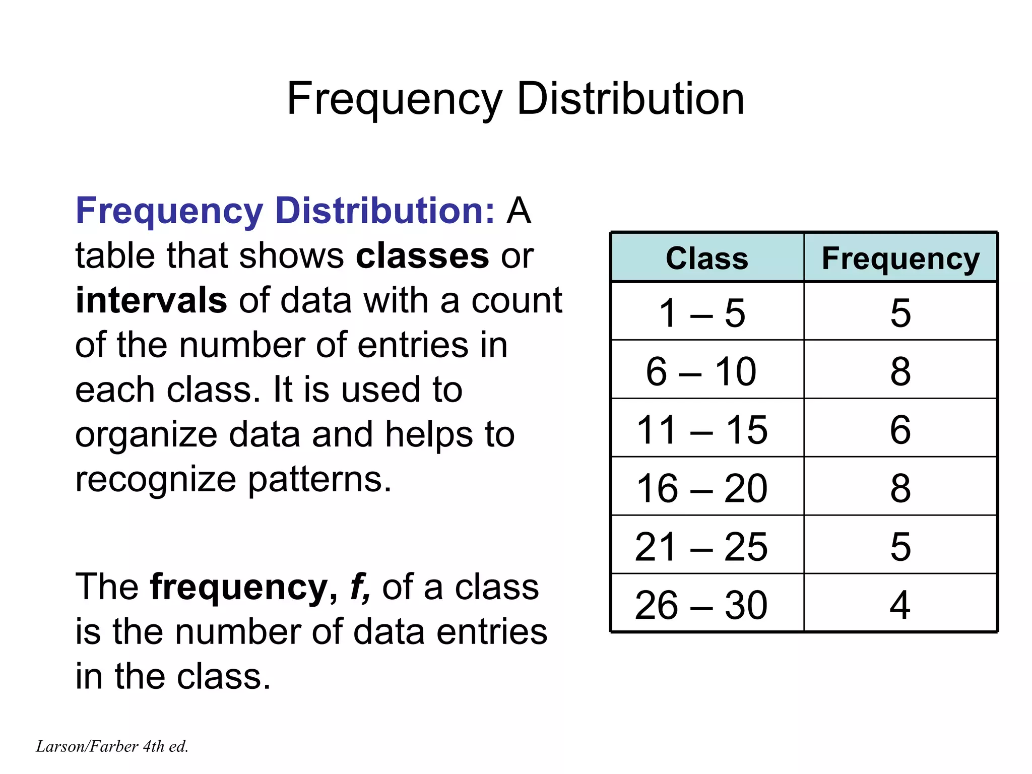
3. Frequency Distribution Frequency Distribution: A table that shows classes or intervals of data with a count of the number of entries in each class. It is used to organize data and helps to recognize patterns. The frequency, f, of a class is the number of data entries in the class. Larson/Farber 4th ed. 4 26 – 30 5 21 – 25 8 16 – 20 6 11 – 15 8 6 – 10 5 1 – 5 Frequency Class

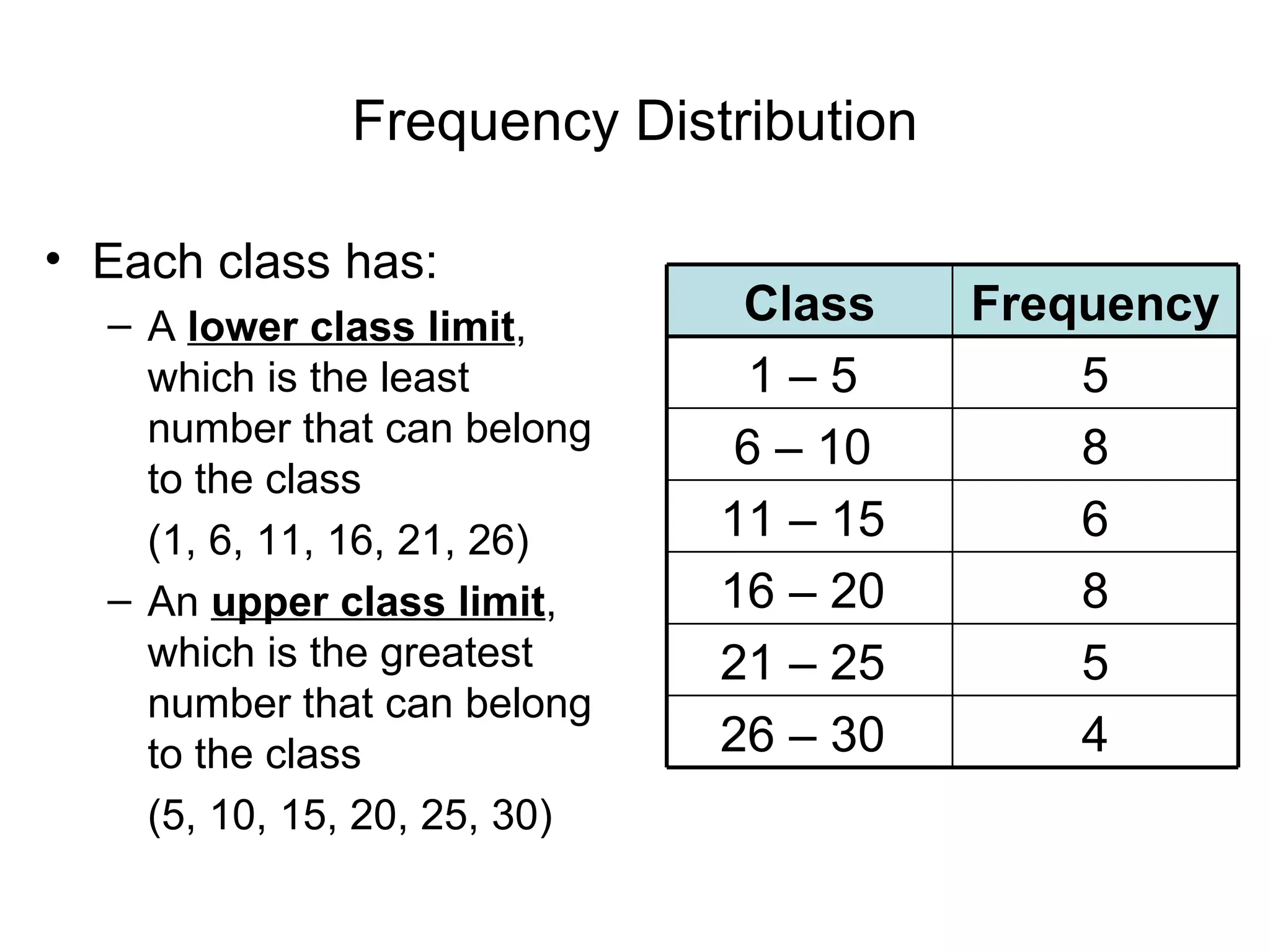
4. Frequency Distribution Each class has: A lower class limit , which is the least number that can belong to the class (1, 6, 11, 16, 21, 26) An upper class limit , which is the greatest number that can belong to the class (5, 10, 15, 20, 25, 30) 4 26 – 30 5 21 – 25 8 16 – 20 6 11 – 15 8 6 – 10 5 1 – 5 Frequency Class

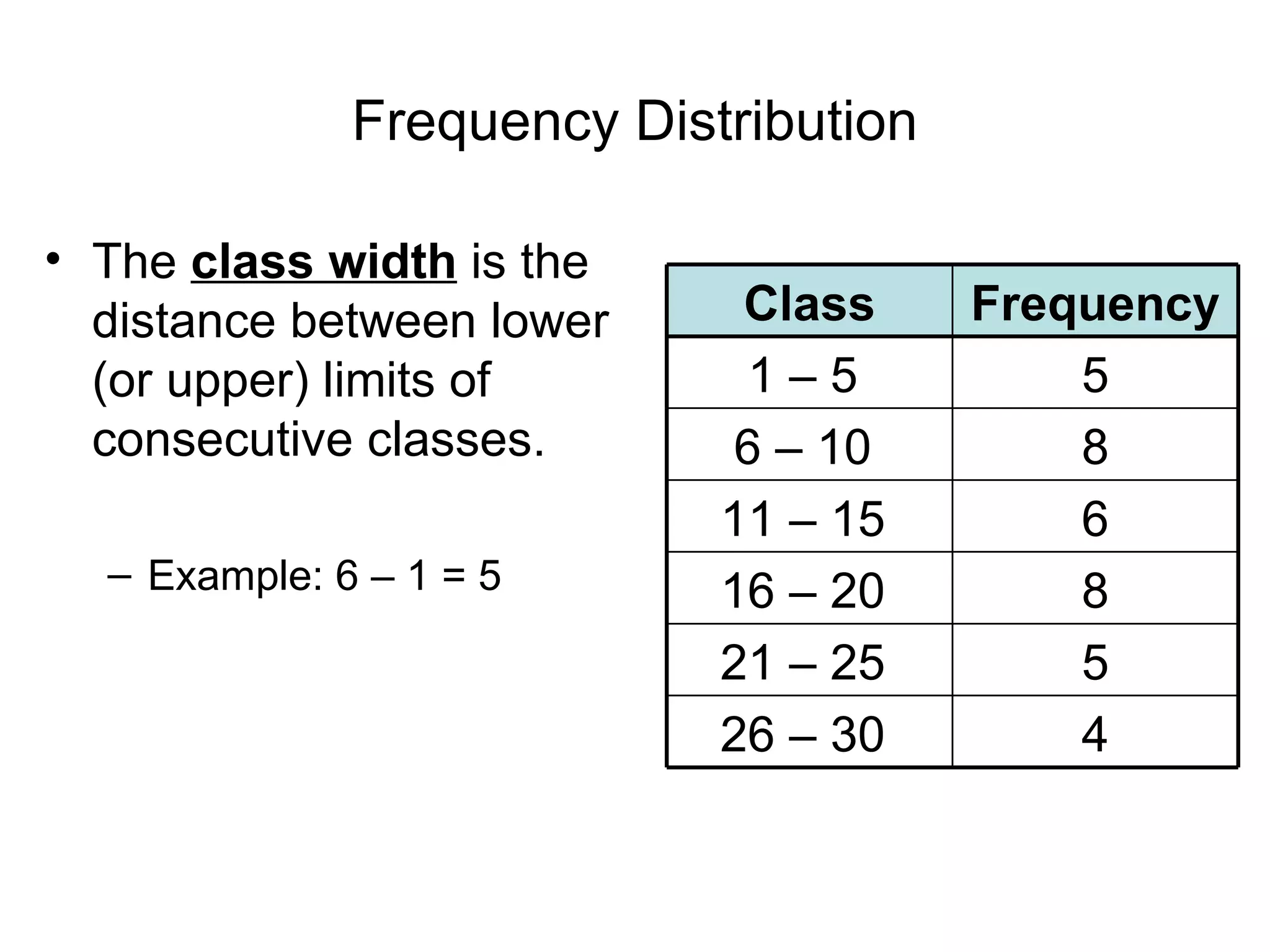
5. Frequency Distribution The class width is the distance between lower (or upper) limits of consecutive classes. Example: 6 – 1 = 5 4 26 – 30 5 21 – 25 8 16 – 20 6 11 – 15 8 6 – 10 5 1 – 5 Frequency Class

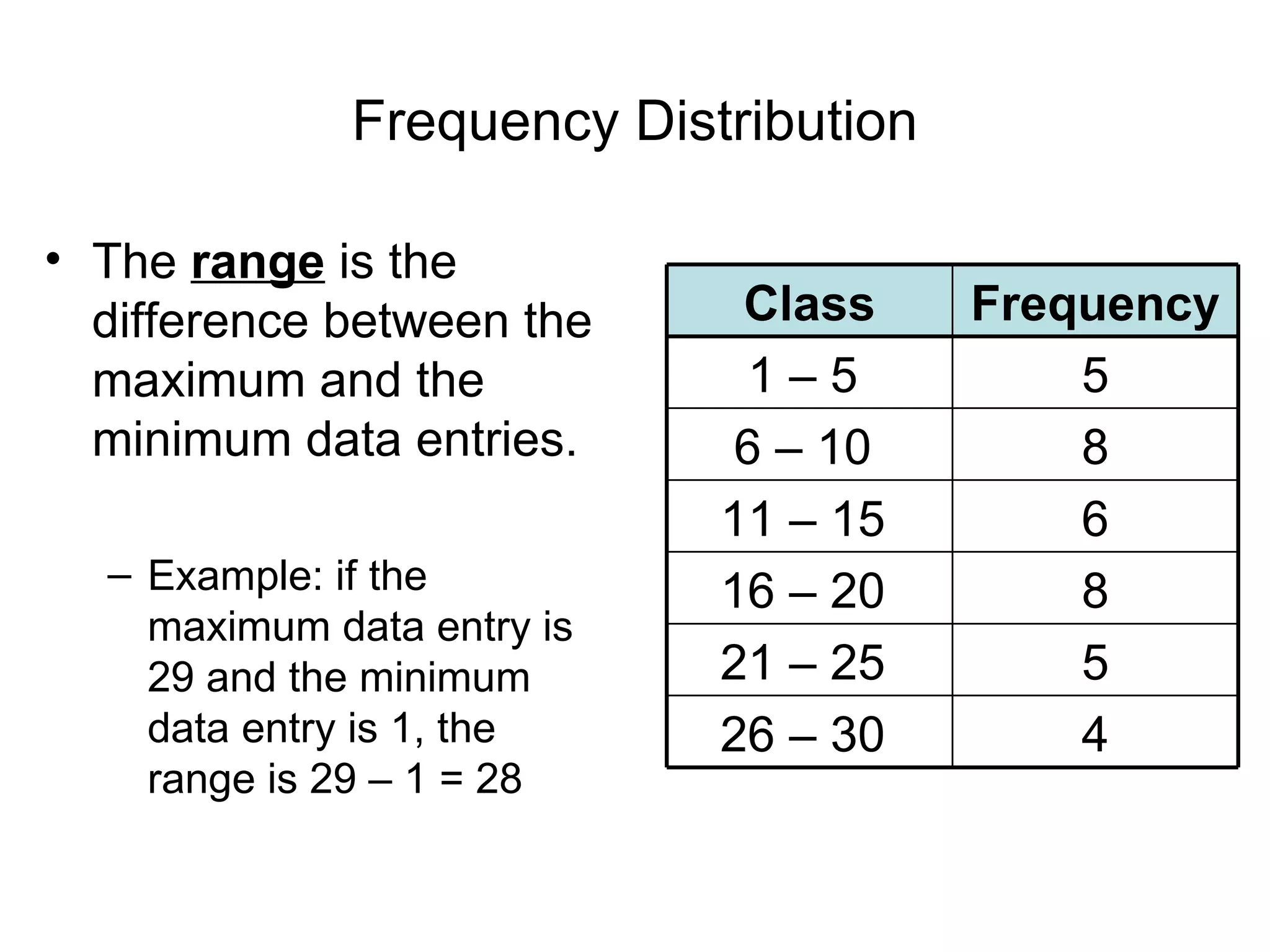
6. Frequency Distribution The range is the difference between the maximum and the minimum data entries. Example: if the maximum data entry is 29 and the minimum data entry is 1, the range is 29 – 1 = 28 4 26 – 30 5 21 – 25 8 16 – 20 6 11 – 15 8 6 – 10 5 1 – 5 Frequency Class

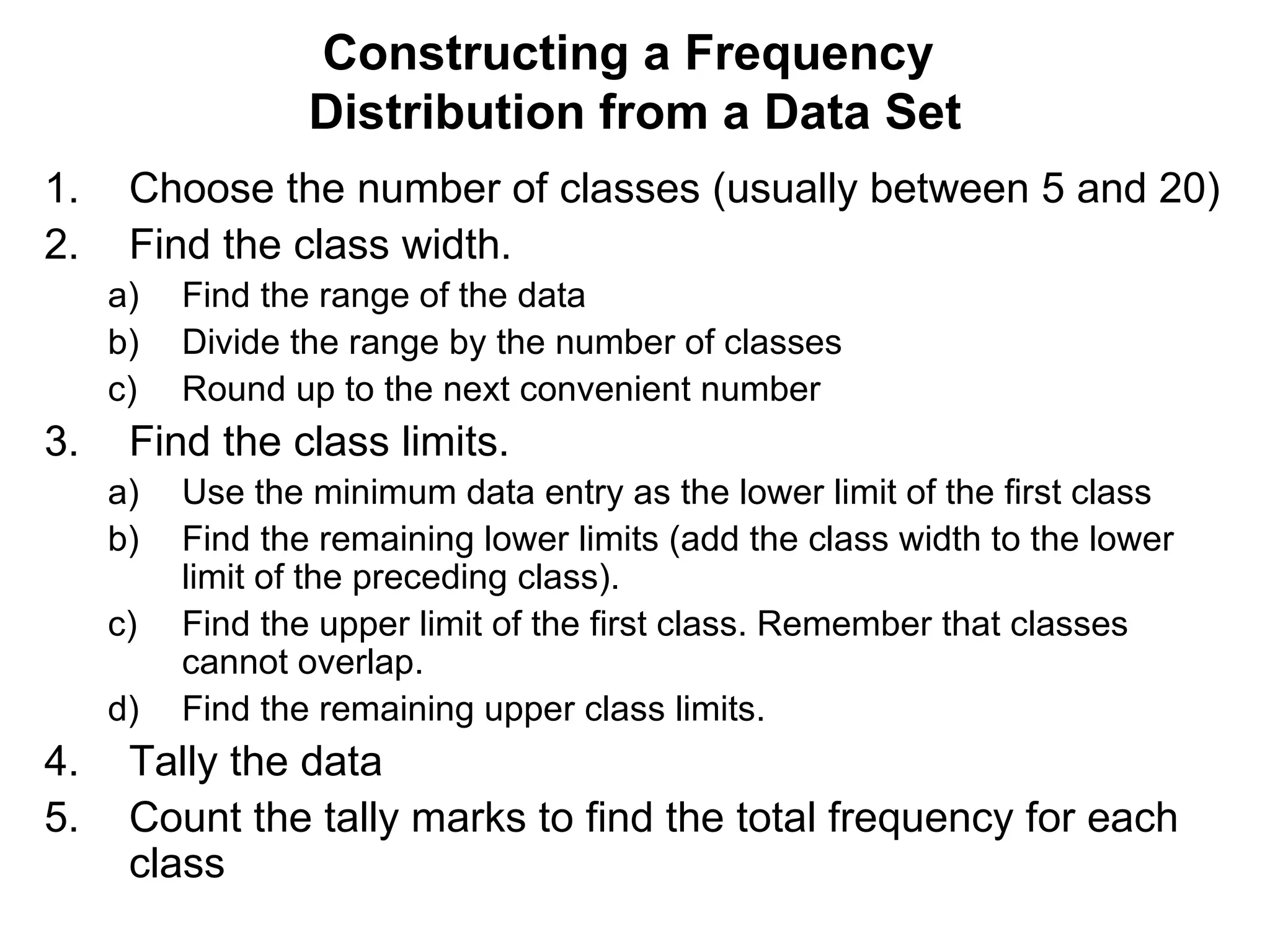
7. Constructing a Frequency Distribution from a Data Set Choose the number of classes (usually between 5 and 20) Find the class width. Find the range of the data Divide the range by the number of classes Round up to the next convenient number Find the class limits. Use the minimum data entry as the lower limit of the first class Find the remaining lower limits (add the class width to the lower limit of the preceding class). Find the upper limit of the first class. Remember that classes cannot overlap. Find the remaining upper class limits. Tally the data Count the tally marks to find the total frequency for each class

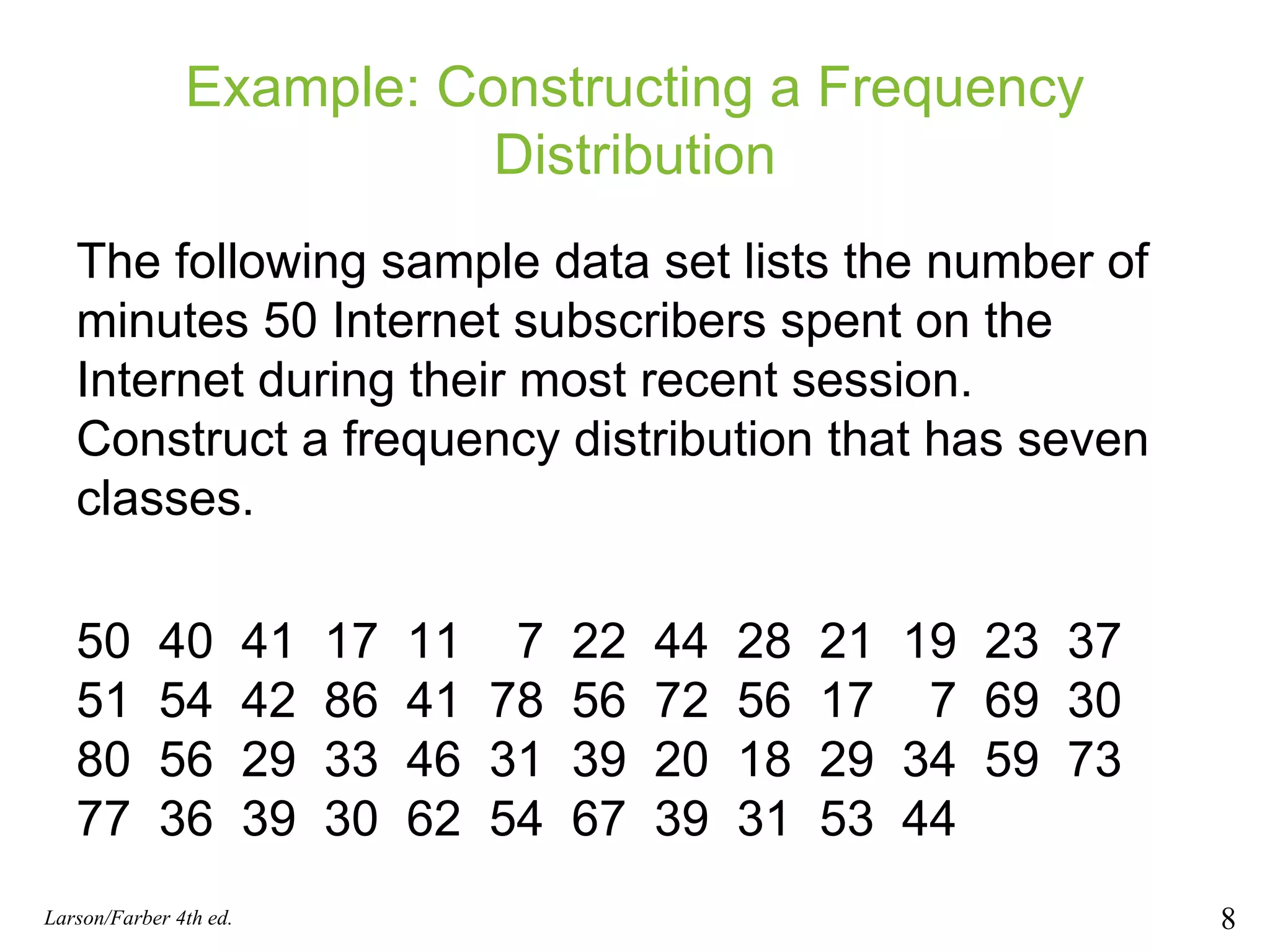
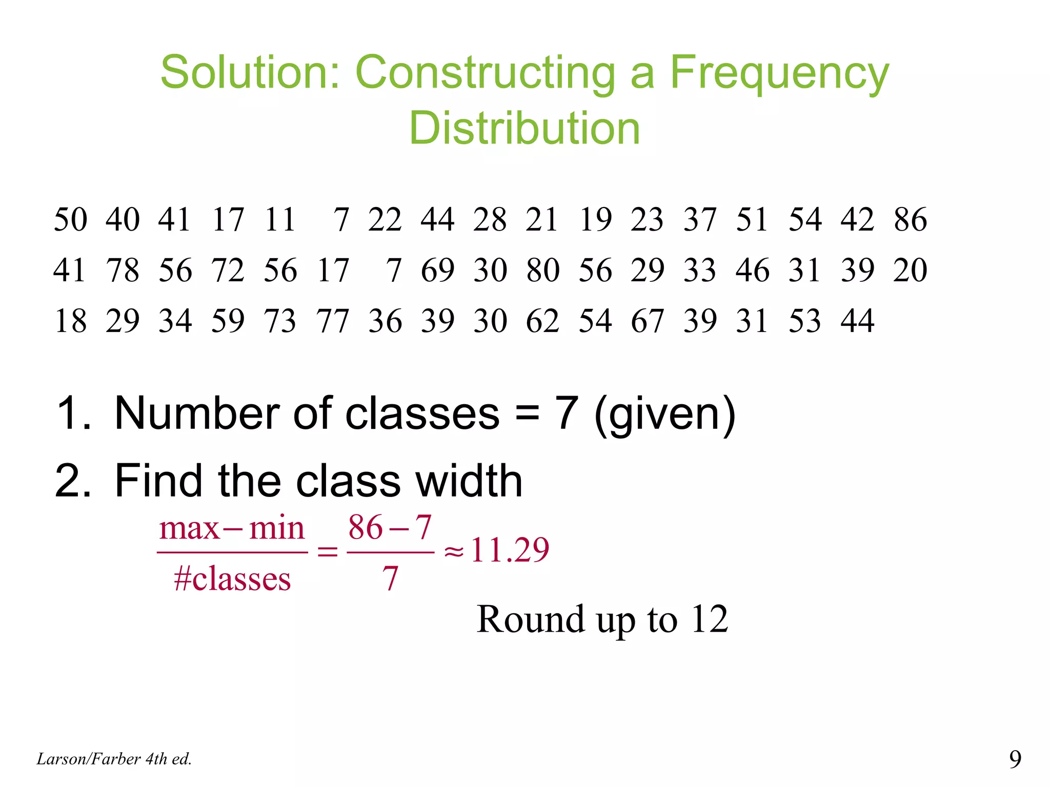
8. Example: Constructing a Frequency Distribution The following sample data set lists the number of minutes 50 Internet subscribers spent on the Internet during their most recent session. Construct a frequency distribution that has seven classes. 50 40 41 17 11 7 22 44 28 21 19 23 37 51 54 42 86 41 78 56 72 56 17 7 69 30 80 56 29 33 46 31 39 20 18 29 34 59 73 77 36 39 30 62 54 67 39 31 53 44 Larson/Farber 4th ed.

9. Solution: Constructing a Frequency Distribution Number of classes = 7 (given) Find the class width Larson/Farber 4th ed. Round up to 12 50 40 41 17 11 7 22 44 28 21 19 23 37 51 54 42 86 41 78 56 72 56 17 7 69 30 80 56 29 33 46 31 39 20 18 29 34 59 73 77 36 39 30 62 54 67 39 31 53 44

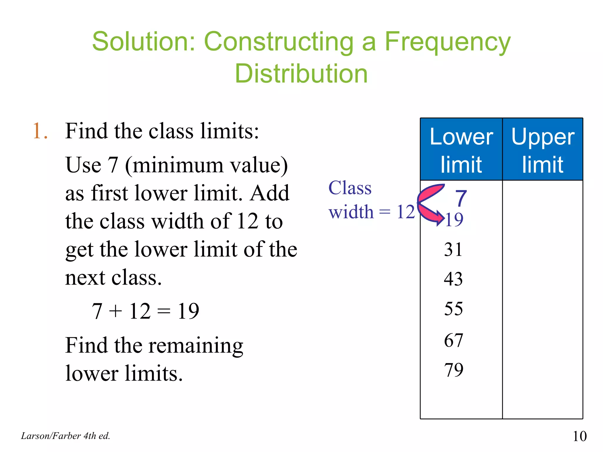
10. Solution: Constructing a Frequency Distribution Larson/Farber 4th ed. Class width = 12 Find the class limits: Use 7 (minimum value) as first lower limit. Add the class width of 12 to get the lower limit of the next class. 7 + 12 = 19 Find the remaining lower limits. 19 31 43 55 67 79 Lower limit Upper limit 7

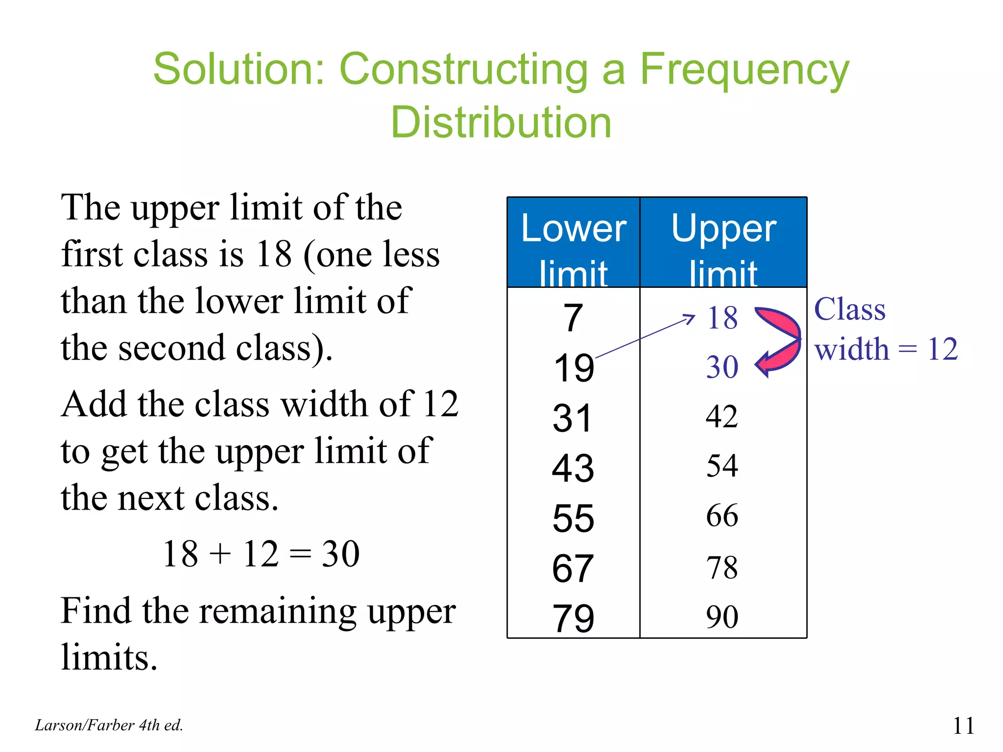
11. Solution: Constructing a Frequency Distribution The upper limit of the first class is 18 (one less than the lower limit of the second class). Add the class width of 12 to get the upper limit of the next class. 18 + 12 = 30 Find the remaining upper limits. Larson/Farber 4th ed. Class width = 12 30 42 54 66 78 90 18 Lower limit Upper limit 7 19 31 43 55 67 79

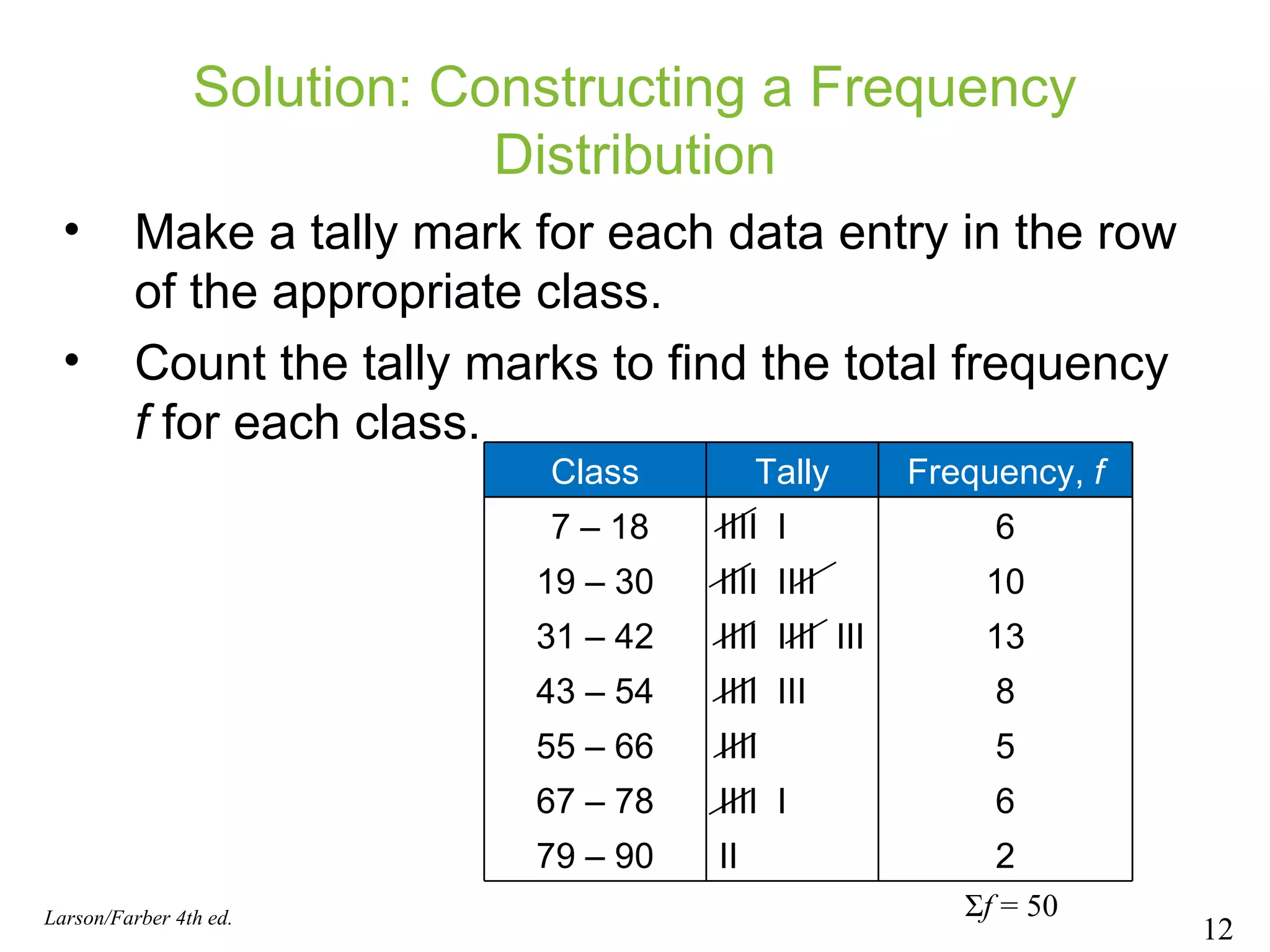
12. Solution: Constructing a Frequency Distribution Make a tally mark for each data entry in the row of the appropriate class. Count the tally marks to find the total frequency f for each class. Larson/Farber 4th ed. Σ f = 50 Class Tally Frequency, f 7 – 18 IIII I 6 19 – 30 IIII IIII 10 31 – 42 IIII IIII III 13 43 – 54 IIII III 8 55 – 66 IIII 5 67 – 78 IIII I 6 79 – 90 II 2

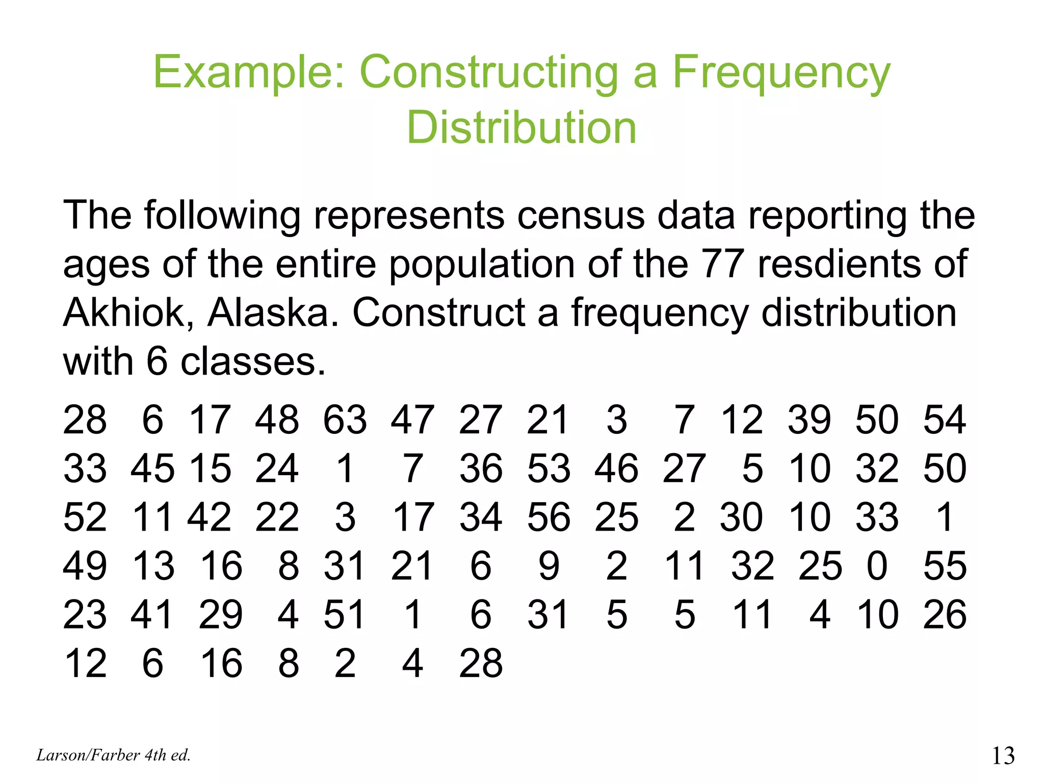
13. Example: Constructing a Frequency Distribution The following represents census data reporting the ages of the entire population of the 77 resdients of Akhiok, Alaska. Construct a frequency distribution with 6 classes. 28 6 17 48 63 47 27 21 3 7 12 39 50 54 33 45 15 24 1 7 36 53 46 27 5 10 32 50 52 11 42 22 3 17 34 56 25 2 30 10 33 1 49 13 16 8 31 21 6 9 2 11 32 25 0 55 23 41 29 4 51 1 6 31 5 5 11 4 10 26 12 6 16 8 2 4 28 Larson/Farber 4th ed.

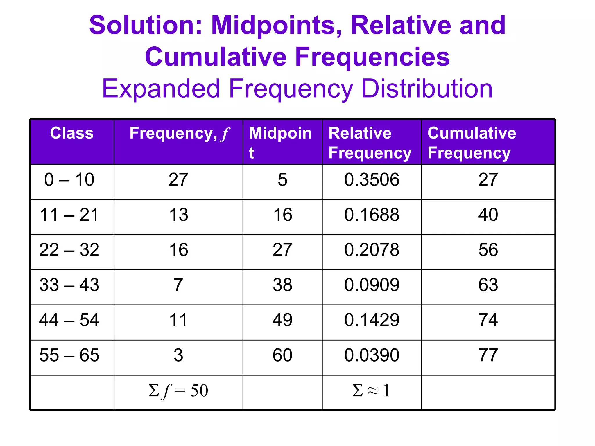
14. Expanding the Frequency Distribution There are additional features that we can add to the frequency distribution that will provide a better understanding of the data Midpoint, relative frequency, and cumulative frequency

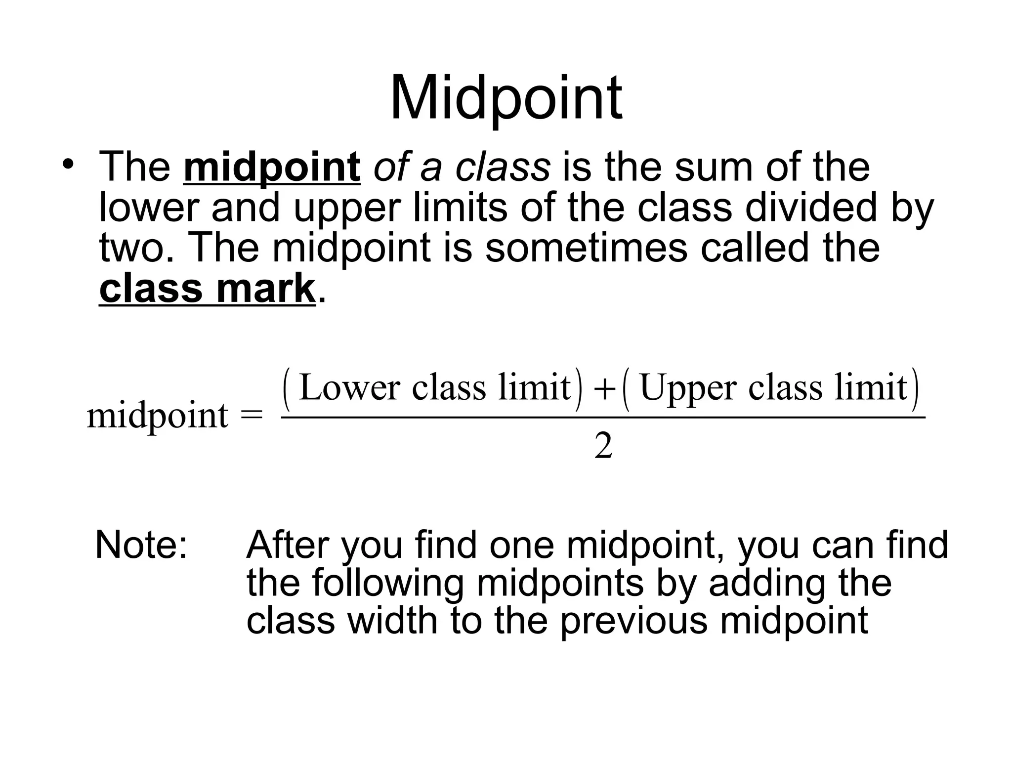
15. Midpoint The midpoint of a class is the sum of the lower and upper limits of the class divided by two. The midpoint is sometimes called the class mark . Note: After you find one midpoint, you can find the following midpoints by adding the class width to the previous midpoint

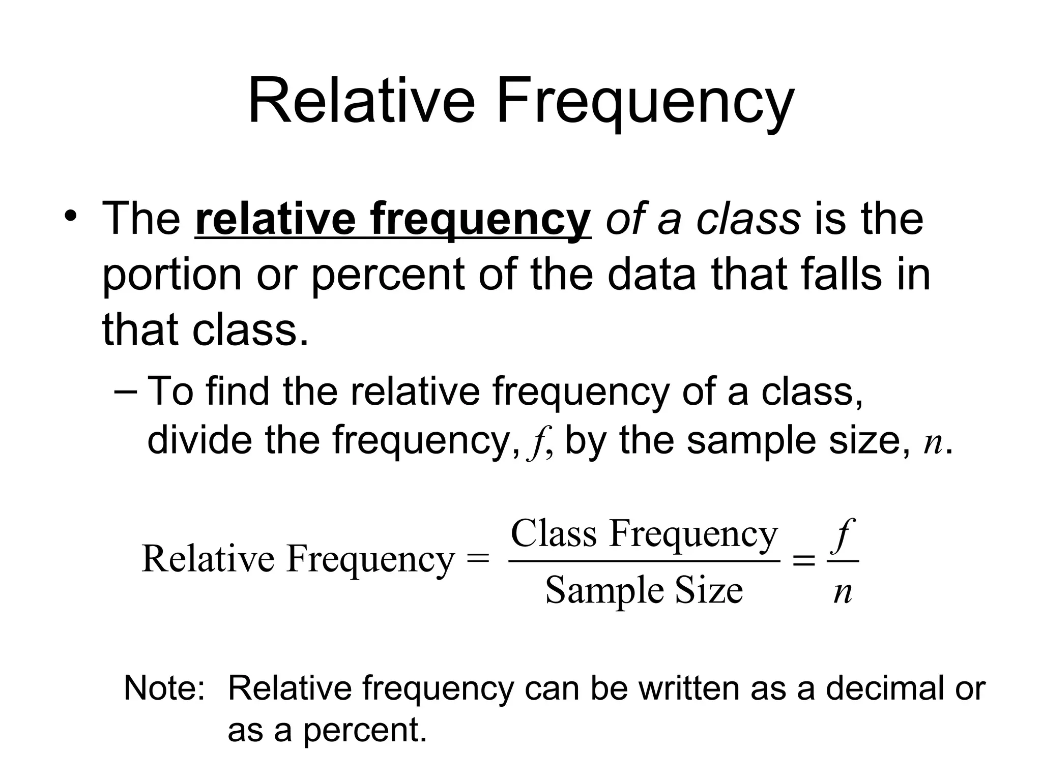
16. Relative Frequency The relative frequency of a class is the portion or percent of the data that falls in that class. To find the relative frequency of a class, divide the frequency, f , by the sample size, n . Note: Relative frequency can be written as a decimal or as a percent.

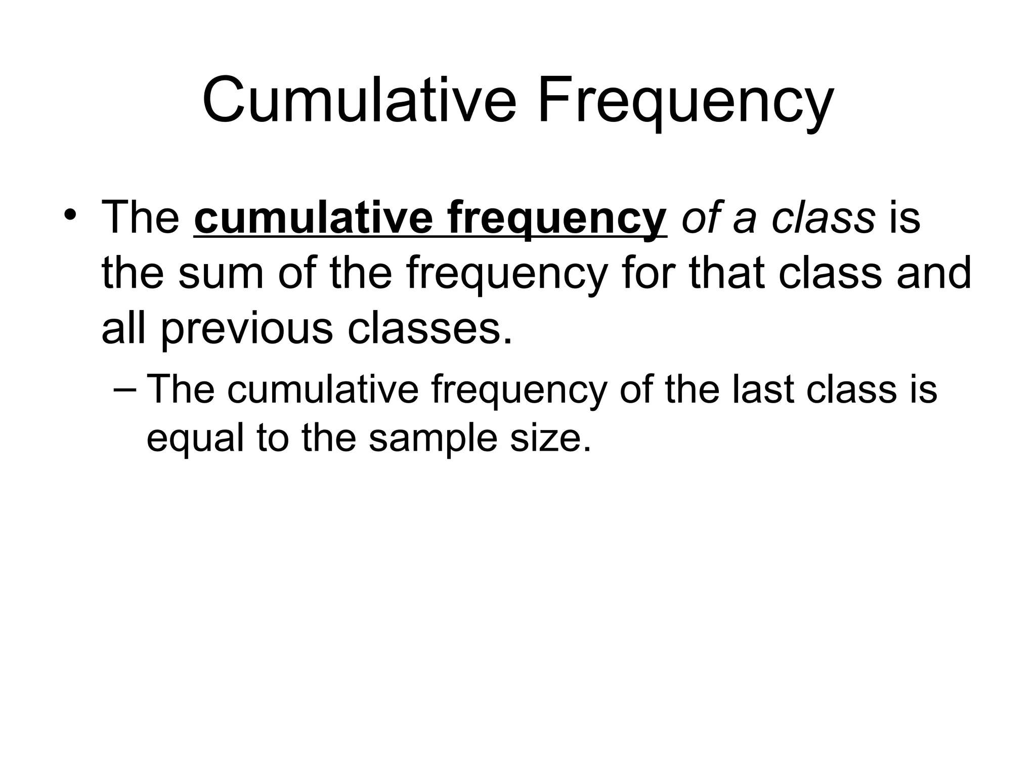
17. Cumulative Frequency The cumulative frequency of a class is the sum of the frequency for that class and all previous classes. The cumulative frequency of the last class is equal to the sample size.

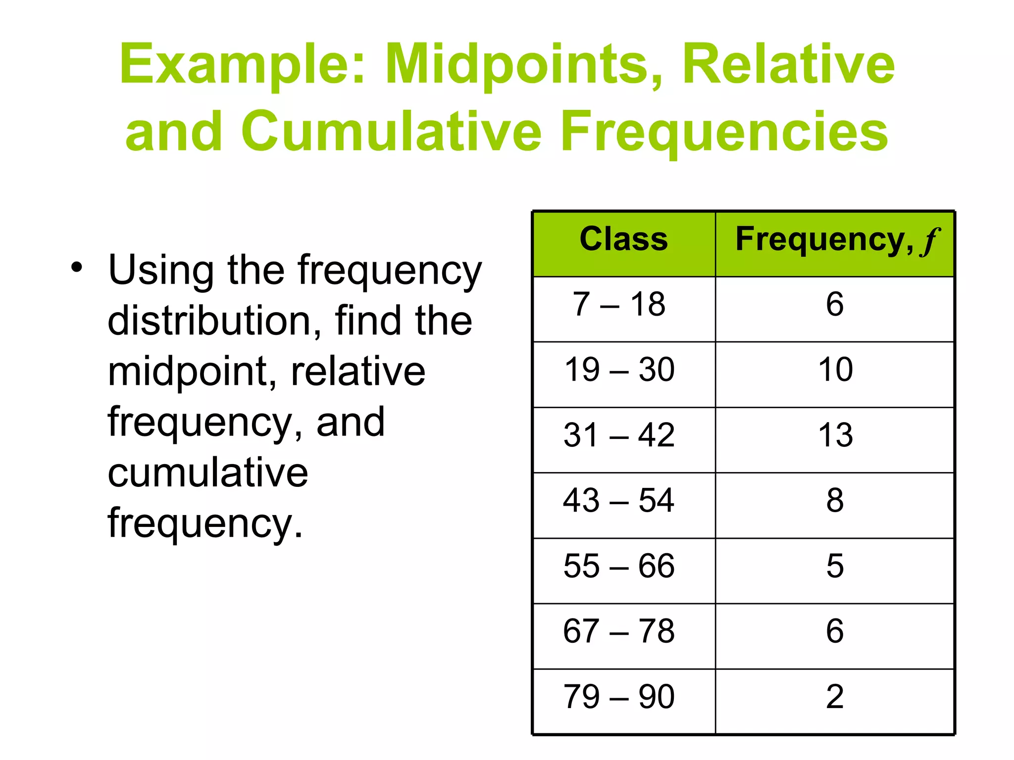
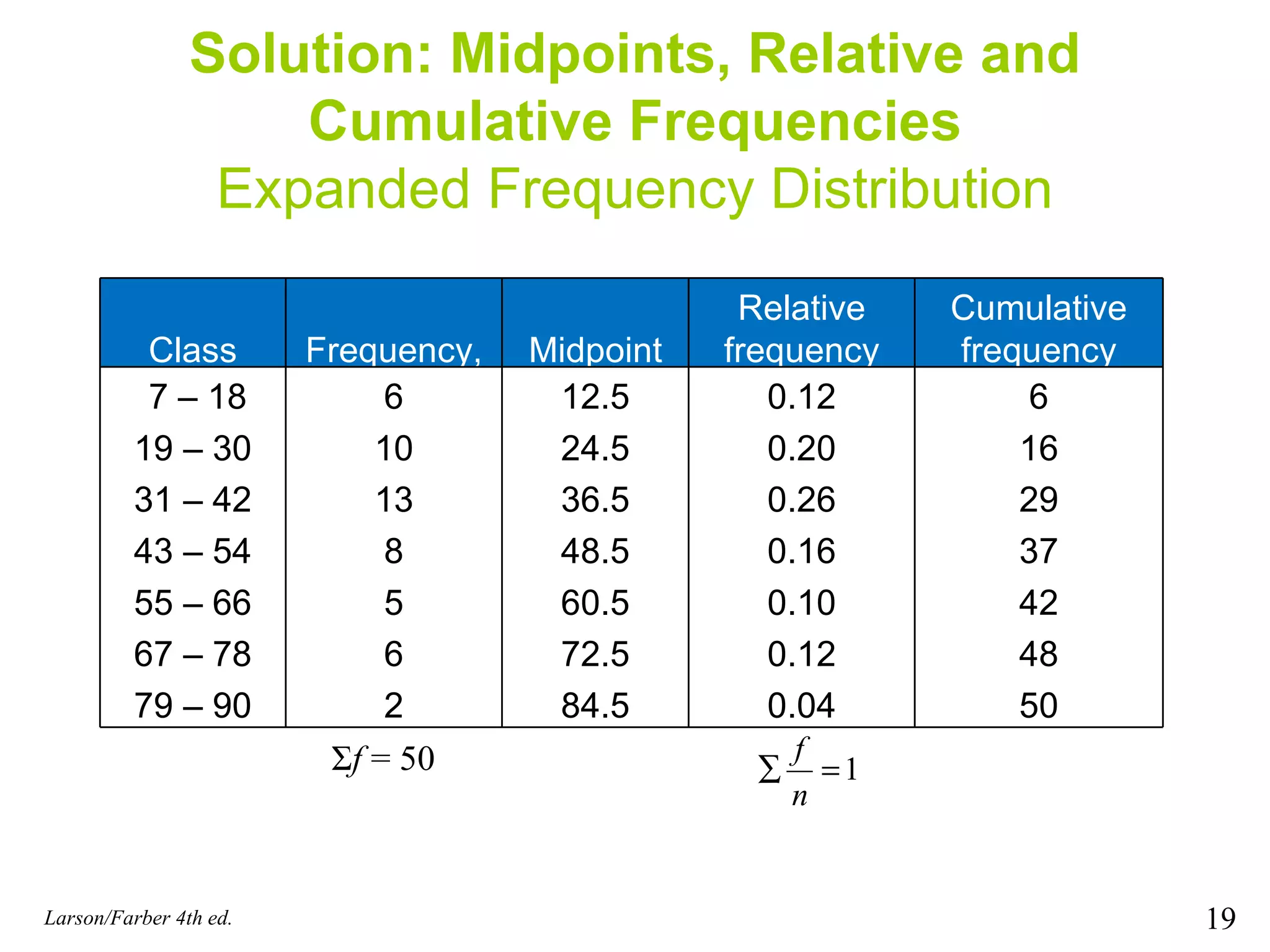
18. Example: Midpoints, Relative and Cumulative Frequencies Using the frequency distribution, find the midpoint, relative frequency, and cumulative frequency. 2 79 – 90 6 67 – 78 5 55 – 66 8 43 – 54 13 31 – 42 10 19 – 30 6 7 – 18 Frequency, f Class

19. Solution: Midpoints, Relative and Cumulative Frequencies Expanded Frequency Distribution Larson/Farber 4th ed. Σ f = 50 Class Frequency, f Midpoint Relative frequency Cumulative frequency 7 – 18 6 12.5 0.12 6 19 – 30 10 24.5 0.20 16 31 – 42 13 36.5 0.26 29 43 – 54 8 48.5 0.16 37 55 – 66 5 60.5 0.10 42 67 – 78 6 72.5 0.12 48 79 – 90 2 84.5 0.04 50

20. Example: Midpoints, Relative and Cumulative Frequencies Using the frequency distribution, find the midpoint, relative frequency, and cumulative frequency. 3 55 – 65 11 44 – 54 7 33 – 43 16 22 – 32 13 11 – 21 5 0 – 10 Frequency, f Class

21. Solution: Midpoints, Relative and Cumulative Frequencies Expanded Frequency Distribution 55 – 65 44 – 54 33 – 43 22 – 32 11 – 21 0 – 10 Class Σ f = 50 3 11 7 16 13 27 Frequency, f Σ ≈ 1 77 0.0390 60 74 0.1429 49 63 0.0909 38 56 0.2078 27 40 0.1688 16 27 0.3506 5 Cumulative Frequency Relative Frequency Midpoint

22. Homework P41 #1, 3 – 6, 15, 16