1. Manifest knowledgeand skills on the principles
and concepts of frequency distribution.
2. Solve problems involving frequency distribution.
3.
Data may bearranged alphabetically, chronologically,
in rank form or by using arrays. The choice of arrangement
depends on the purpose of the researcher. Data are
classified into group and ungroup. The former is the
number of things considered together or regarded as
belonging together while the latter is disarray data.
Introduction
4.
For ungrouped datadistribution, a researcher
may adopt the usual method of listing the respondents
in alphabetical manner. However, the scores are difficult
to interpret. A more convenient way to interpret the data
is using the array method - arranging the scores in
descending or ascending order of magnitude
Ungrouped and Grouped Data
5.
For grouped datadistribution, an array may help
make the overall pattern of data apparent. However, if
the number of scores is large, construction of the array
may have to be done on a computer. Thus, if the
researcher wanted to present the data can adopt a
frequency distribution - tabular presentation that
shows number of data items that fall in each of several
distinct classes.
Ungrouped and Grouped Data
6.
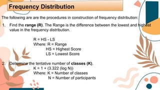
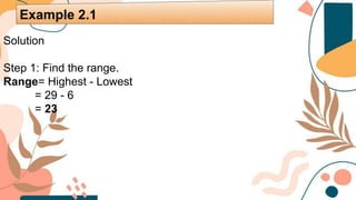
The following arethe procedures in construction of frequency distribution:
1. Find the range (R). The Range is the difference between the lowest and highest
value in the frequency distribution.The mathematical expression for the range is
shown below.
R = HS - LS
Where: R = Range
HS = Highest Score
LS = Lowest Score
Frequency Distribution
7.
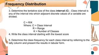
The following areare the procedures in construction of frequency distribution:
1. Find the range (R). The Range is the difference between the lowest and highest
value in the frequency distribution.
R = HS - LS
Where: R = Range
HS = Highest Score
LS = Lowest Score
2. Determine the tentative number of classes (K).
K = 1 + (3.322 (log N))
Where: K = Number of classes
N = Number of participants
Frequency Distribution
8.
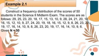
3. Determine thetentative size of the class interval (C) . Class interval is
any of the interval into which adjacent discrete values of a variable are
divided.
C = R/K
Where: C = Class Interval
R = Range
K = Number of Classes
4. Write the class interval starting with the lowest score
5. Determine the class frequency for each class interval by referring to the
tally column and present the results in tabular form.
Frequency Distribution
9.
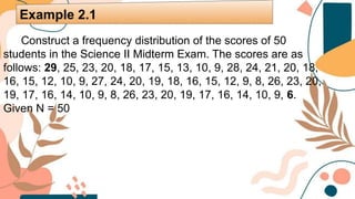
Construct a frequencydistribution of the scores of 50
students in the Science II Midterm Exam. The scores are as
follows: 29, 25, 23, 20, 18, 17, 15, 13, 10, 9, 28, 24, 21, 20, 18,
16, 15, 12, 10, 9, 27, 24, 20, 19, 18, 16, 15, 12, 9, 8, 26, 23, 20,
19, 17, 16, 14, 10, 9, 8, 26, 23, 20, 19, 17, 16, 14, 10, 9, 6.
Given N = 50
Example 2.1
10.
Construct a frequencydistribution of the scores of 50
students in the Science II Midterm Exam. The scores are as
follows: 29, 25, 23, 20, 18, 17, 15, 13, 10, 9, 28, 24, 21, 20, 18,
16, 15, 12, 10, 9, 27, 24, 20, 19, 18, 16, 15, 12, 9, 8, 26, 23, 20,
19, 17, 16, 14, 10, 9, 8, 26, 23, 20, 19, 17, 16, 14, 10, 9, 6.
Given N = 50
Example 2.1
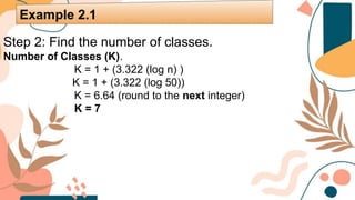
Step 2: Findthe number of classes.
Number of Classes (K).
K = 1 + (3.322 (log n) )
K = 1 + (3.322 (log 50))
K = 6.64 (round to the next integer)
K = 7
Example 2.1
14.
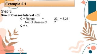
Step 3:
Size ofClasses Interval (C).
C = Range = 23 = 3.28
No. of classes C 7
C = 4
Example 2.1
15.
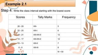
Step 4: Writethe class interval starting with the lowest score
Example 2.1
Scores Tally Marks Frequency
26 - 29 IIIII- 5
22 - 25 IIIII-I 6
18 - 21 IIIII-IIIII-II 12
14 - 17 IIIII-IIIII-II 12
10 - 13 IIIII-II 7
6 - 9 IIIII-III 8
N = 50
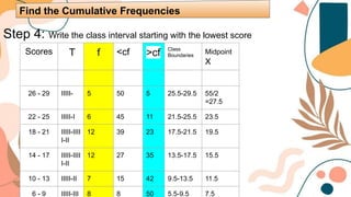
16.
Step 4: Writethe class interval starting with the lowest score
Find the Cumulative Frequencies
Scores T f <cf >cf Class
Boundaries
Midpoint
X
26 - 29 IIIII- 5 50 5 25.5-29.5 55/2
=27.5
22 - 25 IIIII-I 6 45 11 21.5-25.5 23.5
18 - 21 IIIII-IIII
I-II
12 39 23 17.5-21.5 19.5
14 - 17 IIIII-IIII
I-II
12 27 35 13.5-17.5 15.5
10 - 13 IIIII-II 7 15 42 9.5-13.5 11.5
6 - 9 IIIII-III 8 8 50 5.5-9.5 7.5
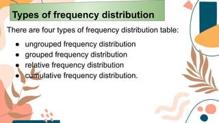
There are fourtypes of frequency distribution table:
● ungrouped frequency distribution
● grouped frequency distribution
● relative frequency distribution
● cumulative frequency distribution.
Types of frequency distribution
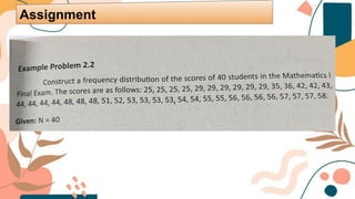
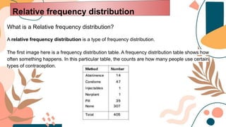
19.
What is aRelative frequency distribution?
A relative frequency distribution is a type of frequency distribution.
The first image here is a frequency distribution table. A frequency distribution table shows how
often something happens. In this particular table, the counts are how many people use certain
types of contraception.
Relative frequency distribution
20.
With a relativefrequency distribution, we don’t want to know the
counts. We want to know the percentages. In other words, what
percentage of people used a particular form of contraception?
Relative frequency distribution
21.
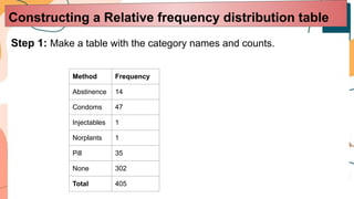
Step 1: Makea table with the category names and counts.
Constructing a Relative frequency distribution table
Method Frequency
Abstinence 14
Condoms 47
Injectables 1
Norplants 1
Pill 35
None 302
Total 405
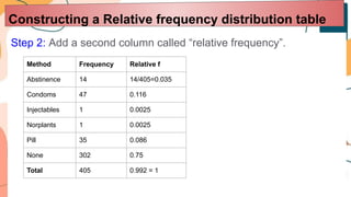
22.
Step 2: Adda second column called “relative frequency”.
Constructing a Relative frequency distribution table
Method Frequency Relative f
Abstinence 14 14/405=0.035
Condoms 47 0.116
Injectables 1 0.0025
Norplants 1 0.0025
Pill 35 0.086
None 302 0.75
Total 405 0.992 = 1
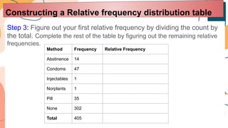
23.
Step 3: Figureout your first relative frequency by dividing the count by
the total. Complete the rest of the table by figuring out the remaining relative
frequencies.
Constructing a Relative frequency distribution table
Method Frequency Relative Frequency
Abstinence 14
Condoms 47
Injectables 1
Norplants 1
Pill 35
None 302
Total 405
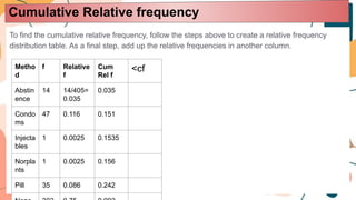
24.
To find thecumulative relative frequency, follow the steps above to create a relative frequency
distribution table. As a final step, add up the relative frequencies in another column.
Cumulative Relative frequency
Metho
d
f Relative
f
Cum
Rel f
<cf
Abstin
ence
14 14/405=
0.035
0.035
Condo
ms
47 0.116 0.151
Injecta
bles
1 0.0025 0.1535
Norpla
nts
1 0.0025 0.156
Pill 35 0.086 0.242
25.
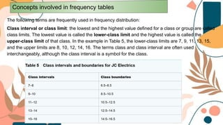
The following termsare frequently used in frequency distribution:
Class interval or class limit: the lowest and the highest value defined for a class or group are called
class limits. The lowest value is called the lower-class limit and the highest value is called the
upper-class limit of that class. In the example in Table 5, the lower-class limits are 7, 9, 11, 13, 15,
and the upper limits are 8, 10, 12, 14, 16. The terms class and class interval are often used
interchangeably, although the class interval is a symbol for the class.
Concepts involved in frequency tables
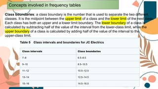
26.
Class boundaries: aclass boundary is the number that is used to separate the two different
classes. It is the midpoint between the upper limit of a class and the lower limit of the next class.
Each class has both an upper and a lower limit boundary. The lower boundary of a class is
calculated by subtracting half of the value of the interval from the lower-class limit, while the
upper boundary of a class is calculated by adding half of the value of the interval to the
upper-class limit.
Concepts involved in frequency tables
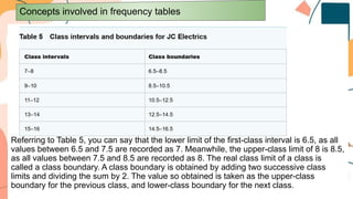
27.
Referring to Table5, you can say that the lower limit of the first-class interval is 6.5, as all
values between 6.5 and 7.5 are recorded as 7. Meanwhile, the upper-class limit of 8 is 8.5,
as all values between 7.5 and 8.5 are recorded as 8. The real class limit of a class is
called a class boundary. A class boundary is obtained by adding two successive class
limits and dividing the sum by 2. The value so obtained is taken as the upper-class
boundary for the previous class, and lower-class boundary for the next class.
Concepts involved in frequency tables
28.
Midpoint or classmark: this is the average of a class interval, and is obtained
by dividing the sum of upper- and lower-class limits by 2. Thus, the class mark of
the interval 7–8 is 7.5, as (7+8)/2=7.5.
The size or the width of a class interval: the size, or width, of a class interval
is the difference between the lower- and upper-class boundaries and is also
referred to as the class width, class size, or class length. If all class intervals of a
frequency distribution have equal widths, this common width is denoted by c.
Range: this is the difference between the maximum value and the minimum
value of the data set. For example, in the JC Electrics data set the maximum
number of Electric Motors sold has a value of 25, while the minimum is 14.
Hence, to calculate the range, you must calculate 25–14=11.
Concepts involved in frequency tables