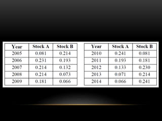
MEAN,
MEDIAN &
MODE (FOR
GROUPED
DATA)
MS. Maria Christita Polinag
MiriamCollege Adult Education
MEAN for Grouped Data:
Class
Interval
Class
Frequenc
y (f)
Class
Mark (x)
fx
𝑥 =
𝑓1 𝑥1 + 𝑓2 𝑥2 + 𝑓3 𝑥3 + ⋯ 𝑓𝑛−1 𝑥 𝑛−1 + 𝑓𝑛 𝑥 𝑛
𝑁
=
𝛴𝑓𝑥
𝑁
EXAMPLE:
Class Interval Class Frequency (f)
10-20 5
21-31 10
32-42 11
43-53 7
54-64 23
65-75 56
76-86 6
87-97 8
98-108 4
Σf = N = ________
The result of the scores in Mathematics test during theTeacher’s
Board Examination
Find the Mean
Score of all the
examinees.
Class
Interval
Class
Frequency
(f)
Class Mark
(x)
fx
10-20 5 15 75
21-31 10 26 260
32-42 11 37 407
43-53 7 48 336
54-64 23 59 1357
65-75 56 70 3920
76-86 6 81 486
87-97 8 92 736
98-108 4 103 412
Σf = N = 130 Σfx = 7989
The result of the scores in Mathematics test during the
Teacher’s Board Examination
𝑥 =
𝛴𝑓𝑥
𝑁
=
7989
130
𝑥 = 61.45
MEDIAN for grouped Data:
Class
Interval
Class
Frequency (f)
< Cumulative
Frequency
(<CF)
𝑀 =
𝑁
2
Median Class is the class
interval to which M is included
with respect to the less than
cumulative frequency.
𝑥 = 𝑥 𝐿𝐵 + 𝑖
𝑁
2
− < 𝑐𝑓𝑏
𝑓𝑚
EXAMPLE:
Class
Interval
Class
Frequency
(f)
< Cumulative
Frequency
(<CF)
10-20 5 5
21-31 10 15
32-42 11 26
43-53 7 33
54-64 23 56
65-75 55 111
76-86 7 118
87-97 8 126
98-108 4 130
Σf =N = 130
Find the Median
class.
𝑀 =
𝑁
2
=
130
2
𝑀 = 65
Class
Interval
Class
Frequency (f)
< Cumulative
Frequency
(<CF)
43-53 7 33
54-64 23 56
65-75 55 111
76-86 7 118
Find the Median for the grouped data
𝑥 = 𝑥 𝐿𝐵 + 𝑖
𝑁
2
− < 𝑐𝑓𝑏
𝑓𝑚
1. Lower class boundary of M
𝑥 𝐿𝐵 = 𝐿𝐿 − 0.5
𝑥 𝐿𝐵= 65 − 0.5
= 64.5
2. Class size (i)
𝑖 = 𝑈𝐿 − 𝐿𝐿 + 1
𝑖 = 75 − 65 + 1
= 11
Class
Interval
Class
Frequency (f)
< Cumulative
Frequency
(<CF)
43-53 7 33
54-64 23 56
65-75 55 111
76-86 7 118
Find the Median for the grouped data
𝑥 = 𝑥 𝐿𝐵 + 𝑖
𝑁
2
− < 𝑐𝑓𝑏
𝑓𝑚
= 64.5 + 11
130
2
− 56
55
𝑥 = 64.5 + 11
65 − 56
55
= 64.5 + 11
9
55
= 64.5 + 11 0.16363
𝑥 = 64.5 + 1.8 = 66.3
3. Less than cumulative
frequency before the median
class
< 𝑐𝑓𝑏 = 56
4. Median class frequency
𝑓𝑚 = 55
MODE for grouped Data:
Class Interval
Class Frequency
(f)
Modal Class is the class interval with the heights class
frequency.
𝑥 = 𝑥 𝐿𝐵 + 𝑖
𝑓𝑚 − 𝑓𝑚𝑏
2𝑓𝑚 − 𝑓𝑚𝑎 − 𝑓𝑚𝑏
Find the Mode for the
grouped data.
Class
Interval
Class
Frequency
(f)
43-53 7
54-64 23
65-75 55
76-86 7
𝑥 𝐿𝐵 = 65 − 0.5 = 64.5
1. Lower class boundary of the modal class
2. Class size 𝑖 = 75 − 65 + 1 = 11
3. Class frequency of the modal class
𝑓𝑚 = 55
4. Class frequency of the class after the modal
class 𝑓𝑚𝑎 = 7
5. Class frequency of the class before the
modal class 𝑓𝑚𝑏 = 23
𝑥 = 𝑥 𝐿𝐵 + 𝑖
𝑓𝑚 − 𝑓𝑚𝑏
2𝑓𝑚 − 𝑓𝑚𝑎 − 𝑓𝑚𝑏
Modal
class
Find the Mode for the grouped data.
𝑥 𝐿𝐵 = 64.5 𝑖 = 11 𝑓𝑚 = 55 𝑓𝑚𝑎 = 7 𝑓𝑚𝑏 = 23
𝑥 = 𝑥 𝐿𝐵 + 𝑖
𝑓𝑚 − 𝑓𝑚𝑏
2𝑓𝑚 − 𝑓𝑚𝑎 − 𝑓𝑚𝑏
= 64.5 + 11
55 − 23
2(55) − 7 − 23
𝑥 = 64.5 + 11
32
80
= 64.5 + 11 0.4
𝑥 = 64.5 + 4.4 = 68.9
PERCENTILES,
DECILES &
QUARTILES (FOR
GROUPED DATA)
Percentiles for Grouped Data:
Class
Interval
Class
Frequency (f)
< Cumulative
Frequency
(<CF)
𝑞 𝑗 = 𝑥 𝐿𝐵 + 𝑖
𝑗𝑁
𝑞
− < 𝑐𝑓𝑏
𝑓𝑞𝑗
𝐿 =
𝑗
100 𝑜𝑟 𝑞
× 𝑁 =
𝑗𝑁
𝑞
EXAMPLE:
Class
Interval
Class
Frequency
(f)
< Cumulative
Frequency
(<CF)
47-51 4 4
52-56 3 7
57-61 3 10
62-66 4 14
67-71 5 19
72-76 3 22
77-81 3 25
82-86 1 26
87-91 4 30
Σf =N = 30
Scores of 30 students in Statistics Exam
Solve for P23 :
𝐿 =
𝑗𝑁
𝑞
=
23(30)
100
=
690
100
= 6.9
P23 is located at 𝟔. 𝟗 𝒕𝒉
element
1. Lower boundary of the 𝒋 𝒕𝒉
quantile class (𝑥 𝐿𝐵)
𝑥 𝐿𝐵 = 52 − 0.5 = 51.5
2. Class size 𝒊
𝑖 = 56 − 52 + 1 = 5
3.Type of quantile (q). 𝐪 = 100Class
Interval
Class
Frequency
(f)
< Cumulative
Frequency
(<CF)
47-51 4 4
52-56 3 7
57-61 3 10
𝑞 𝑗 = 𝑥 𝐿𝐵 + 𝑖
𝑗𝑁
𝑞
− < 𝑐𝑓𝑏
𝑓𝑞𝑗
4. Class frequency of the 𝒋 𝒕𝒉
quantile class 𝑓𝑞𝑗 = 3
5. Less than cumulative
frequency before the 𝒋 𝒕𝒉
quantile class < 𝒄𝒇𝒃 = 4
Lessons 8 & 9
STATISTICS & PROBABILITY
Lessons 8
MEASURES OF VARIATION
It is not enough to get measures of central
tendency in a data set by scrutinizing two
different data sets with the same measures of
central tendency
The Case of the Returns on Stocks
 Stocks are shares of ownership in a
company
 When people buy stocks they become
part owners of the company, whether
in terms of profits or losses of the
company.
 the history of performance of a
particular stock maybe a useful guide
to what may be expected of its
performance in the foreseeable future
RATE OF RETURN
• defined as the increase in value of the
portfolio (including any dividends or other
distributions) during the year divided by its
value at the beginning of the year
• may be positive or negative
• It represents the fraction by which your
wealth would have changed had it been
invested in that particular combination of
securities.
EXAMPLE:
• If the parents of Juana dela Cruz invests
50,000 pesos in a stock at the beginning of
the year, and the value of the stock goes
up to 60,000 pesos, thus having an
increase in value of 10,000 pesos, then the
rate of return here is 10,000/50,000 = 0.20
Statistics & probability lesson 8&9

Statistics & probability lesson 8&9

  • 1.
    MEAN, MEDIAN & MODE (FOR GROUPED DATA) MS.Maria Christita Polinag MiriamCollege Adult Education
  • 2.
    MEAN for GroupedData: Class Interval Class Frequenc y (f) Class Mark (x) fx 𝑥 = 𝑓1 𝑥1 + 𝑓2 𝑥2 + 𝑓3 𝑥3 + ⋯ 𝑓𝑛−1 𝑥 𝑛−1 + 𝑓𝑛 𝑥 𝑛 𝑁 = 𝛴𝑓𝑥 𝑁
  • 3.
    EXAMPLE: Class Interval ClassFrequency (f) 10-20 5 21-31 10 32-42 11 43-53 7 54-64 23 65-75 56 76-86 6 87-97 8 98-108 4 Σf = N = ________ The result of the scores in Mathematics test during theTeacher’s Board Examination
  • 4.
    Find the Mean Scoreof all the examinees. Class Interval Class Frequency (f) Class Mark (x) fx 10-20 5 15 75 21-31 10 26 260 32-42 11 37 407 43-53 7 48 336 54-64 23 59 1357 65-75 56 70 3920 76-86 6 81 486 87-97 8 92 736 98-108 4 103 412 Σf = N = 130 Σfx = 7989 The result of the scores in Mathematics test during the Teacher’s Board Examination 𝑥 = 𝛴𝑓𝑥 𝑁 = 7989 130 𝑥 = 61.45
  • 5.
    MEDIAN for groupedData: Class Interval Class Frequency (f) < Cumulative Frequency (<CF) 𝑀 = 𝑁 2 Median Class is the class interval to which M is included with respect to the less than cumulative frequency. 𝑥 = 𝑥 𝐿𝐵 + 𝑖 𝑁 2 − < 𝑐𝑓𝑏 𝑓𝑚
  • 6.
    EXAMPLE: Class Interval Class Frequency (f) < Cumulative Frequency (<CF) 10-20 55 21-31 10 15 32-42 11 26 43-53 7 33 54-64 23 56 65-75 55 111 76-86 7 118 87-97 8 126 98-108 4 130 Σf =N = 130 Find the Median class. 𝑀 = 𝑁 2 = 130 2 𝑀 = 65
  • 7.
    Class Interval Class Frequency (f) < Cumulative Frequency (<CF) 43-537 33 54-64 23 56 65-75 55 111 76-86 7 118 Find the Median for the grouped data 𝑥 = 𝑥 𝐿𝐵 + 𝑖 𝑁 2 − < 𝑐𝑓𝑏 𝑓𝑚 1. Lower class boundary of M 𝑥 𝐿𝐵 = 𝐿𝐿 − 0.5 𝑥 𝐿𝐵= 65 − 0.5 = 64.5 2. Class size (i) 𝑖 = 𝑈𝐿 − 𝐿𝐿 + 1 𝑖 = 75 − 65 + 1 = 11
  • 8.
    Class Interval Class Frequency (f) < Cumulative Frequency (<CF) 43-537 33 54-64 23 56 65-75 55 111 76-86 7 118 Find the Median for the grouped data 𝑥 = 𝑥 𝐿𝐵 + 𝑖 𝑁 2 − < 𝑐𝑓𝑏 𝑓𝑚 = 64.5 + 11 130 2 − 56 55 𝑥 = 64.5 + 11 65 − 56 55 = 64.5 + 11 9 55 = 64.5 + 11 0.16363 𝑥 = 64.5 + 1.8 = 66.3 3. Less than cumulative frequency before the median class < 𝑐𝑓𝑏 = 56 4. Median class frequency 𝑓𝑚 = 55
  • 9.
    MODE for groupedData: Class Interval Class Frequency (f) Modal Class is the class interval with the heights class frequency. 𝑥 = 𝑥 𝐿𝐵 + 𝑖 𝑓𝑚 − 𝑓𝑚𝑏 2𝑓𝑚 − 𝑓𝑚𝑎 − 𝑓𝑚𝑏
  • 10.
    Find the Modefor the grouped data. Class Interval Class Frequency (f) 43-53 7 54-64 23 65-75 55 76-86 7 𝑥 𝐿𝐵 = 65 − 0.5 = 64.5 1. Lower class boundary of the modal class 2. Class size 𝑖 = 75 − 65 + 1 = 11 3. Class frequency of the modal class 𝑓𝑚 = 55 4. Class frequency of the class after the modal class 𝑓𝑚𝑎 = 7 5. Class frequency of the class before the modal class 𝑓𝑚𝑏 = 23 𝑥 = 𝑥 𝐿𝐵 + 𝑖 𝑓𝑚 − 𝑓𝑚𝑏 2𝑓𝑚 − 𝑓𝑚𝑎 − 𝑓𝑚𝑏 Modal class
  • 11.
    Find the Modefor the grouped data. 𝑥 𝐿𝐵 = 64.5 𝑖 = 11 𝑓𝑚 = 55 𝑓𝑚𝑎 = 7 𝑓𝑚𝑏 = 23 𝑥 = 𝑥 𝐿𝐵 + 𝑖 𝑓𝑚 − 𝑓𝑚𝑏 2𝑓𝑚 − 𝑓𝑚𝑎 − 𝑓𝑚𝑏 = 64.5 + 11 55 − 23 2(55) − 7 − 23 𝑥 = 64.5 + 11 32 80 = 64.5 + 11 0.4 𝑥 = 64.5 + 4.4 = 68.9
  • 12.
  • 13.
    Percentiles for GroupedData: Class Interval Class Frequency (f) < Cumulative Frequency (<CF) 𝑞 𝑗 = 𝑥 𝐿𝐵 + 𝑖 𝑗𝑁 𝑞 − < 𝑐𝑓𝑏 𝑓𝑞𝑗 𝐿 = 𝑗 100 𝑜𝑟 𝑞 × 𝑁 = 𝑗𝑁 𝑞
  • 14.
    EXAMPLE: Class Interval Class Frequency (f) < Cumulative Frequency (<CF) 47-51 44 52-56 3 7 57-61 3 10 62-66 4 14 67-71 5 19 72-76 3 22 77-81 3 25 82-86 1 26 87-91 4 30 Σf =N = 30 Scores of 30 students in Statistics Exam Solve for P23 : 𝐿 = 𝑗𝑁 𝑞 = 23(30) 100 = 690 100 = 6.9 P23 is located at 𝟔. 𝟗 𝒕𝒉 element 1. Lower boundary of the 𝒋 𝒕𝒉 quantile class (𝑥 𝐿𝐵) 𝑥 𝐿𝐵 = 52 − 0.5 = 51.5 2. Class size 𝒊 𝑖 = 56 − 52 + 1 = 5
  • 15.
    3.Type of quantile(q). 𝐪 = 100Class Interval Class Frequency (f) < Cumulative Frequency (<CF) 47-51 4 4 52-56 3 7 57-61 3 10 𝑞 𝑗 = 𝑥 𝐿𝐵 + 𝑖 𝑗𝑁 𝑞 − < 𝑐𝑓𝑏 𝑓𝑞𝑗 4. Class frequency of the 𝒋 𝒕𝒉 quantile class 𝑓𝑞𝑗 = 3 5. Less than cumulative frequency before the 𝒋 𝒕𝒉 quantile class < 𝒄𝒇𝒃 = 4
  • 17.
    Lessons 8 &9 STATISTICS & PROBABILITY
  • 18.
  • 19.
    It is notenough to get measures of central tendency in a data set by scrutinizing two different data sets with the same measures of central tendency
  • 20.
    The Case ofthe Returns on Stocks  Stocks are shares of ownership in a company  When people buy stocks they become part owners of the company, whether in terms of profits or losses of the company.
  • 21.
     the historyof performance of a particular stock maybe a useful guide to what may be expected of its performance in the foreseeable future
  • 22.
    RATE OF RETURN •defined as the increase in value of the portfolio (including any dividends or other distributions) during the year divided by its value at the beginning of the year • may be positive or negative • It represents the fraction by which your wealth would have changed had it been invested in that particular combination of securities.
  • 23.
    EXAMPLE: • If theparents of Juana dela Cruz invests 50,000 pesos in a stock at the beginning of the year, and the value of the stock goes up to 60,000 pesos, thus having an increase in value of 10,000 pesos, then the rate of return here is 10,000/50,000 = 0.20