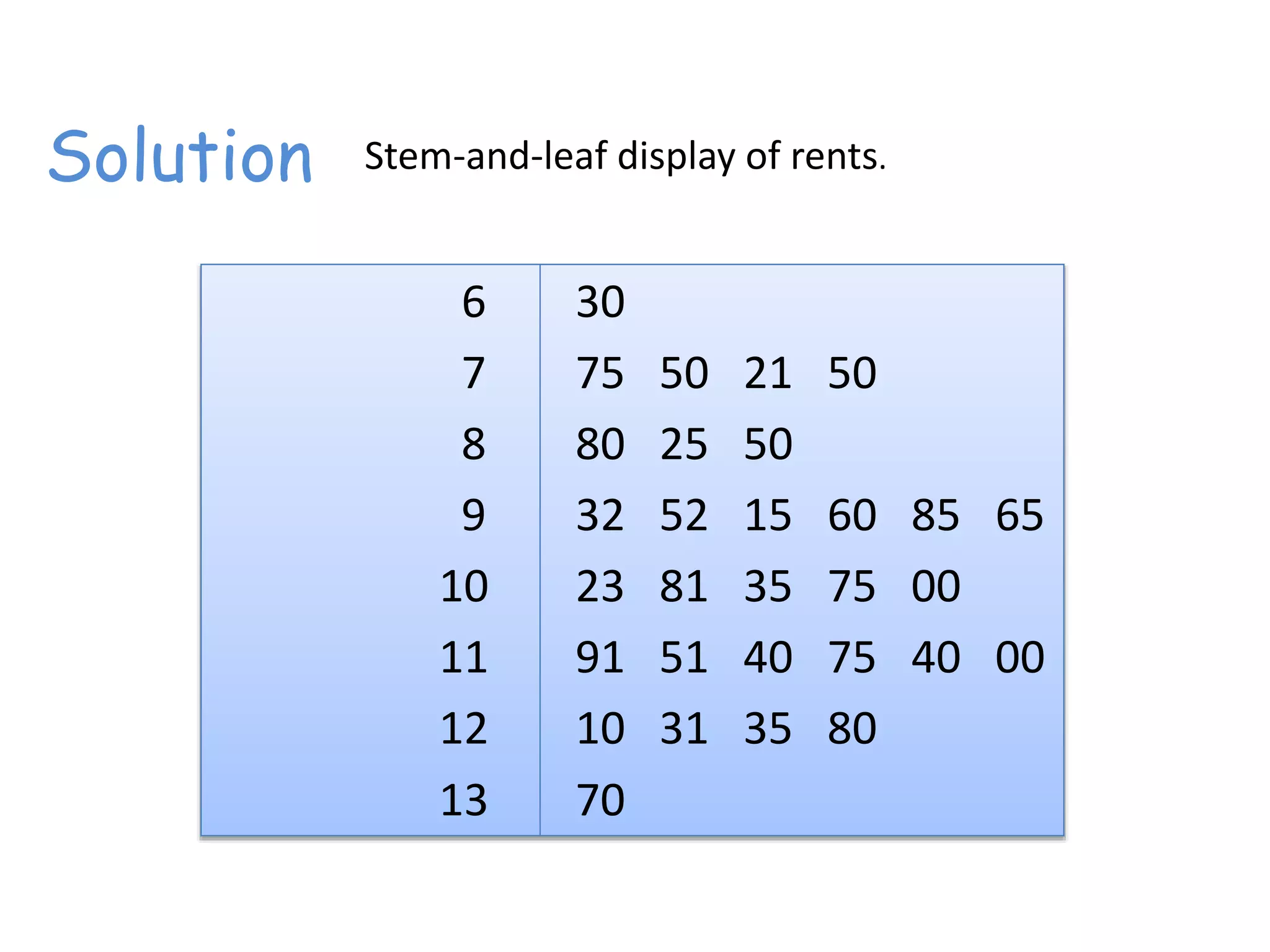
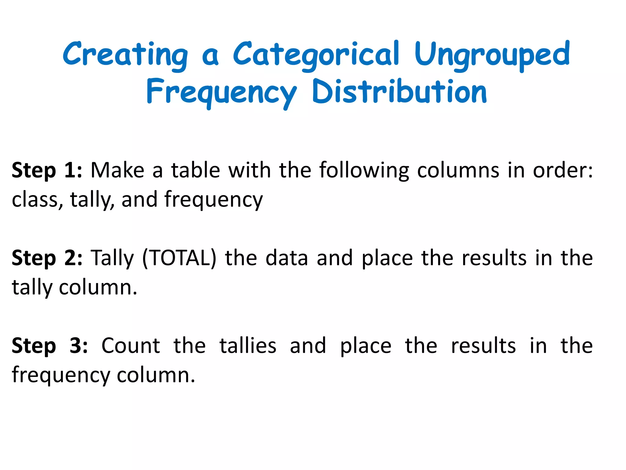
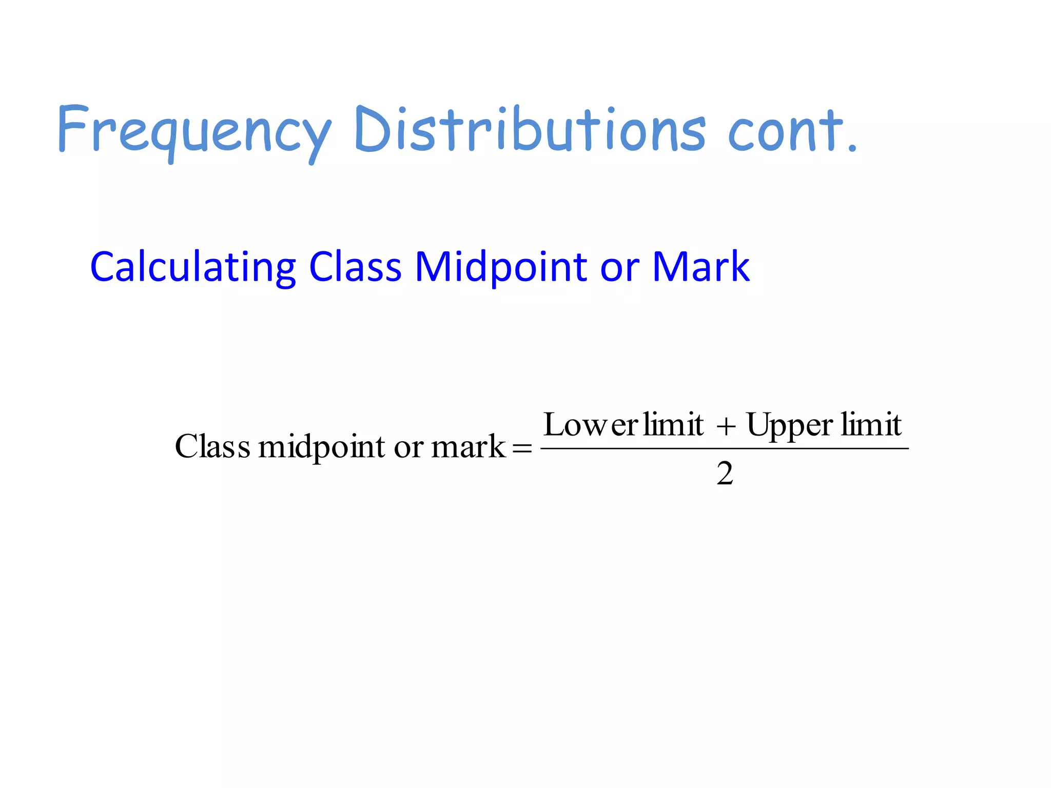
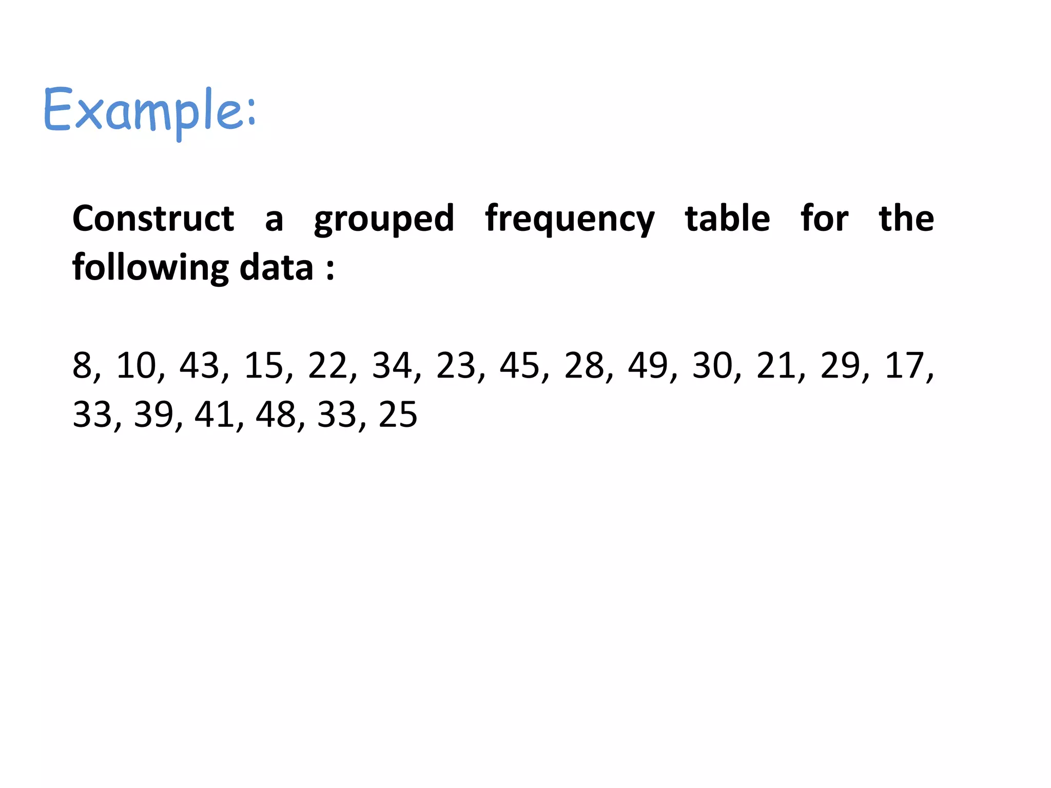
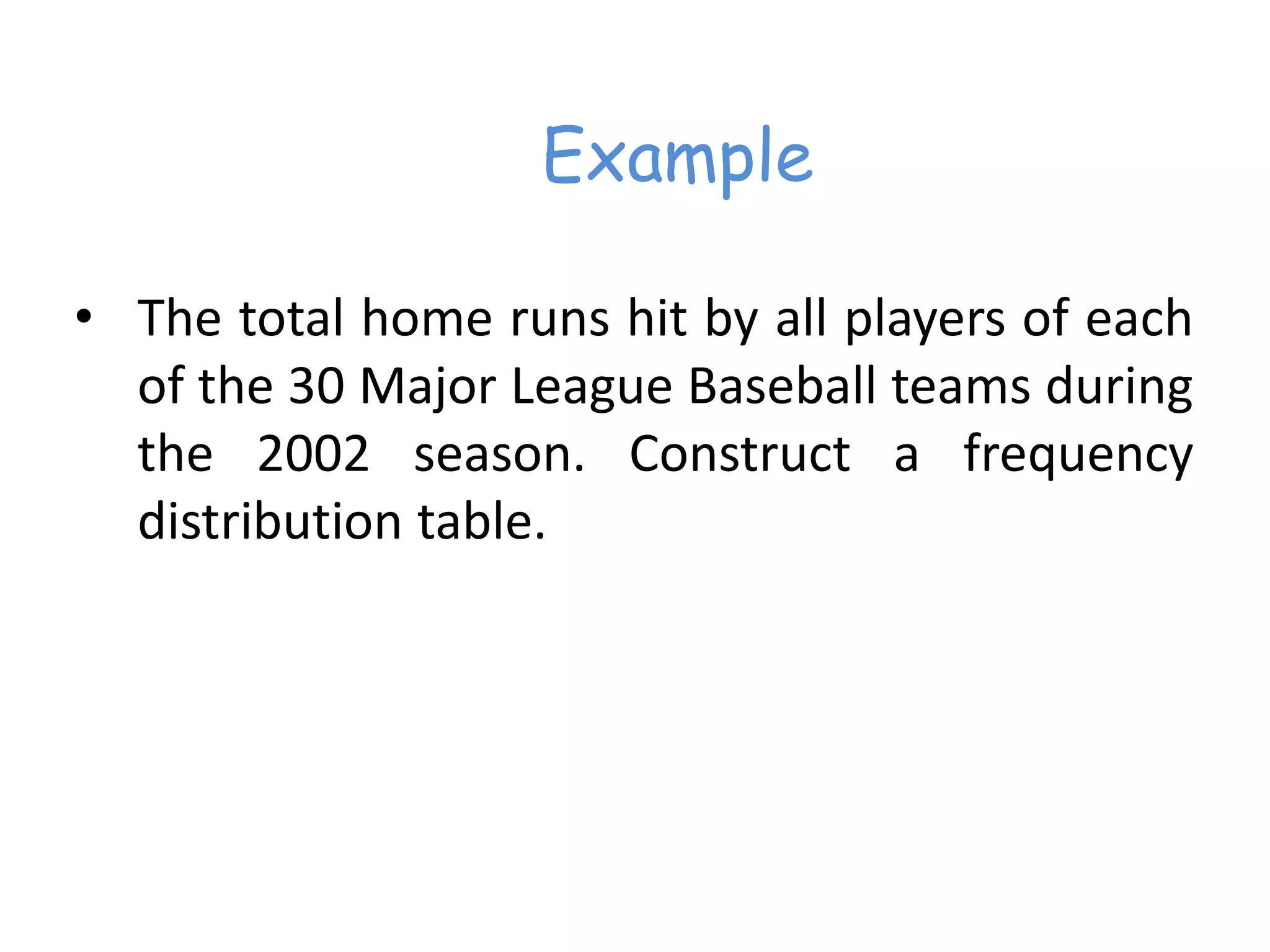
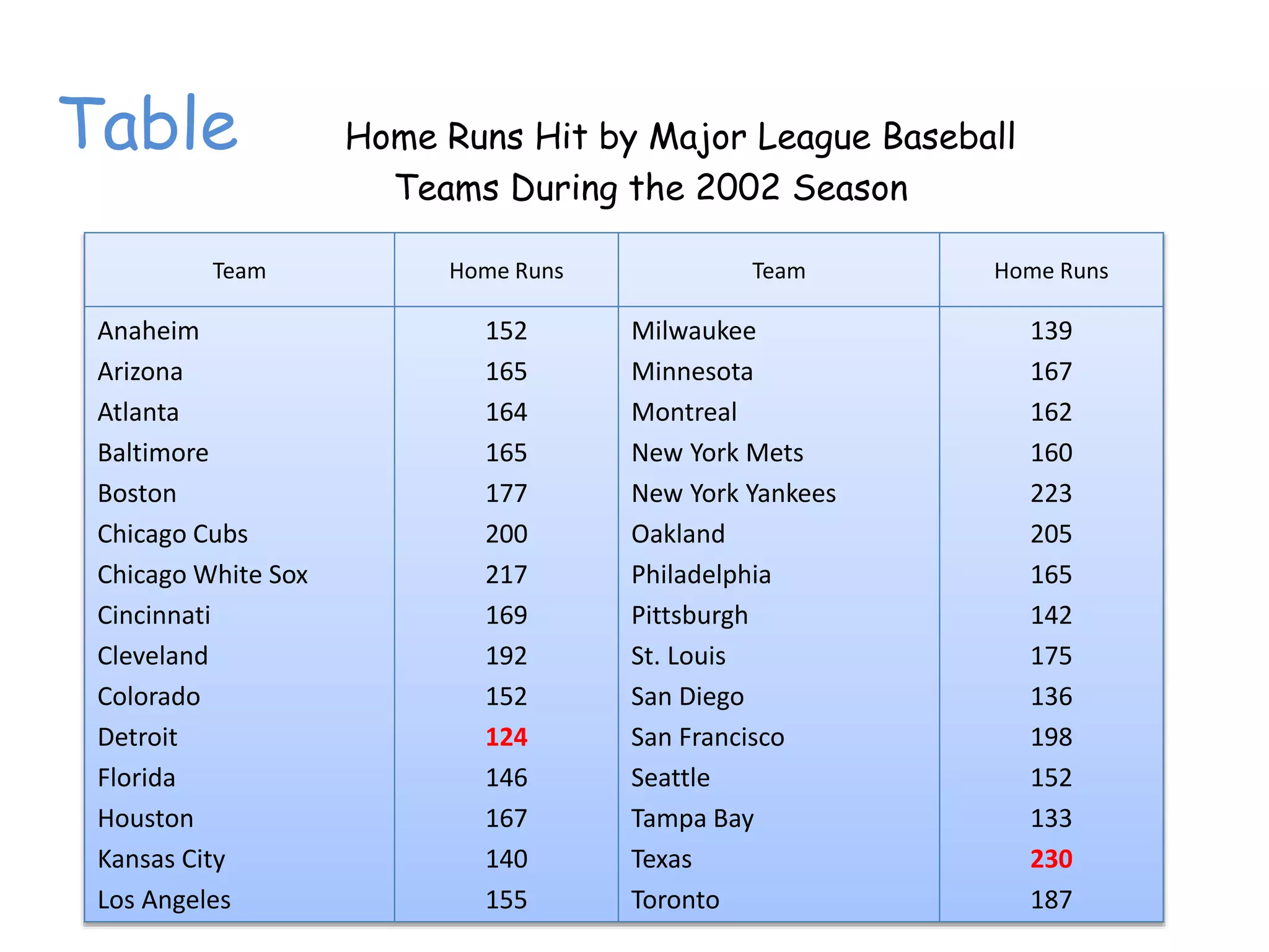
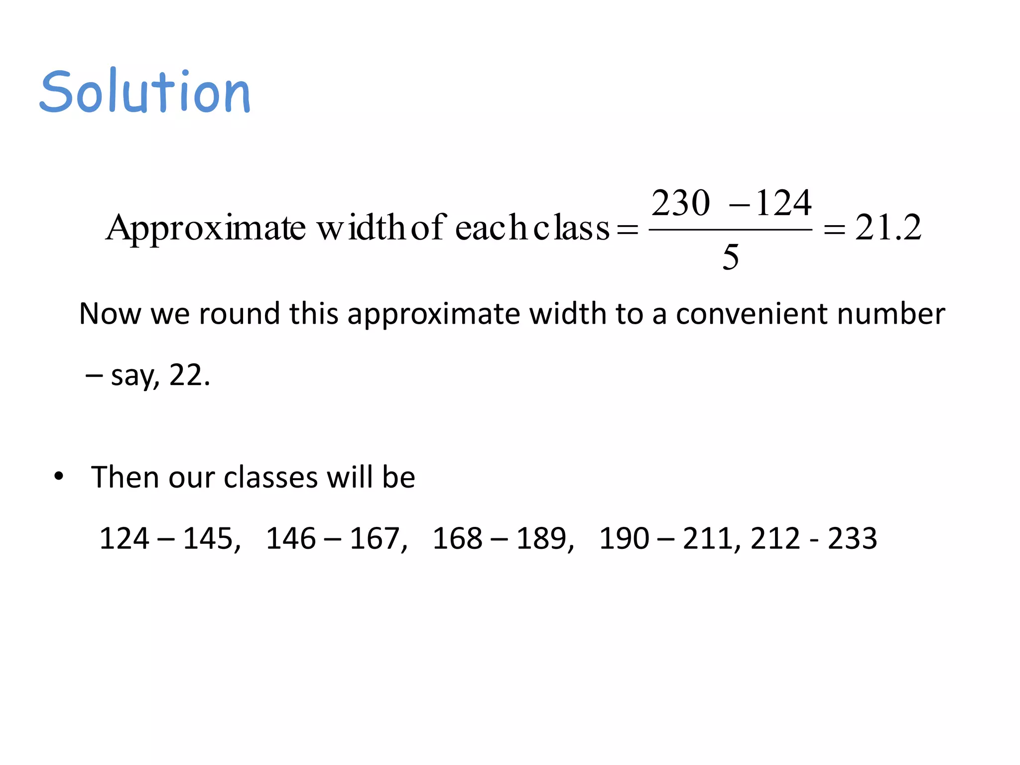
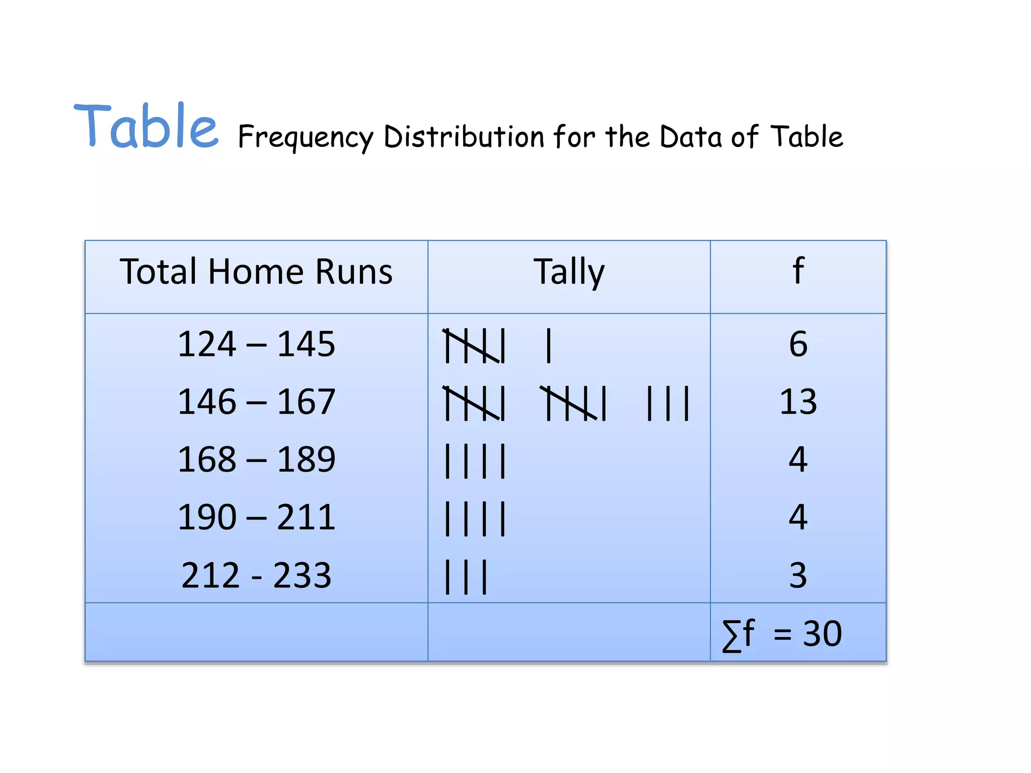
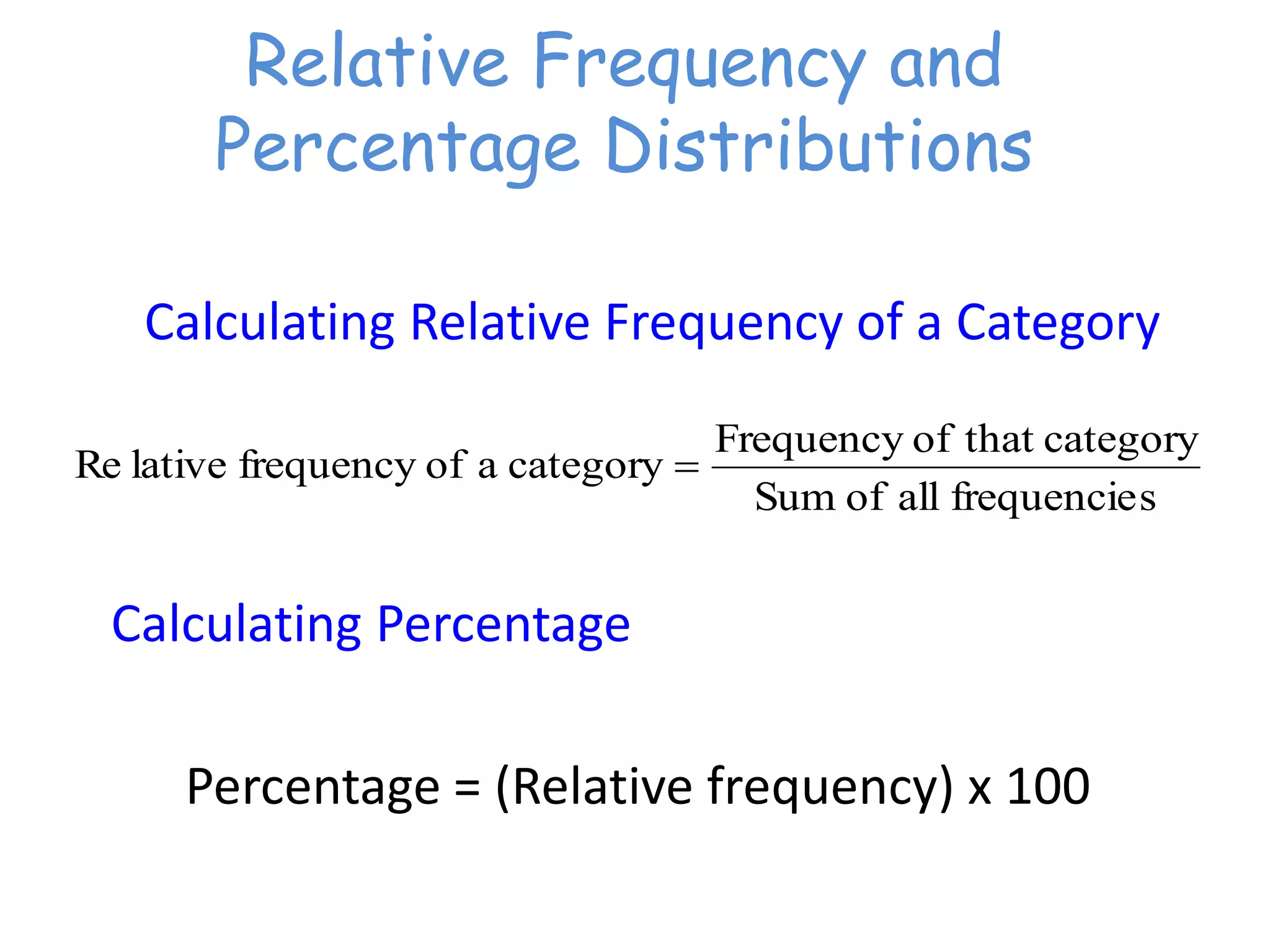
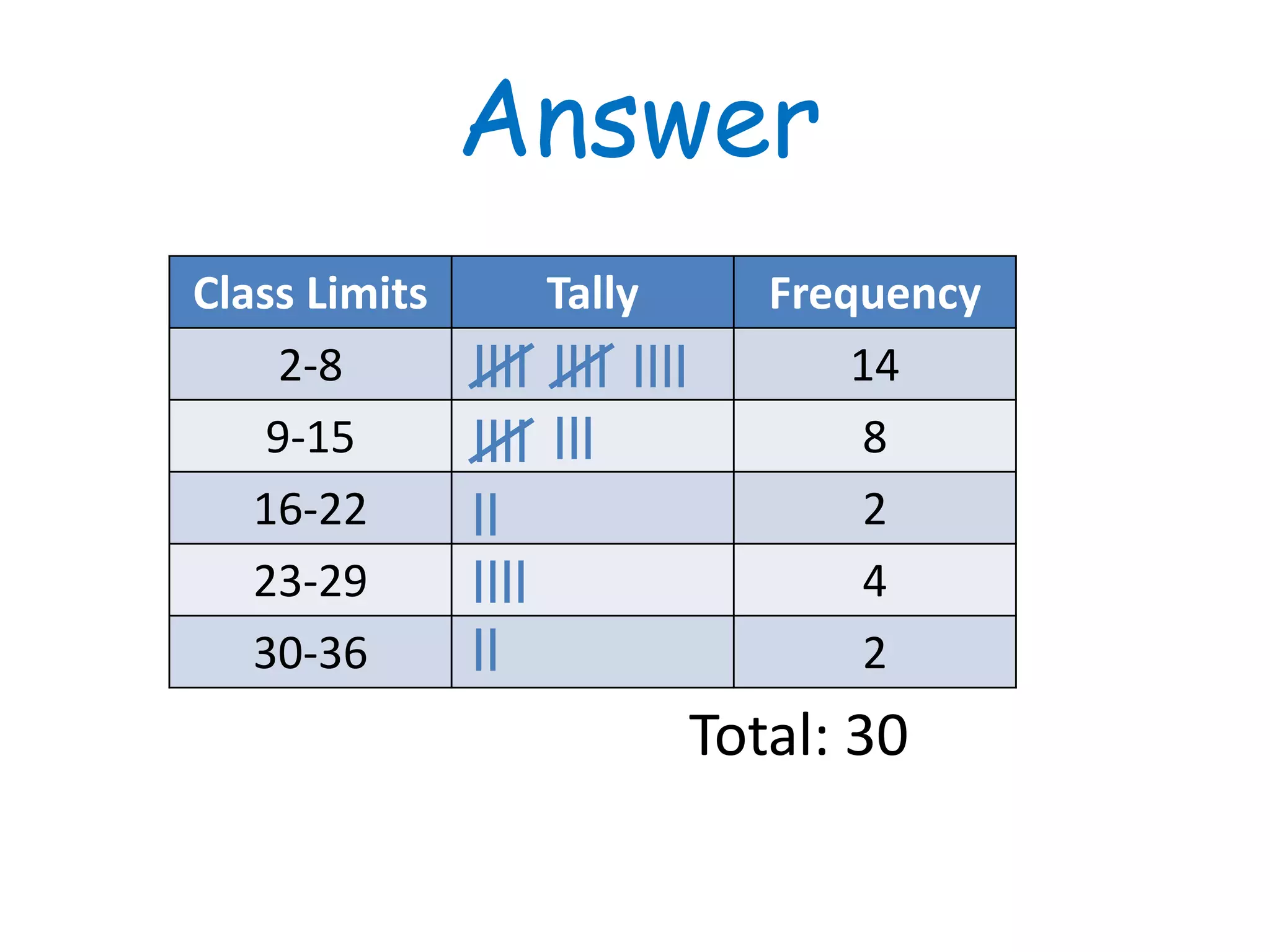
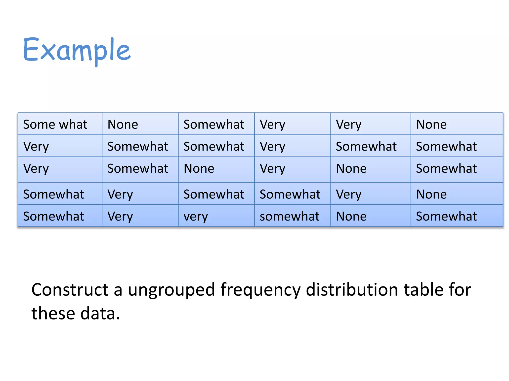
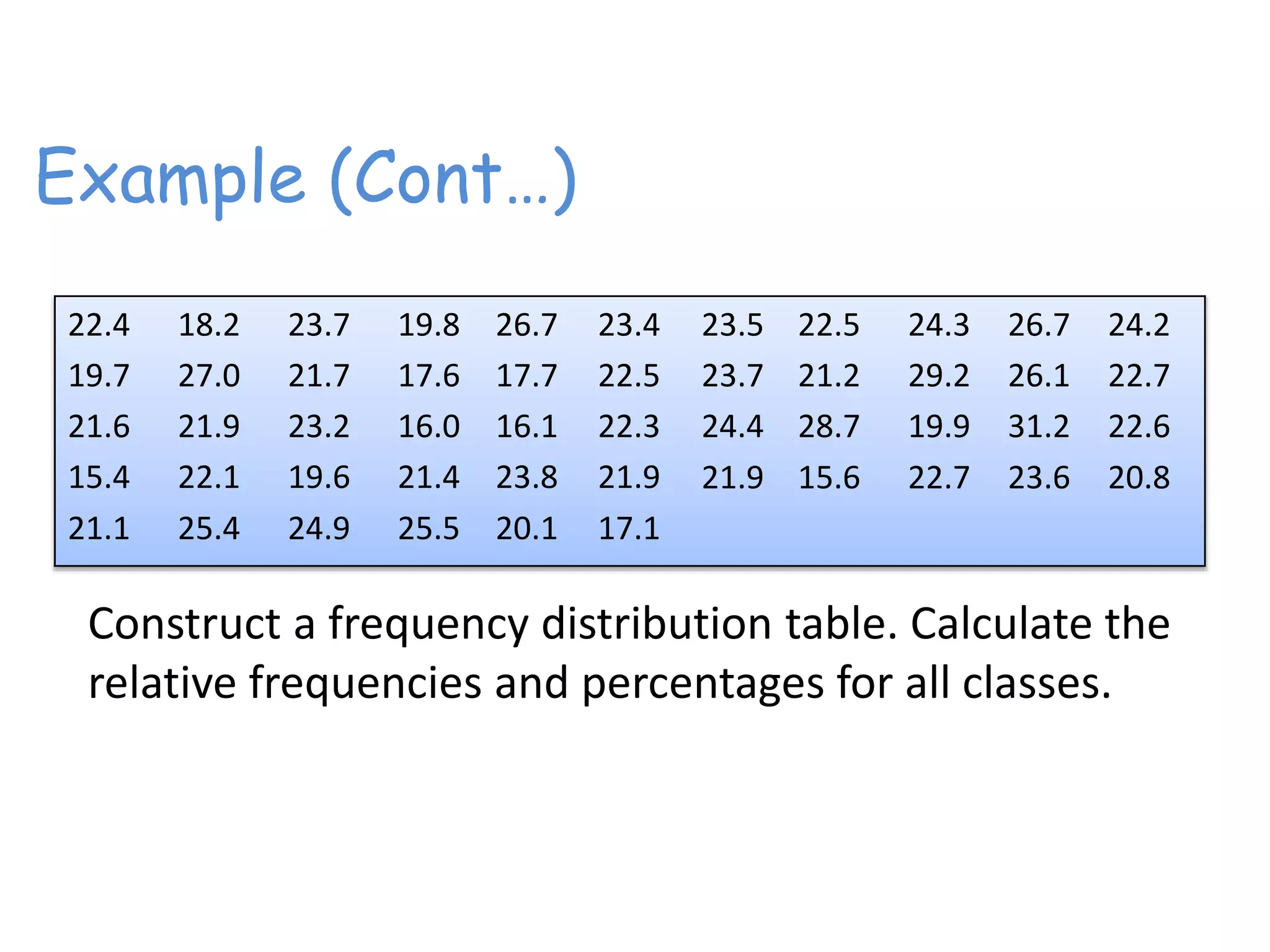
This document discusses frequency distributions and how to construct them from raw data. It provides examples of creating stem-and-leaf displays, frequency tables, relative frequency tables, and cumulative frequency tables from various data sets. Key concepts covered include class width, class boundaries, tallying data, and calculating relative frequencies and percentages. Overall, the document serves as a tutorial on how to organize and summarize data using various types of frequency distributions.

1. Frequency Distributions
BY UNSA SHAKIR

2. Example
The following are the scores of 30 college
students in a statistics test:
Construct a stem-and-leaf display.
75
69
83
52
72
84
80
81
77
96
61
64
65
76
71
79
86
87
71
79
72
87
68
92
93
50
57
95
92
98

3. Figure Stem-and-leaf display of test scores.
5
6
7
8
9
2 0 7
5 9 1 8 4
5 9 1 2 6 9 7 1 2
0 7 1 6 3 4 7
6 3 5 2 2 8

4. Example
The following data are monthly rents paid by a
sample of 30 households selected from a small city.
Construct a stem-and-leaf display for these data.
880
1210
1151
1081
985
630
721
1231
1175
1075
932
952
1023
850
1100
775
825
1140
1235
1000
750
750
915
1140
965
1191
1370
960
1035
1280

5. Solution
6
7
8
9
10
11
12
13
30
75 50 21 50
80 25 50
32 52 15 60 85 65
23 81 35 75 00
91 51 40 75 40 00
10 31 35 80
70
Stem-and-leaf display of rents.

6. Exercise
Develop your own Stem and Leaf Plot with the following
temperatures for June.
77 80 82 68 65 59 61
57 50 62 61 70 69 64
67 70 62 65 65 73 76
87 80 82 83 79 79 71
80 77

7. Example
0
1
2
3
4
5
6
7
8
6
1 7 9
2 6
2 4 7 8
1 5 6 9 9
3 6 8
2 4 4 5 7
5 6
The following stem-and-leaf display is prepared for the
number of hours that 25 students spent working on
computers during the last month.
Prepare a new stem-and-leaf display by grouping the stems.

8. Solution
0 – 2
3 – 5
6 – 8
6 * 1 7 9 * 2 6
2 4 7 8 * 1 5 6 9 9 * 3 6 8
2 4 4 5 7 * * 5 6
Grouped stem-and-leaf display.

9. Grouped DataVs Ungrouped Data
Ungrouped data – Data
that has not been
organized into groups.
Also called as raw data.
Grouped data - Data
that has been organized
into groups (into a
frequency distribution).
Data Frequency
2 – 4 5
5 – 7 6
8 – 10 10
11 – 13 8
14 – 16 4
17 – 19 3
Data Frequency
2 8
3 4
5 6
7 7
8 2
9 5

10. Step 1: Make a table with the following columns in order:
class, tally, and frequency
Step 2: Tally (TOTAL) the data and place the results in the
tally column.
Step 3: Count the tallies and place the results in the
frequency column.
Creating a Categorical Ungrouped
Frequency Distribution

11. Example:
Below is the marks of 35 students in English test (out of
10). Arrange these marks in tabular form using tally
marks. 5, 8, 7, 6, 10, 8, 2, 4, 6, 3, 7, 5, 8, 5, 1, 7, 4, 6, 3,
5, 2, 8, 4, 2, 6, 4, 2, 8, 9, 5, 4, 7, 5, 5, 8.

12. Example:
Let us consider the following data:
2, 3, 3, 5, 7, 9, 7, 8, 9, 9, 2, 5, 3, 9, 3, 2, 5, 9, 8,
7, 3, 5, 7, 9, 8, 5, 2, 3
Design frequency table for above data.

13. Class Tally Frequency
Total=
Example
These are the favorite colors of fifteen 2nd graders.
Red
Yellow
Green
Red
Blue
Blue
Red
Red
Green
Red
Green
Yellow
Red
Blue
Green

14. • When the range of the data is large, the data must be grouped
into classes
Grouped Frequency Distribution
41 104 112 118 87 95
105 57 107 67 78 125
109 99 105 99 101 92

15. Key Concept

16. • The class width is the range of the class.
• Can be found by subtracting the lower class limit of
one class from the upper class limit of the next
class
Class Width
Class width = Upper boundary – Lower boundary
# of classes

17. Frequency Distributions cont.
Calculating Class Midpoint or Mark
2
limitUpperlimitLower
markormidpointClass



18. Rule #1: Choose the classes
You will normally be told how many classes you need
Rule #2: Choose Class Width
ALWAYS round up to the next whole number
Rule #3: Mutually Exclusive
This means the class limits cannot overlap or be
contained in more than one class.
Rules For Grouped Data

19. Rule #4: Continuous
Even if there are no values in a class the class must be
included in the frequency distribution. There should be
no gaps in a frequency distribution.
(with the exception of a class with zero frequency)
Rule #5: Exhaustive
There should be enough classes to accommodate all of
the data
Rule #6: Equal Width
This avoids a distorted view of the data.
Rules For Grouped Data

20. Table Class Widths, and Class Midpoints
Class Limits Class Width Class Midpoint
400 to 600
601 to 800
801 to 1000
1001 to 1200
1201 to 1400
1401 to 1600
200
200
200
200
200
200
500
700.5
900.5
1100.5
1300.5
1500.5

21. Frequency Distributions
102 124 108 86 103 82
71 104 112 118 87 95
103 116 85 122 87 100
105 97 107 67 78 125
109 99 105 99 101 92
Make a frequency distribution table with five classes.
Minutes Spent on the Phone
Minimum value =
Maximum value =
67
125

22. Total=30
78
90
102
114
126
3
5
8
9
5
67
79
91
103
115
Class Limits Tally f
Construct a Frequency Distribution Table
Minimum = 67, Maximum = 125
Number of classes = 5
Class width = 11.6 = 12

23. Construct a grouped frequency table for the
following data :
8, 10, 43, 15, 22, 34, 23, 45, 28, 49, 30, 21, 29, 17,
33, 39, 41, 48, 33, 25
Example:

24. Example
• The total home runs hit by all players of each
of the 30 Major League Baseball teams during
the 2002 season. Construct a frequency
distribution table.

25. Table Home Runs Hit by Major League Baseball
Teams During the 2002 Season
Team Home Runs Team Home Runs
Anaheim
Arizona
Atlanta
Baltimore
Boston
Chicago Cubs
Chicago White Sox
Cincinnati
Cleveland
Colorado
Detroit
Florida
Houston
Kansas City
Los Angeles
152
165
164
165
177
200
217
169
192
152
124
146
167
140
155
Milwaukee
Minnesota
Montreal
New York Mets
New York Yankees
Oakland
Philadelphia
Pittsburgh
St. Louis
San Diego
San Francisco
Seattle
Tampa Bay
Texas
Toronto
139
167
162
160
223
205
165
142
175
136
198
152
133
230
187

26. Solution
2.21
5
124230
classeachofwidtheApproximat 


Now we round this approximate width to a convenient number
– say, 22.
• Then our classes will be
124 – 145, 146 – 167, 168 – 189, 190 – 211, 212 - 233

27. Table Frequency Distribution for the Data of Table
Total Home Runs Tally f
124 – 145
146 – 167
168 – 189
190 – 211
212 - 233
|||| |
|||| |||| |||
||||
||||
|||
6
13
4
4
3
∑f = 30

28. Relative Frequency and
Percentage Distributions
Calculating Relative Frequency of a Category
sfrequencieallofSum
categorythatofFrequency
categoryaoffrequencylativeRe 
Calculating Percentage
Percentage = (Relative frequency) x 100

29. Solution
Total Home
Runs
f Relative
Frequency
Percentage
124 – 145
146 – 167
168 – 189
190 – 211
212 - 233
6
13
4
4
3
.200
.433
.133
.133
.100
20.0
43.3
13.3
13.3
10.0
∑f = 30 Sum = .999 Sum = 99.9%
Table Relative Frequency and Percentage Distributions for Table

30. After conducting a survey of 30 of your classmates, you
are left with the following set of data on how many days
off each employee has taken this year:
Construct a Frequency Table. Assume you want to divide the
data into 5 different classes.
Example
7, 8, 9, 4, 10, 36, 19, 9, 26, 5, 11, 6, 2, 9, 10,
8, 16, 29, 7, 9, 8, 25, 4, 27, 8, 7, 6, 10, 34, 8

31. Answer
Class Limits Tally Frequency
2-8 14
9-15 8
16-22 2
23-29 4
30-36 2
Total: 30

32. Example
Some what None Somewhat Very Very None
Very Somewhat Somewhat Very Somewhat Somewhat
Very Somewhat None Very None Somewhat
Somewhat Very Somewhat Somewhat Very None
Somewhat Very very somewhat None Somewhat
Construct a ungrouped frequency distribution table for
these data.

33. Solution
Stress on Job Tally Frequency (f)
Very
Somewhat
None
|||| ||||
|||| |||| ||||
|||| |
10
14
6
Sum = 30
Table Frequency Distribution of Stress on Job

34. Example
Stress on
Job
Frequency (f)
Relative Frequency Percentage
Very
Somewhat
None
10
14
6
10/30 = .333
14/30 = .467
6/30 = .200
.333(100) = 33.3
.467(100) = 46.7
.200(100) = 20.0
Sum = 30 Sum = 1.00 Sum = 100
Table Relative Frequency and Percentage Distributions of Stress on Job
• Determine the relative frequency and percentage for
the data in previous Table

35. Example
The following data give the average travel time
from home to work (in minutes) for 50 states. The
data are based on a sample survey of 700,000
households conducted by the Census Bureau (USA
TODAY, August 6, 2001).

36. Example (Cont…)
22.4
19.7
21.6
15.4
21.1
18.2
27.0
21.9
22.1
25.4
23.7
21.7
23.2
19.6
24.9
19.8
17.6
16.0
21.4
25.5
26.7
17.7
16.1
23.8
20.1
23.4
22.5
22.3
21.9
17.1
23.5
23.7
24.4
21.9
22.5
21.2
28.7
15.6
24.3
29.2
19.9
22.7
26.7
26.1
31.2
23.6
24.2
22.7
22.6
20.8
Construct a frequency distribution table. Calculate the
relative frequencies and percentages for all classes.

37. Solution
63.2
6
4.152.31
classeachofwidtheApproximat 



38. Solution
Class Boundaries f
Relative
Frequency
Percentage
15 to less than 18
18 to less than 21
21 to less than 24
24 to less than 27
27 to less than 30
30 to less than 33
7
7
23
9
3
1
.14
.14
.46
.18
.06
.02
14
14
46
18
6
2
Σf = 50 Sum = 1.00 Sum = 100%
Table Frequency, Relative Frequency, and Percentage Distributions
of Average Travel Time to Work

39. Example
The administration in a large city wanted to know the
distribution of vehicles owned by households in that city. A
sample of 40 randomly selected households from this city
produced the following data on the number of vehicles owned:
5 1 1 2 0 1 1 2 1 1
1 3 3 0 2 5 1 2 3 4
2 1 2 2 1 2 2 1 1 1
4 2 1 1 2 1 1 4 1 3
• Construct a frequency distribution table for these data, and
draw a bar graph.

40. Solution
Vehicles Owned
Number of
Households (f)
0
1
2
3
4
5
2
18
11
4
3
2
Σf = 40
Table Frequency Distribution of Vehicles Owned

41. Figure Bar graph for Table
0
2
4
6
8
10
12
14
16
18
20
No Car 1 Car 2 Cars 3 Cars 4 Cars 5 Cars
Vehicles owned
Frequency

42. CUMULATIVE FREQUENCY
DISTRIBUTIONS
Definition
A cumulative frequency distribution gives the
total number of values that fall below the upper
boundary of each class.

43. Example
Using the frequency distribution of Table in
ptrvious example, reproduced in the next slide,
prepare a cumulative frequency distribution for t
he home runs hit by Major League Baseball
teams during the 2002 season.

44. Example
Total Home Runs f
124 – 145
146 – 167
168 – 189
190 – 211
212 - 233
6
13
4
4
3

45. Solution
Class Limits f Cumulative Frequency
124 – 145
124 – 167
124 – 189
124 – 211
124 – 233
6
13
4
4
3
6
6 + 13 = 19
6 + 13 + 4 = 23
6 + 13 + 4 + 4 = 27
6 + 13 + 4 + 4 + 3 = 30
Table Cumulative Frequency Distribution of Home Runs by Baseball Teams

46. CUMULATIVE FREQUENCY
DISTRIBUTIONS cont.
Calculating Cumulative Relative Frequency and
Cumulative Percentage
100frequency)relativee(CumulativpercentageCumulative
setdatain thensobservatioTotal
classaoffrequencyCumulative
frequencyrelativeCumulative



47. Table Cumulative Relative Frequency and
Cumulative Percentage Distributions for
Home Runs Hit by baseball Teams
Class Limits
Cumulative
Relative Frequency
Cumulative Percentage
124 – 145
124 – 167
124 – 189
124 – 211
124 - 233
6/30 = .200
19/30 = .633
23/30 = .767
27/30 = .900
30/30 = 1.00
20.0
63.3
76.7
90.0
100.0

48. CUMULATIVE FREQUENCY
DISTRIBUTIONS cont.
Definition
An ogive is a curve drawn for the cumulative
frequency distribution by joining with straight lines
the dots marked above the upper boundaries of
classes at heights equal to the cumulative
frequencies of respective classes.

49. Figure Ogive for the cumulative frequency
distribution in Table
123.5 145.5 167.5 189.5 211.5 233.5
30
25
20
15
10
5
Total home runs
Cumulativefrequency

50. Shape
• A graph shows the shape of the distribution.
• A distribution is symmetrical if the left side of the
graph is (roughly) a mirror image of the right side.
• One example of a symmetrical distribution is the
bell-shaped normal distribution.
• On the other hand, distributions are skewed when
scores pile up on one side of the distribution,
leaving a "tail" of a few extreme values on the other
side.

51. Positively and Negatively
Skewed Distributions
• In a positively skewed distribution, the scores
tend to pile up on the left side of the
distribution with the tail tapering off to the
right.
• In a negatively skewed distribution, the
scores tend to pile up on the right side and
the tail points to the left.