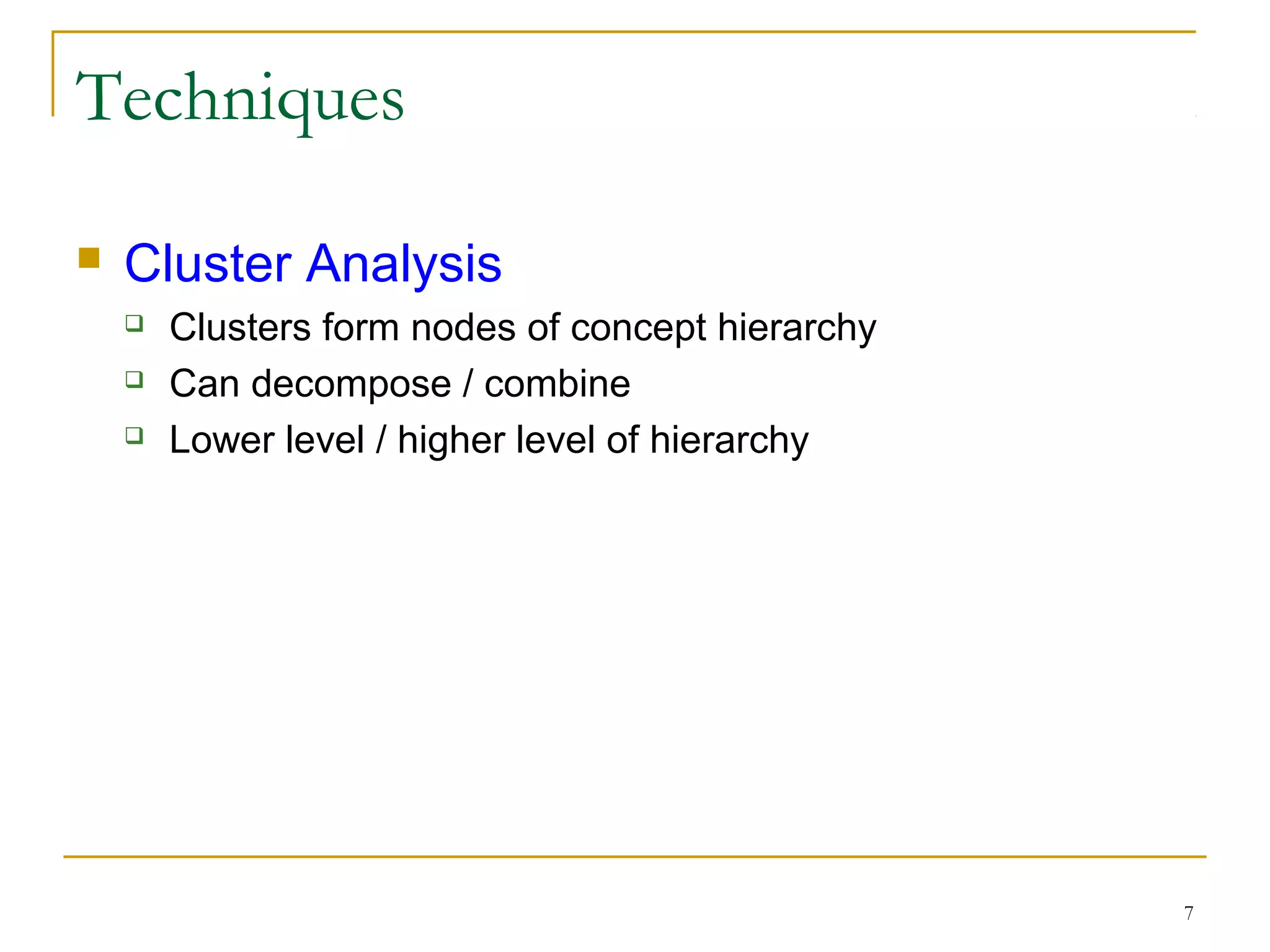
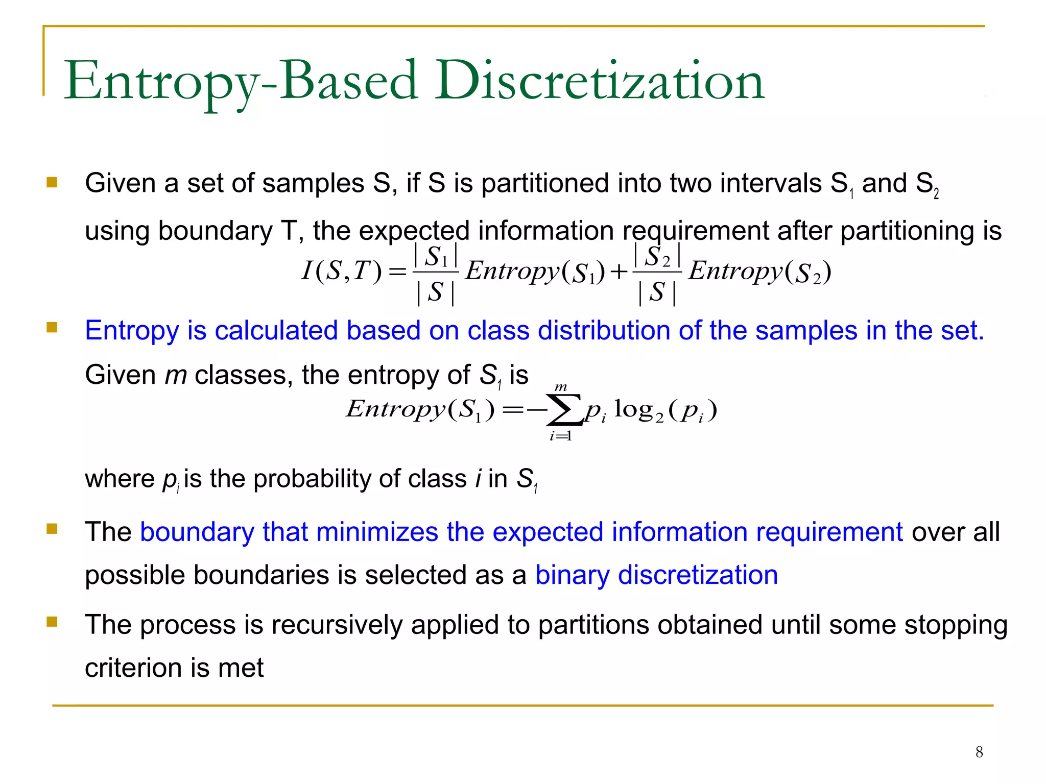
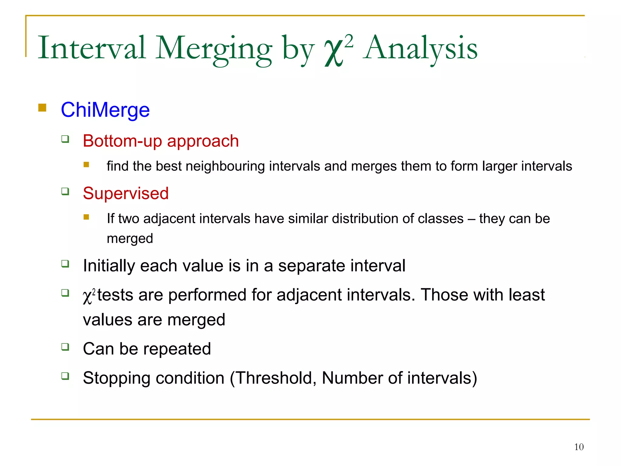
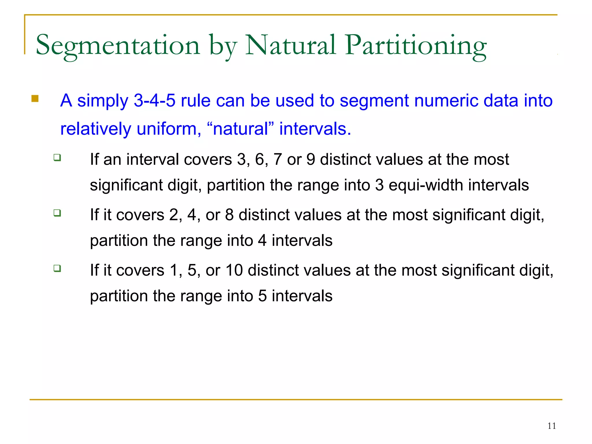
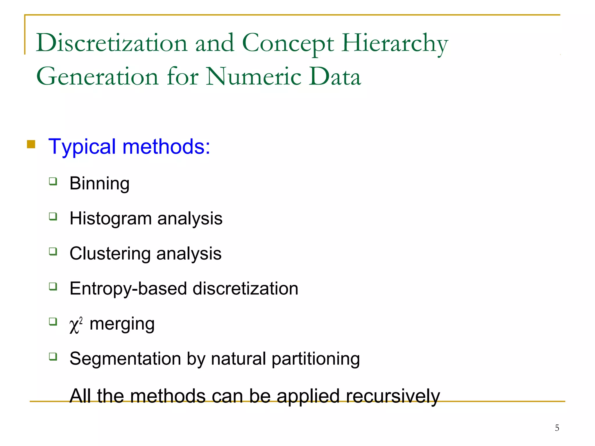
1. Discretization involves dividing the range of continuous attributes into intervals to reduce data size. Concept hierarchy formation recursively groups low-level concepts like numeric values into higher-level concepts like age groups. 2. Common techniques for discretization and concept hierarchy generation include binning, histogram analysis, clustering analysis, and entropy-based discretization. These techniques can be applied recursively to generate hierarchies. 3. Discretization and concept hierarchies reduce data size, provide more meaningful interpretations, and make data mining and analysis easier.

1. 1
Discretization and Concept
Hierarchy Generation

2. 2
Discretization
 Types of attributes:
 Nominal — values from an unordered set, e.g., color, profession
 Ordinal — values from an ordered set, e.g., military or academic
rank
 Continuous — real numbers, e.g., integer or real numbers
 Discretization:
 Divide the range of a continuous attribute into intervals
 Reduce data size by discretization

3. 3
Discretization and Concept Hierarchy
 Discretization
 Reduce the number of values for a given continuous attribute
by dividing the range of the attribute into intervals
 Interval labels can then be used to replace actual data values
 Supervised vs. unsupervised
 Split (top-down) vs. merge (bottom-up)
 Discretization can be performed recursively on an attribute

4. 4
Concept hierarchy
 Concept hierarchy formation
 Recursively reduce the data by collecting and replacing low level
concepts (such as numeric values for age) by higher level
concepts (such as young, middle-aged, or senior)
 Detail lost
 More meaningful
 Easier to interpret
 Mining becomes easier
 Several concept hierarchies can be defined for the same
attribute
 Manual / Implicit

5. 5
Discretization and Concept Hierarchy
Generation for Numeric Data
 Typical methods:
 Binning
 Histogram analysis
 Clustering analysis
 Entropy-based discretization
 χ2
merging
 Segmentation by natural partitioning
All the methods can be applied recursively

6. 6
Techniques
 Binning
 Distribute values into bins
 Replace by bin mean / median
 Recursive application – leads to concept hierarchies
 Unsupervised technique
 Histogram Analysis
 Data Distribution – Partition
 Equiwidth – (0-100], (100-200], …
 Equidepth
 Recursive
 Minimum Interval size
 Unsupervised

7. 7
Techniques
 Cluster Analysis
 Clusters form nodes of concept hierarchy
 Can decompose / combine
 Lower level / higher level of hierarchy

8. 8
Entropy-Based Discretization
 Given a set of samples S, if S is partitioned into two intervals S1 and S2
using boundary T, the expected information requirement after partitioning is
 Entropy is calculated based on class distribution of the samples in the set.
Given m classes, the entropy of S1 is
where pi is the probability of class i in S1
 The boundary that minimizes the expected information requirement over all
possible boundaries is selected as a binary discretization
 The process is recursively applied to partitions obtained until some stopping
criterion is met
)(
||
||
)(
||
||
),( 2
2
1
1
SEntropy
S
S
SEntropy
S
S
TSI +=
∑=
−=
m
i
ii ppSEntropy
1
21 )(log)(

9. 9
 Reduces data size
 Class information is considered
 Improves accuracy
Entropy-Based Discretization

10. 10
Interval Merging by χ2
Analysis
 ChiMerge
 Bottom-up approach
 find the best neighbouring intervals and merges them to form larger intervals
 Supervised
 If two adjacent intervals have similar distribution of classes – they can be
merged
 Initially each value is in a separate interval
 χ2
tests are performed for adjacent intervals. Those with least
values are merged
 Can be repeated
 Stopping condition (Threshold, Number of intervals)

11. 11
Segmentation by Natural Partitioning
 A simply 3-4-5 rule can be used to segment numeric data into
relatively uniform, “natural” intervals.
 If an interval covers 3, 6, 7 or 9 distinct values at the most
significant digit, partition the range into 3 equi-width intervals
 If it covers 2, 4, or 8 distinct values at the most significant digit,
partition the range into 4 intervals
 If it covers 1, 5, or 10 distinct values at the most significant digit,
partition the range into 5 intervals

12. 12
 Outliers could be present
 Consider only the majority values
 5th
percentile – 95th
percentile
Segmentation by Natural Partitioning

13. 13
Example of 3-4-5 Rule
(-$400 -$5,000)
(-$400 - 0)
(-$400 -
-$300)
(-$300 -
-$200)
(-$200 -
-$100)
(-$100 -
0)
(0 - $1,000)
(0 -
$200)
($200 -
$400)
($400 -
$600)
($600 -
$800) ($800 -
$1,000)
($2,000 - $5, 000)
($2,000 -
$3,000)
($3,000 -
$4,000)
($4,000 -
$5,000)
($1,000 - $2, 000)
($1,000 -
$1,200)
($1,200 -
$1,400)
($1,400 -
$1,600)
($1,600 -
$1,800)
($1,800 -
$2,000)
msd=1,000 Low=-$1,000 High=$2,000Step 2:
Step 4:
Step 1: -$351 -$159 profit $1,838 $4,700
Min Low (i.e, 5%-tile) High(i.e, 95%-tile) Max
count
(-$1,000 - $2,000)
(-$1,000 - 0) (0 -$ 1,000)
Step 3:
($1,000 - $2,000)

14. 14
Concept Hierarchy Generation for
Categorical Data
 Specification of a partial ordering of attributes explicitly at
the schema level by users or experts
 User / Expert defines hierarchy
 Street < city < state < country
 Specification of a portion of a hierarchy by explicit data
grouping
 Manual
 Intermediate level information specified
 Industrial, Agricultural..

15. 15
Concept Hierarchy Generation for
Categorical Data
 Specification of a set of attributes but not their partial
ordering
 Automatically inferring the hierarchy
 Heuristic rule
 High level concepts contain a smaller number of values
 Specification of only a partial set of attributes
 Embedding data semantics
 Attributes with tight semantic connections are pinned together