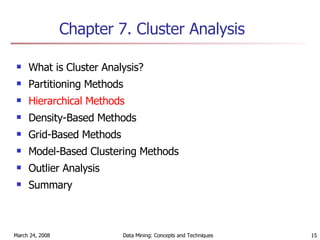
Cluster Analysis ©Jiawei Han and Micheline Kamber http://www-sal.cs.uiuc.edu/~hanj/bk2/ Chp 7 modified by Donghui Zhang
Chapter 7.  Cluster Analysis What is Cluster Analysis? Partitioning Methods Hierarchical Methods Density-Based Methods Grid-Based Methods Model-Based Clustering Methods Outlier Analysis Summary
What is Cluster Analysis? Cluster: a collection of data objects Similar to one another within the same cluster Dissimilar to the objects in other clusters Cluster analysis Grouping a set of data objects into clusters Clustering is  unsupervised classification : no predefined classes Typical applications As a  stand-alone tool  to get insight into data distribution  As a  preprocessing step  for other algorithms
General Applications of Clustering  Pattern Recognition Spatial Data Analysis  create thematic maps in GIS by clustering feature spaces detect spatial clusters and explain them in spatial data mining Image Processing Economic Science (especially market research) WWW Document classification Cluster Weblog data to discover groups of similar access patterns
Examples of Clustering Applications Marketing:  Help marketers discover distinct groups in their customer bases, and then use this knowledge to develop targeted marketing programs Land use:  Identification of areas of similar land use in an earth observation database Insurance:  Identifying groups of motor insurance policy holders with a high average claim cost City-planning:  Identifying groups of houses according to their house type, value, and geographical location Earth-quake studies:  Observed earth quake epicenters should be clustered along continent faults
What Is Good Clustering? A  good clustering  method will produce high quality clusters with high  intra-class  similarity low  inter-class  similarity  The  quality  of a clustering result depends on both the similarity measure used by the method and its implementation. The  quality  of a clustering method is also measured by its ability to discover some or all of the  hidden  patterns.
Requirements of Clustering in Data Mining  Scalability Ability to deal with different types of attributes Discovery of clusters with arbitrary shape Minimal requirements for domain knowledge to determine input parameters Able to deal with noise and outliers Insensitive to order of input records High dimensionality Incorporation of user-specified constraints Interpretability and usability
Major Clustering Approaches Partitioning algorithms : Construct various partitions and then evaluate them by some criterion Hierarchy algorithms : Create a hierarchical decomposition of the set of data (or objects) using some criterion Density-based : based on connectivity and density functions Grid-based : based on a multiple-level granularity structure Model-based : A model is hypothesized for each of the clusters and the idea is to find the best fit of that model to each other
Chapter 7.  Cluster Analysis What is Cluster Analysis? Partitioning Methods Hierarchical Methods Density-Based Methods Grid-Based Methods Model-Based Clustering Methods Outlier Analysis Summary
Partitioning Algorithms: Basic Concept Partitioning method:  Construct a partition of a database  D  of  n  objects into a set of  k  clusters Given a  k , find a partition of  k clusters  that optimizes the chosen partitioning criterion Global optimal: exhaustively enumerate all partitions Heuristic methods:  k-means  and  k-medoids  algorithms k-means  (MacQueen’67): Each cluster is represented by the center of the cluster k-medoids  or PAM (Partition around medoids) (Kaufman & Rousseeuw’87): Each cluster is represented by one of the objects in the cluster
The  K-Means  Clustering Method   Pick  k  objects as initial seed points Assign each object to the cluster with the nearest seed point  Re-compute each seed point as the centroid (or mean point) of its cluster Go back to Step 2, stop when no more new assignment
The  K-Means  Clustering Method   Example 0 1 2 3 4 5 6 7 8 9 10 0 1 2 3 4 5 6 7 8 9 10 0 1 2 3 4 5 6 7 8 9 10 0 1 2 3 4 5 6 7 8 9 10 Assign each objects to most similar center 0 1 2 3 4 5 6 7 8 9 10 0 1 2 3 4 5 6 7 8 9 10 Update the cluster means 0 1 2 3 4 5 6 7 8 9 10 0 1 2 3 4 5 6 7 8 9 10 Update the cluster means K=2 Arbitrarily choose K object as initial cluster center reassign
Comments on the  K-Means  Method Strength:   Relatively efficient :  O ( tkn ), where  n  is # objects,  k  is # clusters, and  t  is # iterations. Normally,  k ,  t  <<  n . Comparing: PAM: O(k(n-k) 2  ), CLARA: O(ks 2  + k(n-k)) Comment:  Often terminates at a  local optimum . The  global optimum  may be found using techniques such as:  deterministic annealing  and  genetic algorithms Weakness Applicable only when  mean  is defined, then what about categorical data? Need to specify  k,  the  number  of clusters, in advance Unable to handle noisy data and  outliers Not suitable to discover clusters with  non-convex shapes
Variations of the  K-Means  Method A few variants of the  k-means  which differ in Selection of the initial  k  means Dissimilarity calculations Strategies to calculate cluster means K-Medoids:  Instead of taking the  mean  value, use  medoid  (the  most centrally located  object in a cluster). can handle outliers!
Chapter 7.  Cluster Analysis What is Cluster Analysis? Partitioning Methods Hierarchical Methods Density-Based Methods Grid-Based Methods Model-Based Clustering Methods Outlier Analysis Summary
Hierarchical Clustering Use distance matrix as clustering criteria.  This method does not require the number of clusters  k  as an input, but needs a termination condition  Step 0 Step 1 Step 2 Step 3 Step 4 b d c e a a b d e c d e a b c d e Step 4 Step 3 Step 2 Step 1 Step 0 agglomerative (AGNES) divisive (DIANA)
AGNES (Agglomerative Nesting) Introduced in Kaufmann and Rousseeuw (1990) Implemented in statistical analysis packages, e.g., Splus Use the Single-Link method and the dissimilarity matrix.  Merge nodes that have the least dissimilarity Go on in a non-descending fashion Eventually all nodes belong to the same cluster
A  Dendrogram  Shows How the Clusters are Merged Hierarchically Decompose data objects into a several levels of nested partitioning ( tree  of clusters), called a  dendrogram .  A  clustering  of the data objects is obtained by  cutting  the dendrogram at the desired level, then each  connected component  forms a cluster.
DIANA (Divisive Analysis) Introduced in Kaufmann and Rousseeuw (1990) Implemented in statistical analysis packages, e.g., Splus Inverse order of AGNES Eventually each node forms a cluster on its own
More on Hierarchical Clustering Methods Major weakness of agglomerative clustering methods do not scale  well: time complexity of at least  O ( n 2 ), where  n  is the number of total objects can never undo what was done previously Integration of hierarchical with distance-based clustering BIRCH (1996) : uses CF-tree and incrementally adjusts the quality of sub-clusters CURE (1998 ): selects well-scattered points from the cluster and then shrinks them towards the center of the cluster by a specified fraction CHAMELEON (1999) : hierarchical clustering using dynamic modeling
BIRCH (1996) Birch: Balanced Iterative Reducing and Clustering using Hierarchies,  by Zhang, Ramakrishnan, Livny (SIGMOD’96) Incrementally construct a CF (Clustering Feature) tree, a hierarchical data structure for multiphase clustering Phase 1: scan DB to build an initial in-memory CF tree (a multi-level compression of the data that tries to preserve the inherent clustering structure of the data)  Phase 2: use an arbitrary clustering algorithm to cluster the leaf nodes of the CF-tree  Scales linearly : finds a good clustering with a single scan and improves the quality with a few additional scans Weakness:  handles only numeric data, and sensitive to the order of the data record. Balanced Iterative Reducing and Clustering using Hierarchies
Clustering Feature Vector Clustering Feature:   CF = (N, LS, SS) N :  Number of data points LS:   N i=1  X i SS:   N i=1  (X i  ) 2 CF = (5, (16,30),244) (3,4) (2,6) (4,5) (4,7) (3,8)
Some Characteristics of CF Two CF can be aggregated. Given CF1=(N1, LS1, SS1), CF2 = (N2, LS2, SS2), If combined into one cluster, CF=(N1+N2, LS1+LS2, SS1+SS2). The centroid and radius can both be computed from CF. centroid is the center of the cluster radius is the average distance between an object and the centroid. how?
Some Characteristics of CF
CF-Tree in BIRCH Clustering feature:  summary of the statistics for a given subcluster: the 0-th, 1st and 2nd moments of the subcluster from the statistical point of view.  registers crucial measurements for computing cluster and utilizes storage efficiently A CF tree is a height-balanced tree that stores the clustering features for a hierarchical clustering  A nonleaf node in a tree has descendants or “children” The nonleaf nodes store sums of the CFs of their children A CF tree has two parameters Branching factor: specify the maximum number of children. threshold T: max radius of sub-clusters stored at the leaf nodes
CF Tree CF 1 child 1 CF 3 child 3 CF 2 child 2 CF 5 child 5 CF 1 CF 2 CF 6 prev next CF 1 CF 2 CF 4 prev next B = 7 L = 6 Root Non-leaf node Leaf node Leaf node CF 1 child 1 CF 3 child 3 CF 2 child 2 CF 6 child 6
CF-Tree Construction Scan through the database once. For each object, insert into the CF-tree as follows. At each level, choose the sub-tree whose centroid is closest. In a leaf page, choose a cluster that can absort it (new radius <= T). If no cluster can absorb it, create a new cluster. Update upper levels. Exercise: cluster (3,4), (9,9), (7,0), (2,4), where T=1 and every node contain up to 2 entries.
CURE  (Clustering Using REpresentatives ) CURE: proposed by Guha, Rastogi & Shim, 1998 Agglomerative; Stops merging if the queue has  k  clusters left Uses multiple representative points to evaluate the distance between clusters, adjusts well to arbitrary shaped clusters and avoids single-link effect Representative points are shrunk towards the cluster center. Start with small dataset and extend to large data set.
Motivation: K-means is not good
Single-link effect! AGNES + d min  is not good, either
Cure: The Basic Version Initially, insert to PQ every object as a cluster. Every cluster in PQ has:  (Up to)  C   representative points Pointer to closest cluster (dist between two clusters = min{dist(rep1, rep2)}. While PQ has more than k clusters,  Merge the top cluster with its closest cluster.
Representative points Step 1: choose up to C points. If a cluster has no more than C points, all of them. Otherwise, choose the first point as the farthest from the mean. Choose the others as the farthest from the chosen ones. Step 2: shrink each point towards mean: p’ = p +    * (mean – p)  [0,1]. Larger    means shrinking more. Reason for shrink: avoid outlier, as faraway objects are shrunk more.
Cure: for large data set Draw random sample  s  (may still be large). Partition sample to  p  partitions. Partially cluster each partition. Cluster partial clusters. Label data in disk: each data belongs to the cluster which is closest to it. A representative is close to it.
Data Partitioning and Clustering s = 50 samples p = 2 partitions Cluster each partition to 5 clusters x x x y y y y x y x
Cure: Shrinking Representative Points Shrink the multiple representative points towards the gravity center by a fraction of   . Multiple representatives capture the shape of the cluster x y x y
CHAMELEON CHAMELEON: by G. Karypis, E.H. Han, and V. Kumar’99  Measures the similarity based on a dynamic model Three phases: Create k-nearest neighbor graph. Use a graph partitioning algorithm: cluster objects into a large number of small sub-clusters. Use an agglomerative hierarchical clustering algorithm: find the genuine clusters by repeatedly combining these sub-clusters.
Example of CHAMELEON Construct Sparse Graph Partition the Graph Merge Partition Final Clusters Data Set
Chapter 7.  Cluster Analysis What is Cluster Analysis? Partitioning Methods Hierarchical Methods Density-Based Methods Grid-Based Methods Model-Based Clustering Methods Outlier Analysis Summary
Density-Based Clustering Methods Clustering based on density (local cluster criterion), such as density-connected points Major features: Discover clusters of arbitrary shape Handle noise One scan Need density parameters as termination condition Several interesting studies: DBSCAN:  Ester, et al. (KDD’96) OPTICS : Ankerst, et al (SIGMOD’99). DENCLUE : Hinneburg & D. Keim  (KDD’98) CLIQUE : Agrawal, et al. (SIGMOD’98)
Density Concepts Core object (CO)–object with at least ‘M’ objects within a radius ‘E-neighborhood’ Directly density reachable (DDR)–x is CO, y is in x’s ‘E-neighborhood’ Density reachable–there exists a chain of DDR objects from x to y Density based cluster–density connected objects maximum w.r.t. reachability
Density-Based Clustering: Background Two parameters : Eps : Maximum radius of the neighborhood MinPts : Minimum number of points in an Eps-neighborhood of that point N Eps (q) : {p belongs to D  |  dist(p,q) <= Eps} Directly density-reachable :  A point  p  is directly density-reachable from a point  q  wrt.  Eps ,  MinPts  if  1)  p  belongs to  N Eps (q) 2) core point condition: | N Eps  (q) |  >=  MinPts   p q MinPts = 5 Eps = 1 cm
Density-Based Clustering: Background (II) Density-reachable:  A point  p  is density-reachable from a point  q  wrt.  Eps ,  MinPts  if there is a chain of points  p 1 , …,  p n ,  p 1  =  q ,  p n  =  p  such that  p i+1  is directly density-reachable from  p i Density-connected A point  p  is density-connected to a point  q  wrt.  Eps ,  MinPts  if there is a point  o  such that both,  p  and  q  are density-reachable from  o  wrt.  Eps  and  MinPts . p q p 1 p q o
DBSCAN: Density Based Spatial Clustering of Applications with Noise Relies on a  density-based  notion of cluster:  A  cluster  is defined as a maximal set of density-connected points Discovers clusters of arbitrary shape in spatial databases with noise Core Border Outlier Eps = 1cm MinPts = 5
DBSCAN: The Algorithm Arbitrary select a point  p Retrieve all points density-reachable from  p  wrt  Eps  and  MinPts . If  p  is a core point, a cluster is formed. If  p  is a border point, no points are density-reachable from  p  and DBSCAN visits the next point of the database. Continue the process until all of the points have been processed.
OPTICS:  A Cluster-Ordering Method (1999) OPTICS: Ordering Points To Identify the Clustering Structure Ankerst, Breunig, Kriegel, and Sander (SIGMOD’99) Produces a special order of the database wrt its density-based clustering structure  This cluster-ordering contains info equiv to the density-based clusterings corresponding to a broad range of parameter settings Good for both automatic and interactive cluster analysis, including finding intrinsic clustering structure Can be represented graphically or using visualization techniques
OPTICS: Some Extension from DBSCAN Index-based:   k = number of dimensions  N = 20 p = 75% M = N(1-p) = 5 Complexity:  O( kN 2 ) Core Distance Reachability Distance D p2 MinPts = 5    = 3 cm Max (core-distance (o), d (o, p)) r(p1, o) = 2.8cm.  r(p2,o) = 4cm o o p1
Reachability-distance Cluster-order of the objects undefined ‘
Density-Based Cluster analysis: OPTICS & Its Applications
DENCLUE: Using density functions DENsity-based CLUstEring by Hinneburg & Keim  (KDD’98) Major features Solid mathematical foundation Good for data sets with large amounts of noise Allows a compact mathematical description of arbitrarily shaped clusters in high-dimensional data sets Significant faster than existing algorithm (faster than DBSCAN by a factor of up to 45) But needs a large number of parameters
Uses grid cells but only keeps information about grid cells that do actually contain data points and manages these cells in a tree-based access structure. Influence function: describes the impact of a data point within its neighborhood. Overall density of the data space can be calculated as the sum of the influence function of all data points. Clusters can be determined mathematically by identifying density attractors. Density attractors are local maximal of the overall density function. Denclue: Technical Essence
Gradient: The steepness of a slope Example
Density Attractor
Center-Defined and Arbitrary
Chapter 7.  Cluster Analysis What is Cluster Analysis? Partitioning Methods Hierarchical Methods Density-Based Methods Grid-Based Methods Model-Based Clustering Methods Outlier Analysis Summary
Grid-Based Clustering Method  Using multi-resolution grid data structure Several interesting methods STING  (a STatistical INformation Grid approach) by Wang, Yang and Muntz (1997) WaveCluster  by Sheikholeslami, Chatterjee, and Zhang (VLDB’98) A multi-resolution clustering approach using wavelet method CLIQUE : Agrawal, et al. (SIGMOD’98)
STING: A Statistical Information Grid Approach Wang, Yang and Muntz (VLDB’97) The spatial area area is divided into rectangular cells There are several levels of cells corresponding to different levels of resolution
STING: A Statistical Information Grid Approach (2) Each cell at a high level is partitioned into a number of smaller cells in the next lower level Statistical info of each cell  is calculated and stored beforehand and is used to answer queries Parameters of higher level cells can be easily calculated from parameters of lower level cell count ,  mean ,  s ,  min ,  max   type of distribution—normal,  uniform , etc. Use a top-down approach to answer spatial data queries Start from a pre-selected layer — typically with a small number of cells For each cell in the current level compute the confidence interval
STING: A Statistical Information Grid Approach (3) Remove the irrelevant cells from further consideration When finish examining the current layer, proceed to the next lower level  Repeat this process until the bottom layer is reached Advantages: Query-independent, easy to parallelize, incremental update O(K),  where  K  is the number of grid cells at the lowest level  Disadvantages: All the cluster boundaries are either horizontal or vertical, and no diagonal boundary is detected
WaveCluster (1998) Sheikholeslami, Chatterjee, and Zhang (VLDB’98)  A multi-resolution clustering approach which applies wavelet transform to the feature space A wavelet transform is a signal processing technique that decomposes a signal into different frequency sub-band. Both grid-based and density-based Input parameters:  # of grid cells for each dimension the wavelet, and the # of applications of wavelet transform.
What is Wavelet (1)?
WaveCluster (1998) How to apply wavelet transform to find clusters Summaries the data by imposing a multidimensional grid structure onto data space These multidimensional spatial data objects are represented in a n-dimensional feature space Apply wavelet transform on feature space to find the dense regions in the feature space Apply wavelet transform multiple times which result in clusters at different scales from fine to coarse
Wavelet Transform Decomposes a signal into different frequency subbands.  (can be applied to n-dimensional signals) Data are transformed to preserve relative distance between objects at different levels of resolution. Allows natural clusters to become more distinguishable
What Is Wavelet (2)?
Quantization
Transformation
WaveCluster (1998) Why is wavelet transformation useful for clustering Unsupervised clustering It uses hat-shape filters to emphasize region where points cluster, but simultaneously to suppress weaker information in their boundary  Effective removal of outliers Multi-resolution Cost efficiency Major features: Complexity O(N) Detect arbitrary shaped clusters at different scales Not sensitive to noise, not sensitive to input order Only applicable to low dimensional data
CLIQUE (Clustering In QUEst)   Agrawal, Gehrke, Gunopulos, Raghavan (SIGMOD’98).  Automatically identifying subspaces of a high dimensional data space that allow better clustering than original space  CLIQUE can be considered as both density-based and grid-based It partitions each dimension into the same number of equal length interval It partitions an m-dimensional data space into non-overlapping rectangular units A unit is dense if the fraction of total data points contained in the unit exceeds the input model parameter A cluster is a maximal set of connected dense units within a subspace
CLIQUE: The Major Steps Partition the data space and find the number of points that lie inside each cell of the partition. Identify the subspaces that contain clusters using the Apriori principle Identify clusters : Determine dense units in all subspaces of interests Determine connected dense units in all subspaces of interests. Generate minimal description for the clusters Determine maximal regions that cover a cluster of connected dense units for each cluster Determination of minimal cover for each cluster
Salary (10,000) 20 30 40 50 60 age 5 4 3 1 2 6 7 0    = 3 20 30 40 50 60 age 5 4 3 1 2 6 7 0 Vacation(week) age Vacation Salary 30 50
Strength and Weakness of  CLIQUE Strength   It  automatically  finds subspaces of the   highest dimensionality  such that high density clusters exist in those subspaces It is  insensitive  to the order of records in input and does not presume some canonical data distribution It scales  linearly  with the size of input and has good scalability as the number of dimensions in the data increases Weakness The accuracy of the clustering result may be degraded at the expense of simplicity of the method
Chapter 7.  Cluster Analysis What is Cluster Analysis? Partitioning Methods Hierarchical Methods Density-Based Methods Grid-Based Methods Model-Based Clustering Methods Outlier Analysis Summary
Model-Based Clustering Methods Attempt to optimize the fit between the data and some mathematical model Statistical and AI approach Conceptual clustering A form of clustering in machine learning Produces a classification scheme for a set of unlabeled objects Finds characteristic description for each concept (class) COBWEB (Fisher’87)   A popular a simple method of incremental conceptual learning Creates a hierarchical clustering in the form of a  classification tree Each node refers to a concept and contains a probabilistic description of that concept
COBWEB Clustering Method A classification tree
More on Statistical-Based Clustering Limitations of COBWEB The assumption  that the attributes are independent of each other is often too strong because correlation may exist Not suitable for clustering large database data – skewed tree and expensive probability distributions CLASSIT an extension of COBWEB for incremental clustering of continuous data suffers similar problems as COBWEB  AutoClass (Cheeseman and Stutz, 1996) Uses Bayesian statistical analysis to estimate the number of clusters Popular in industry
Other Model-Based Clustering Methods Neural network approaches Represent each cluster as an exemplar, acting as a “prototype” of the cluster New objects are distributed to the cluster whose exemplar is the most similar according to some dostance measure Competitive learning Involves a hierarchical architecture of several units (neurons) Neurons compete in  a “winner-takes-all” fashion for the object currently being presented
Model-Based Clustering Methods
Self-organizing feature maps (SOMs) Clustering is also performed by having several units competing for the current object The unit whose weight vector is closest to the current object wins The winner and its neighbors learn by having their weights adjusted SOMs are believed to resemble processing that can occur in the brain Useful for visualizing high-dimensional data in 2- or 3-D space
Chapter 7.  Cluster Analysis What is Cluster Analysis? Partitioning Methods Hierarchical Methods Density-Based Methods Grid-Based Methods Model-Based Clustering Methods Outlier Analysis Summary
What Is Outlier Discovery? What are outliers? The set of objects are considerably dissimilar from the remainder of the data Example:  Sports: Michael Jordon, Wayne Gretzky, ... Problem Find top n outlier points  Applications: Credit card fraud detection Telecom fraud detection Customer segmentation Medical analysis
Outlier Discovery: Statistical Approaches Assume a model underlying distribution that generates data set (e.g. normal distribution)  Use discordancy tests depending on  data distribution distribution parameter (e.g., mean, variance) number of expected outliers Drawbacks most tests are for single attribute In many cases, data distribution may not be known
Outlier Discovery: Distance-Based Approach Introduced to counter the main limitations imposed by statistical methods We need multi-dimensional analysis without knowing data distribution. Distance-based outlier: A DB(p, D)-outlier is an object O in a dataset T such that at least a fraction p of the objects in T lies at a distance greater than D from O Algorithms for mining distance-based outliers  Index-based algorithm Nested-loop algorithm  Cell-based algorithm
Outlier Discovery: Deviation-Based Approach Identifies outliers by examining the main characteristics of objects in a group Objects that “deviate” from this description are considered outliers sequential exception technique  simulates the way in which humans can distinguish unusual objects from among a series of supposedly like objects OLAP data cube technique uses data cubes to identify regions of anomalies in large multidimensional data
Chapter 7.  Cluster Analysis What is Cluster Analysis? Partitioning Methods Hierarchical Methods Density-Based Methods Grid-Based Methods Model-Based Clustering Methods Outlier Analysis Summary
Problems and Challenges Considerable progress has been made in scalable clustering methods Partitioning: k-means, k-medoids, CLARANS Hierarchical: BIRCH, CURE Density-based: DBSCAN, CLIQUE, OPTICS Grid-based: STING, WaveCluster Model-based: Autoclass, Denclue, Cobweb Current clustering techniques do not  address  all the requirements adequately Constraint-based clustering analysis: Constraints exist in data space (bridges and highways) or in user queries
Constraint-Based Clustering Analysis Clustering analysis: less parameters but more user-desired constraints, e.g., an ATM allocation problem
Clustering With Obstacle Objects Taking obstacles into account Not  Taking obstacles into account
Summary Cluster analysis  groups objects based on their  similarity   and has wide applications Measure of similarity can be computed for  various types of data Clustering algorithms can be  categorized  into partitioning methods, hierarchical methods, density-based methods, grid-based methods, and model-based methods Outlier detection  and analysis are very useful for fraud detection, etc. and can be performed by statistical, distance-based or deviation-based approaches There are still lots of research issues on cluster analysis, such as  constraint-based clustering
References (1) R. Agrawal, J. Gehrke, D. Gunopulos, and P. Raghavan. Automatic subspace clustering of high dimensional data for data mining applications. SIGMOD'98 M. R. Anderberg. Cluster Analysis for Applications. Academic Press, 1973. M. Ankerst, M. Breunig, H.-P. Kriegel, and J. Sander.  Optics:  Ordering points to identify the clustering structure, SIGMOD’99. P. Arabie, L. J. Hubert, and G. De Soete. Clustering and Classification. World Scietific, 1996 M. Ester, H.-P. Kriegel, J. Sander, and X. Xu. A density-based algorithm for discovering clusters in large spatial databases. KDD'96. M. Ester, H.-P. Kriegel, and X. Xu. Knowledge discovery in large spatial databases: Focusing techniques for efficient class identification. SSD'95. D. Fisher. Knowledge acquisition via incremental conceptual clustering. Machine Learning, 2:139-172, 1987. D. Gibson, J. Kleinberg, and P. Raghavan. Clustering categorical data: An approach based on dynamic systems. In Proc. VLDB’98. S. Guha, R. Rastogi, and K. Shim. Cure: An efficient clustering algorithm for large databases. SIGMOD'98. A. K. Jain and R. C. Dubes. Algorithms for Clustering Data. Printice Hall, 1988.
References (2) L. Kaufman and P. J. Rousseeuw. Finding Groups in Data: an Introduction to Cluster Analysis. John Wiley & Sons, 1990. E. Knorr and R. Ng. Algorithms for mining distance-based outliers in large datasets. VLDB’98. G. J. McLachlan and K.E. Bkasford. Mixture Models: Inference and Applications to Clustering. John Wiley and Sons, 1988. P. Michaud. Clustering techniques. Future Generation Computer systems, 13, 1997. R. Ng and J. Han. Efficient and effective clustering method for spatial data mining. VLDB'94. E. Schikuta. Grid clustering: An efficient hierarchical clustering method for very large data sets. Proc. 1996 Int. Conf. on Pattern Recognition, 101-105. G. Sheikholeslami, S. Chatterjee, and A. Zhang. WaveCluster: A multi-resolution clustering approach for very large spatial databases. VLDB’98. W. Wang, Yang, R. Muntz, STING: A Statistical Information grid Approach to Spatial Data Mining, VLDB’97. T. Zhang, R. Ramakrishnan, and M. Livny. BIRCH : an efficient data clustering method for very large databases. SIGMOD'96.

My8clst

  • 1.
    Cluster Analysis ©JiaweiHan and Micheline Kamber http://www-sal.cs.uiuc.edu/~hanj/bk2/ Chp 7 modified by Donghui Zhang
  • 2.
    Chapter 7. Cluster Analysis What is Cluster Analysis? Partitioning Methods Hierarchical Methods Density-Based Methods Grid-Based Methods Model-Based Clustering Methods Outlier Analysis Summary
  • 3.
    What is ClusterAnalysis? Cluster: a collection of data objects Similar to one another within the same cluster Dissimilar to the objects in other clusters Cluster analysis Grouping a set of data objects into clusters Clustering is unsupervised classification : no predefined classes Typical applications As a stand-alone tool to get insight into data distribution As a preprocessing step for other algorithms
  • 4.
    General Applications ofClustering Pattern Recognition Spatial Data Analysis create thematic maps in GIS by clustering feature spaces detect spatial clusters and explain them in spatial data mining Image Processing Economic Science (especially market research) WWW Document classification Cluster Weblog data to discover groups of similar access patterns
  • 5.
    Examples of ClusteringApplications Marketing: Help marketers discover distinct groups in their customer bases, and then use this knowledge to develop targeted marketing programs Land use: Identification of areas of similar land use in an earth observation database Insurance: Identifying groups of motor insurance policy holders with a high average claim cost City-planning: Identifying groups of houses according to their house type, value, and geographical location Earth-quake studies: Observed earth quake epicenters should be clustered along continent faults
  • 6.
    What Is GoodClustering? A good clustering method will produce high quality clusters with high intra-class similarity low inter-class similarity The quality of a clustering result depends on both the similarity measure used by the method and its implementation. The quality of a clustering method is also measured by its ability to discover some or all of the hidden patterns.
  • 7.
    Requirements of Clusteringin Data Mining Scalability Ability to deal with different types of attributes Discovery of clusters with arbitrary shape Minimal requirements for domain knowledge to determine input parameters Able to deal with noise and outliers Insensitive to order of input records High dimensionality Incorporation of user-specified constraints Interpretability and usability
  • 8.
    Major Clustering ApproachesPartitioning algorithms : Construct various partitions and then evaluate them by some criterion Hierarchy algorithms : Create a hierarchical decomposition of the set of data (or objects) using some criterion Density-based : based on connectivity and density functions Grid-based : based on a multiple-level granularity structure Model-based : A model is hypothesized for each of the clusters and the idea is to find the best fit of that model to each other
  • 9.
    Chapter 7. Cluster Analysis What is Cluster Analysis? Partitioning Methods Hierarchical Methods Density-Based Methods Grid-Based Methods Model-Based Clustering Methods Outlier Analysis Summary
  • 10.
    Partitioning Algorithms: BasicConcept Partitioning method: Construct a partition of a database D of n objects into a set of k clusters Given a k , find a partition of k clusters that optimizes the chosen partitioning criterion Global optimal: exhaustively enumerate all partitions Heuristic methods: k-means and k-medoids algorithms k-means (MacQueen’67): Each cluster is represented by the center of the cluster k-medoids or PAM (Partition around medoids) (Kaufman & Rousseeuw’87): Each cluster is represented by one of the objects in the cluster
  • 11.
    The K-Means Clustering Method Pick k objects as initial seed points Assign each object to the cluster with the nearest seed point Re-compute each seed point as the centroid (or mean point) of its cluster Go back to Step 2, stop when no more new assignment
  • 12.
    The K-Means Clustering Method Example 0 1 2 3 4 5 6 7 8 9 10 0 1 2 3 4 5 6 7 8 9 10 0 1 2 3 4 5 6 7 8 9 10 0 1 2 3 4 5 6 7 8 9 10 Assign each objects to most similar center 0 1 2 3 4 5 6 7 8 9 10 0 1 2 3 4 5 6 7 8 9 10 Update the cluster means 0 1 2 3 4 5 6 7 8 9 10 0 1 2 3 4 5 6 7 8 9 10 Update the cluster means K=2 Arbitrarily choose K object as initial cluster center reassign
  • 13.
    Comments on the K-Means Method Strength: Relatively efficient : O ( tkn ), where n is # objects, k is # clusters, and t is # iterations. Normally, k , t << n . Comparing: PAM: O(k(n-k) 2 ), CLARA: O(ks 2 + k(n-k)) Comment: Often terminates at a local optimum . The global optimum may be found using techniques such as: deterministic annealing and genetic algorithms Weakness Applicable only when mean is defined, then what about categorical data? Need to specify k, the number of clusters, in advance Unable to handle noisy data and outliers Not suitable to discover clusters with non-convex shapes
  • 14.
    Variations of the K-Means Method A few variants of the k-means which differ in Selection of the initial k means Dissimilarity calculations Strategies to calculate cluster means K-Medoids: Instead of taking the mean value, use medoid (the most centrally located object in a cluster). can handle outliers!
  • 15.
    Chapter 7. Cluster Analysis What is Cluster Analysis? Partitioning Methods Hierarchical Methods Density-Based Methods Grid-Based Methods Model-Based Clustering Methods Outlier Analysis Summary
  • 16.
    Hierarchical Clustering Usedistance matrix as clustering criteria. This method does not require the number of clusters k as an input, but needs a termination condition Step 0 Step 1 Step 2 Step 3 Step 4 b d c e a a b d e c d e a b c d e Step 4 Step 3 Step 2 Step 1 Step 0 agglomerative (AGNES) divisive (DIANA)
  • 17.
    AGNES (Agglomerative Nesting)Introduced in Kaufmann and Rousseeuw (1990) Implemented in statistical analysis packages, e.g., Splus Use the Single-Link method and the dissimilarity matrix. Merge nodes that have the least dissimilarity Go on in a non-descending fashion Eventually all nodes belong to the same cluster
  • 18.
    A Dendrogram Shows How the Clusters are Merged Hierarchically Decompose data objects into a several levels of nested partitioning ( tree of clusters), called a dendrogram . A clustering of the data objects is obtained by cutting the dendrogram at the desired level, then each connected component forms a cluster.
  • 19.
    DIANA (Divisive Analysis)Introduced in Kaufmann and Rousseeuw (1990) Implemented in statistical analysis packages, e.g., Splus Inverse order of AGNES Eventually each node forms a cluster on its own
  • 20.
    More on HierarchicalClustering Methods Major weakness of agglomerative clustering methods do not scale well: time complexity of at least O ( n 2 ), where n is the number of total objects can never undo what was done previously Integration of hierarchical with distance-based clustering BIRCH (1996) : uses CF-tree and incrementally adjusts the quality of sub-clusters CURE (1998 ): selects well-scattered points from the cluster and then shrinks them towards the center of the cluster by a specified fraction CHAMELEON (1999) : hierarchical clustering using dynamic modeling
  • 21.
    BIRCH (1996) Birch:Balanced Iterative Reducing and Clustering using Hierarchies, by Zhang, Ramakrishnan, Livny (SIGMOD’96) Incrementally construct a CF (Clustering Feature) tree, a hierarchical data structure for multiphase clustering Phase 1: scan DB to build an initial in-memory CF tree (a multi-level compression of the data that tries to preserve the inherent clustering structure of the data) Phase 2: use an arbitrary clustering algorithm to cluster the leaf nodes of the CF-tree Scales linearly : finds a good clustering with a single scan and improves the quality with a few additional scans Weakness: handles only numeric data, and sensitive to the order of the data record. Balanced Iterative Reducing and Clustering using Hierarchies
  • 22.
    Clustering Feature VectorClustering Feature: CF = (N, LS, SS) N : Number of data points LS:  N i=1 X i SS:  N i=1 (X i ) 2 CF = (5, (16,30),244) (3,4) (2,6) (4,5) (4,7) (3,8)
  • 23.
    Some Characteristics ofCF Two CF can be aggregated. Given CF1=(N1, LS1, SS1), CF2 = (N2, LS2, SS2), If combined into one cluster, CF=(N1+N2, LS1+LS2, SS1+SS2). The centroid and radius can both be computed from CF. centroid is the center of the cluster radius is the average distance between an object and the centroid. how?
  • 24.
  • 25.
    CF-Tree in BIRCHClustering feature: summary of the statistics for a given subcluster: the 0-th, 1st and 2nd moments of the subcluster from the statistical point of view. registers crucial measurements for computing cluster and utilizes storage efficiently A CF tree is a height-balanced tree that stores the clustering features for a hierarchical clustering A nonleaf node in a tree has descendants or “children” The nonleaf nodes store sums of the CFs of their children A CF tree has two parameters Branching factor: specify the maximum number of children. threshold T: max radius of sub-clusters stored at the leaf nodes
  • 26.
    CF Tree CF1 child 1 CF 3 child 3 CF 2 child 2 CF 5 child 5 CF 1 CF 2 CF 6 prev next CF 1 CF 2 CF 4 prev next B = 7 L = 6 Root Non-leaf node Leaf node Leaf node CF 1 child 1 CF 3 child 3 CF 2 child 2 CF 6 child 6
  • 27.
    CF-Tree Construction Scanthrough the database once. For each object, insert into the CF-tree as follows. At each level, choose the sub-tree whose centroid is closest. In a leaf page, choose a cluster that can absort it (new radius <= T). If no cluster can absorb it, create a new cluster. Update upper levels. Exercise: cluster (3,4), (9,9), (7,0), (2,4), where T=1 and every node contain up to 2 entries.
  • 28.
    CURE (ClusteringUsing REpresentatives ) CURE: proposed by Guha, Rastogi & Shim, 1998 Agglomerative; Stops merging if the queue has k clusters left Uses multiple representative points to evaluate the distance between clusters, adjusts well to arbitrary shaped clusters and avoids single-link effect Representative points are shrunk towards the cluster center. Start with small dataset and extend to large data set.
  • 29.
  • 30.
    Single-link effect! AGNES+ d min is not good, either
  • 31.
    Cure: The BasicVersion Initially, insert to PQ every object as a cluster. Every cluster in PQ has: (Up to) C representative points Pointer to closest cluster (dist between two clusters = min{dist(rep1, rep2)}. While PQ has more than k clusters, Merge the top cluster with its closest cluster.
  • 32.
    Representative points Step1: choose up to C points. If a cluster has no more than C points, all of them. Otherwise, choose the first point as the farthest from the mean. Choose the others as the farthest from the chosen ones. Step 2: shrink each point towards mean: p’ = p +  * (mean – p)  [0,1]. Larger  means shrinking more. Reason for shrink: avoid outlier, as faraway objects are shrunk more.
  • 33.
    Cure: for largedata set Draw random sample s (may still be large). Partition sample to p partitions. Partially cluster each partition. Cluster partial clusters. Label data in disk: each data belongs to the cluster which is closest to it. A representative is close to it.
  • 34.
    Data Partitioning andClustering s = 50 samples p = 2 partitions Cluster each partition to 5 clusters x x x y y y y x y x
  • 35.
    Cure: Shrinking RepresentativePoints Shrink the multiple representative points towards the gravity center by a fraction of  . Multiple representatives capture the shape of the cluster x y x y
  • 36.
    CHAMELEON CHAMELEON: byG. Karypis, E.H. Han, and V. Kumar’99 Measures the similarity based on a dynamic model Three phases: Create k-nearest neighbor graph. Use a graph partitioning algorithm: cluster objects into a large number of small sub-clusters. Use an agglomerative hierarchical clustering algorithm: find the genuine clusters by repeatedly combining these sub-clusters.
  • 37.
    Example of CHAMELEONConstruct Sparse Graph Partition the Graph Merge Partition Final Clusters Data Set
  • 38.
    Chapter 7. Cluster Analysis What is Cluster Analysis? Partitioning Methods Hierarchical Methods Density-Based Methods Grid-Based Methods Model-Based Clustering Methods Outlier Analysis Summary
  • 39.
    Density-Based Clustering MethodsClustering based on density (local cluster criterion), such as density-connected points Major features: Discover clusters of arbitrary shape Handle noise One scan Need density parameters as termination condition Several interesting studies: DBSCAN: Ester, et al. (KDD’96) OPTICS : Ankerst, et al (SIGMOD’99). DENCLUE : Hinneburg & D. Keim (KDD’98) CLIQUE : Agrawal, et al. (SIGMOD’98)
  • 40.
    Density Concepts Coreobject (CO)–object with at least ‘M’ objects within a radius ‘E-neighborhood’ Directly density reachable (DDR)–x is CO, y is in x’s ‘E-neighborhood’ Density reachable–there exists a chain of DDR objects from x to y Density based cluster–density connected objects maximum w.r.t. reachability
  • 41.
    Density-Based Clustering: BackgroundTwo parameters : Eps : Maximum radius of the neighborhood MinPts : Minimum number of points in an Eps-neighborhood of that point N Eps (q) : {p belongs to D | dist(p,q) <= Eps} Directly density-reachable : A point p is directly density-reachable from a point q wrt. Eps , MinPts if 1) p belongs to N Eps (q) 2) core point condition: | N Eps (q) | >= MinPts p q MinPts = 5 Eps = 1 cm
  • 42.
    Density-Based Clustering: Background(II) Density-reachable: A point p is density-reachable from a point q wrt. Eps , MinPts if there is a chain of points p 1 , …, p n , p 1 = q , p n = p such that p i+1 is directly density-reachable from p i Density-connected A point p is density-connected to a point q wrt. Eps , MinPts if there is a point o such that both, p and q are density-reachable from o wrt. Eps and MinPts . p q p 1 p q o
  • 43.
    DBSCAN: Density BasedSpatial Clustering of Applications with Noise Relies on a density-based notion of cluster: A cluster is defined as a maximal set of density-connected points Discovers clusters of arbitrary shape in spatial databases with noise Core Border Outlier Eps = 1cm MinPts = 5
  • 44.
    DBSCAN: The AlgorithmArbitrary select a point p Retrieve all points density-reachable from p wrt Eps and MinPts . If p is a core point, a cluster is formed. If p is a border point, no points are density-reachable from p and DBSCAN visits the next point of the database. Continue the process until all of the points have been processed.
  • 45.
    OPTICS: ACluster-Ordering Method (1999) OPTICS: Ordering Points To Identify the Clustering Structure Ankerst, Breunig, Kriegel, and Sander (SIGMOD’99) Produces a special order of the database wrt its density-based clustering structure This cluster-ordering contains info equiv to the density-based clusterings corresponding to a broad range of parameter settings Good for both automatic and interactive cluster analysis, including finding intrinsic clustering structure Can be represented graphically or using visualization techniques
  • 46.
    OPTICS: Some Extensionfrom DBSCAN Index-based: k = number of dimensions N = 20 p = 75% M = N(1-p) = 5 Complexity: O( kN 2 ) Core Distance Reachability Distance D p2 MinPts = 5  = 3 cm Max (core-distance (o), d (o, p)) r(p1, o) = 2.8cm. r(p2,o) = 4cm o o p1
  • 47.
    Reachability-distance Cluster-order ofthe objects undefined ‘
  • 48.
    Density-Based Cluster analysis:OPTICS & Its Applications
  • 49.
    DENCLUE: Using densityfunctions DENsity-based CLUstEring by Hinneburg & Keim (KDD’98) Major features Solid mathematical foundation Good for data sets with large amounts of noise Allows a compact mathematical description of arbitrarily shaped clusters in high-dimensional data sets Significant faster than existing algorithm (faster than DBSCAN by a factor of up to 45) But needs a large number of parameters
  • 50.
    Uses grid cellsbut only keeps information about grid cells that do actually contain data points and manages these cells in a tree-based access structure. Influence function: describes the impact of a data point within its neighborhood. Overall density of the data space can be calculated as the sum of the influence function of all data points. Clusters can be determined mathematically by identifying density attractors. Density attractors are local maximal of the overall density function. Denclue: Technical Essence
  • 51.
    Gradient: The steepnessof a slope Example
  • 52.
  • 53.
  • 54.
    Chapter 7. Cluster Analysis What is Cluster Analysis? Partitioning Methods Hierarchical Methods Density-Based Methods Grid-Based Methods Model-Based Clustering Methods Outlier Analysis Summary
  • 55.
    Grid-Based Clustering Method Using multi-resolution grid data structure Several interesting methods STING (a STatistical INformation Grid approach) by Wang, Yang and Muntz (1997) WaveCluster by Sheikholeslami, Chatterjee, and Zhang (VLDB’98) A multi-resolution clustering approach using wavelet method CLIQUE : Agrawal, et al. (SIGMOD’98)
  • 56.
    STING: A StatisticalInformation Grid Approach Wang, Yang and Muntz (VLDB’97) The spatial area area is divided into rectangular cells There are several levels of cells corresponding to different levels of resolution
  • 57.
    STING: A StatisticalInformation Grid Approach (2) Each cell at a high level is partitioned into a number of smaller cells in the next lower level Statistical info of each cell is calculated and stored beforehand and is used to answer queries Parameters of higher level cells can be easily calculated from parameters of lower level cell count , mean , s , min , max type of distribution—normal, uniform , etc. Use a top-down approach to answer spatial data queries Start from a pre-selected layer — typically with a small number of cells For each cell in the current level compute the confidence interval
  • 58.
    STING: A StatisticalInformation Grid Approach (3) Remove the irrelevant cells from further consideration When finish examining the current layer, proceed to the next lower level Repeat this process until the bottom layer is reached Advantages: Query-independent, easy to parallelize, incremental update O(K), where K is the number of grid cells at the lowest level Disadvantages: All the cluster boundaries are either horizontal or vertical, and no diagonal boundary is detected
  • 59.
    WaveCluster (1998) Sheikholeslami,Chatterjee, and Zhang (VLDB’98) A multi-resolution clustering approach which applies wavelet transform to the feature space A wavelet transform is a signal processing technique that decomposes a signal into different frequency sub-band. Both grid-based and density-based Input parameters: # of grid cells for each dimension the wavelet, and the # of applications of wavelet transform.
  • 60.
  • 61.
    WaveCluster (1998) Howto apply wavelet transform to find clusters Summaries the data by imposing a multidimensional grid structure onto data space These multidimensional spatial data objects are represented in a n-dimensional feature space Apply wavelet transform on feature space to find the dense regions in the feature space Apply wavelet transform multiple times which result in clusters at different scales from fine to coarse
  • 62.
    Wavelet Transform Decomposesa signal into different frequency subbands. (can be applied to n-dimensional signals) Data are transformed to preserve relative distance between objects at different levels of resolution. Allows natural clusters to become more distinguishable
  • 63.
  • 64.
  • 65.
  • 66.
    WaveCluster (1998) Whyis wavelet transformation useful for clustering Unsupervised clustering It uses hat-shape filters to emphasize region where points cluster, but simultaneously to suppress weaker information in their boundary Effective removal of outliers Multi-resolution Cost efficiency Major features: Complexity O(N) Detect arbitrary shaped clusters at different scales Not sensitive to noise, not sensitive to input order Only applicable to low dimensional data
  • 67.
    CLIQUE (Clustering InQUEst) Agrawal, Gehrke, Gunopulos, Raghavan (SIGMOD’98). Automatically identifying subspaces of a high dimensional data space that allow better clustering than original space CLIQUE can be considered as both density-based and grid-based It partitions each dimension into the same number of equal length interval It partitions an m-dimensional data space into non-overlapping rectangular units A unit is dense if the fraction of total data points contained in the unit exceeds the input model parameter A cluster is a maximal set of connected dense units within a subspace
  • 68.
    CLIQUE: The MajorSteps Partition the data space and find the number of points that lie inside each cell of the partition. Identify the subspaces that contain clusters using the Apriori principle Identify clusters : Determine dense units in all subspaces of interests Determine connected dense units in all subspaces of interests. Generate minimal description for the clusters Determine maximal regions that cover a cluster of connected dense units for each cluster Determination of minimal cover for each cluster
  • 69.
    Salary (10,000) 2030 40 50 60 age 5 4 3 1 2 6 7 0  = 3 20 30 40 50 60 age 5 4 3 1 2 6 7 0 Vacation(week) age Vacation Salary 30 50
  • 70.
    Strength and Weaknessof CLIQUE Strength It automatically finds subspaces of the highest dimensionality such that high density clusters exist in those subspaces It is insensitive to the order of records in input and does not presume some canonical data distribution It scales linearly with the size of input and has good scalability as the number of dimensions in the data increases Weakness The accuracy of the clustering result may be degraded at the expense of simplicity of the method
  • 71.
    Chapter 7. Cluster Analysis What is Cluster Analysis? Partitioning Methods Hierarchical Methods Density-Based Methods Grid-Based Methods Model-Based Clustering Methods Outlier Analysis Summary
  • 72.
    Model-Based Clustering MethodsAttempt to optimize the fit between the data and some mathematical model Statistical and AI approach Conceptual clustering A form of clustering in machine learning Produces a classification scheme for a set of unlabeled objects Finds characteristic description for each concept (class) COBWEB (Fisher’87) A popular a simple method of incremental conceptual learning Creates a hierarchical clustering in the form of a classification tree Each node refers to a concept and contains a probabilistic description of that concept
  • 73.
    COBWEB Clustering MethodA classification tree
  • 74.
    More on Statistical-BasedClustering Limitations of COBWEB The assumption that the attributes are independent of each other is often too strong because correlation may exist Not suitable for clustering large database data – skewed tree and expensive probability distributions CLASSIT an extension of COBWEB for incremental clustering of continuous data suffers similar problems as COBWEB AutoClass (Cheeseman and Stutz, 1996) Uses Bayesian statistical analysis to estimate the number of clusters Popular in industry
  • 75.
    Other Model-Based ClusteringMethods Neural network approaches Represent each cluster as an exemplar, acting as a “prototype” of the cluster New objects are distributed to the cluster whose exemplar is the most similar according to some dostance measure Competitive learning Involves a hierarchical architecture of several units (neurons) Neurons compete in a “winner-takes-all” fashion for the object currently being presented
  • 76.
  • 77.
    Self-organizing feature maps(SOMs) Clustering is also performed by having several units competing for the current object The unit whose weight vector is closest to the current object wins The winner and its neighbors learn by having their weights adjusted SOMs are believed to resemble processing that can occur in the brain Useful for visualizing high-dimensional data in 2- or 3-D space
  • 78.
    Chapter 7. Cluster Analysis What is Cluster Analysis? Partitioning Methods Hierarchical Methods Density-Based Methods Grid-Based Methods Model-Based Clustering Methods Outlier Analysis Summary
  • 79.
    What Is OutlierDiscovery? What are outliers? The set of objects are considerably dissimilar from the remainder of the data Example: Sports: Michael Jordon, Wayne Gretzky, ... Problem Find top n outlier points Applications: Credit card fraud detection Telecom fraud detection Customer segmentation Medical analysis
  • 80.
    Outlier Discovery: StatisticalApproaches Assume a model underlying distribution that generates data set (e.g. normal distribution) Use discordancy tests depending on data distribution distribution parameter (e.g., mean, variance) number of expected outliers Drawbacks most tests are for single attribute In many cases, data distribution may not be known
  • 81.
    Outlier Discovery: Distance-BasedApproach Introduced to counter the main limitations imposed by statistical methods We need multi-dimensional analysis without knowing data distribution. Distance-based outlier: A DB(p, D)-outlier is an object O in a dataset T such that at least a fraction p of the objects in T lies at a distance greater than D from O Algorithms for mining distance-based outliers Index-based algorithm Nested-loop algorithm Cell-based algorithm
  • 82.
    Outlier Discovery: Deviation-BasedApproach Identifies outliers by examining the main characteristics of objects in a group Objects that “deviate” from this description are considered outliers sequential exception technique simulates the way in which humans can distinguish unusual objects from among a series of supposedly like objects OLAP data cube technique uses data cubes to identify regions of anomalies in large multidimensional data
  • 83.
    Chapter 7. Cluster Analysis What is Cluster Analysis? Partitioning Methods Hierarchical Methods Density-Based Methods Grid-Based Methods Model-Based Clustering Methods Outlier Analysis Summary
  • 84.
    Problems and ChallengesConsiderable progress has been made in scalable clustering methods Partitioning: k-means, k-medoids, CLARANS Hierarchical: BIRCH, CURE Density-based: DBSCAN, CLIQUE, OPTICS Grid-based: STING, WaveCluster Model-based: Autoclass, Denclue, Cobweb Current clustering techniques do not address all the requirements adequately Constraint-based clustering analysis: Constraints exist in data space (bridges and highways) or in user queries
  • 85.
    Constraint-Based Clustering AnalysisClustering analysis: less parameters but more user-desired constraints, e.g., an ATM allocation problem
  • 86.
    Clustering With ObstacleObjects Taking obstacles into account Not Taking obstacles into account
  • 87.
    Summary Cluster analysis groups objects based on their similarity and has wide applications Measure of similarity can be computed for various types of data Clustering algorithms can be categorized into partitioning methods, hierarchical methods, density-based methods, grid-based methods, and model-based methods Outlier detection and analysis are very useful for fraud detection, etc. and can be performed by statistical, distance-based or deviation-based approaches There are still lots of research issues on cluster analysis, such as constraint-based clustering
  • 88.
    References (1) R.Agrawal, J. Gehrke, D. Gunopulos, and P. Raghavan. Automatic subspace clustering of high dimensional data for data mining applications. SIGMOD'98 M. R. Anderberg. Cluster Analysis for Applications. Academic Press, 1973. M. Ankerst, M. Breunig, H.-P. Kriegel, and J. Sander. Optics: Ordering points to identify the clustering structure, SIGMOD’99. P. Arabie, L. J. Hubert, and G. De Soete. Clustering and Classification. World Scietific, 1996 M. Ester, H.-P. Kriegel, J. Sander, and X. Xu. A density-based algorithm for discovering clusters in large spatial databases. KDD'96. M. Ester, H.-P. Kriegel, and X. Xu. Knowledge discovery in large spatial databases: Focusing techniques for efficient class identification. SSD'95. D. Fisher. Knowledge acquisition via incremental conceptual clustering. Machine Learning, 2:139-172, 1987. D. Gibson, J. Kleinberg, and P. Raghavan. Clustering categorical data: An approach based on dynamic systems. In Proc. VLDB’98. S. Guha, R. Rastogi, and K. Shim. Cure: An efficient clustering algorithm for large databases. SIGMOD'98. A. K. Jain and R. C. Dubes. Algorithms for Clustering Data. Printice Hall, 1988.
  • 89.
    References (2) L.Kaufman and P. J. Rousseeuw. Finding Groups in Data: an Introduction to Cluster Analysis. John Wiley & Sons, 1990. E. Knorr and R. Ng. Algorithms for mining distance-based outliers in large datasets. VLDB’98. G. J. McLachlan and K.E. Bkasford. Mixture Models: Inference and Applications to Clustering. John Wiley and Sons, 1988. P. Michaud. Clustering techniques. Future Generation Computer systems, 13, 1997. R. Ng and J. Han. Efficient and effective clustering method for spatial data mining. VLDB'94. E. Schikuta. Grid clustering: An efficient hierarchical clustering method for very large data sets. Proc. 1996 Int. Conf. on Pattern Recognition, 101-105. G. Sheikholeslami, S. Chatterjee, and A. Zhang. WaveCluster: A multi-resolution clustering approach for very large spatial databases. VLDB’98. W. Wang, Yang, R. Muntz, STING: A Statistical Information grid Approach to Spatial Data Mining, VLDB’97. T. Zhang, R. Ramakrishnan, and M. Livny. BIRCH : an efficient data clustering method for very large databases. SIGMOD'96.