The document discusses various data reduction strategies including attribute subset selection, numerosity reduction, and dimensionality reduction. Attribute subset selection aims to select a minimal set of important attributes. Numerosity reduction techniques like regression, log-linear models, histograms, clustering, and sampling can reduce data volume by finding alternative representations like model parameters or cluster centroids. Dimensionality reduction techniques include discrete wavelet transformation and principal component analysis, which transform high-dimensional data into a lower-dimensional representation.

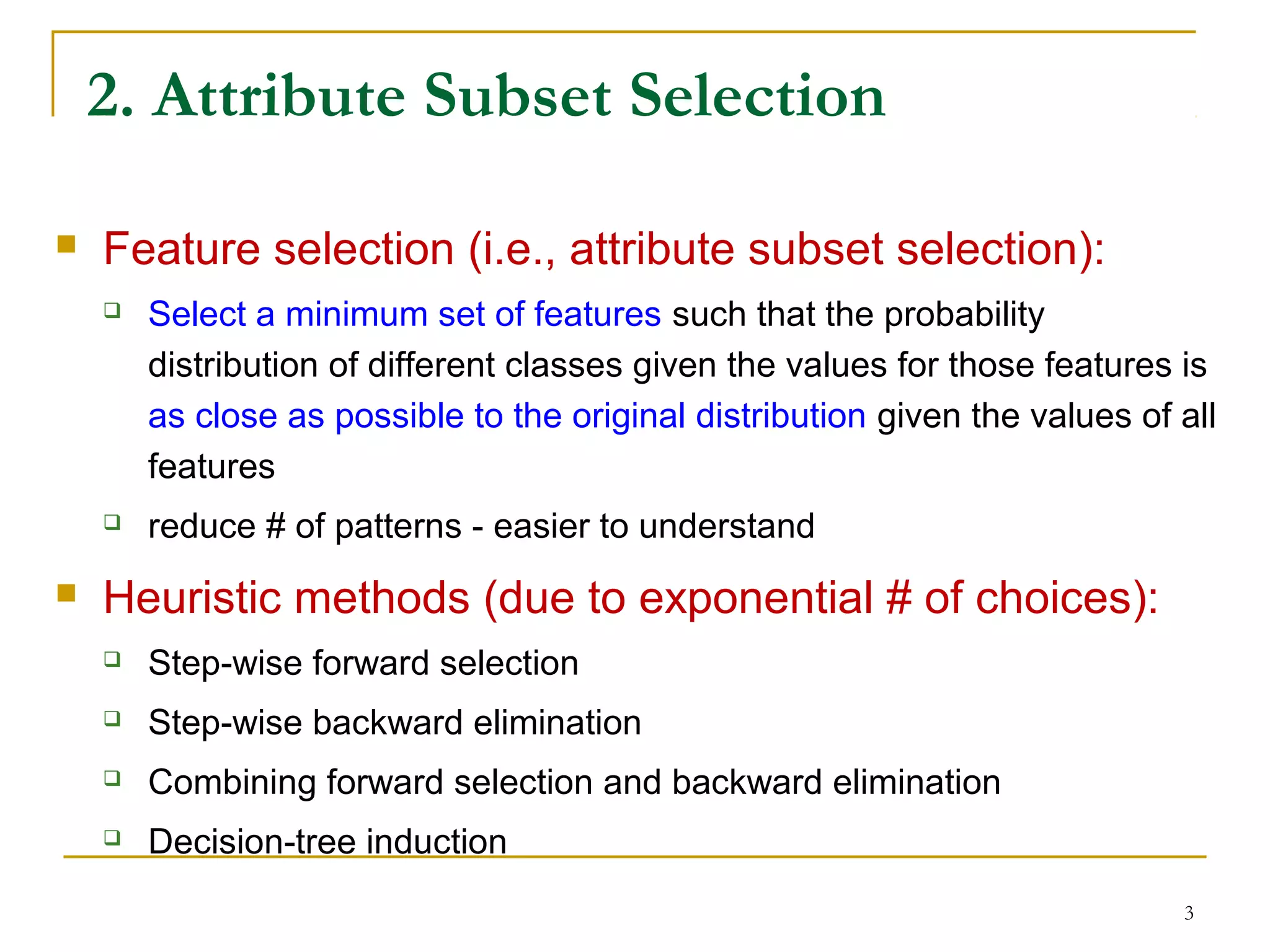
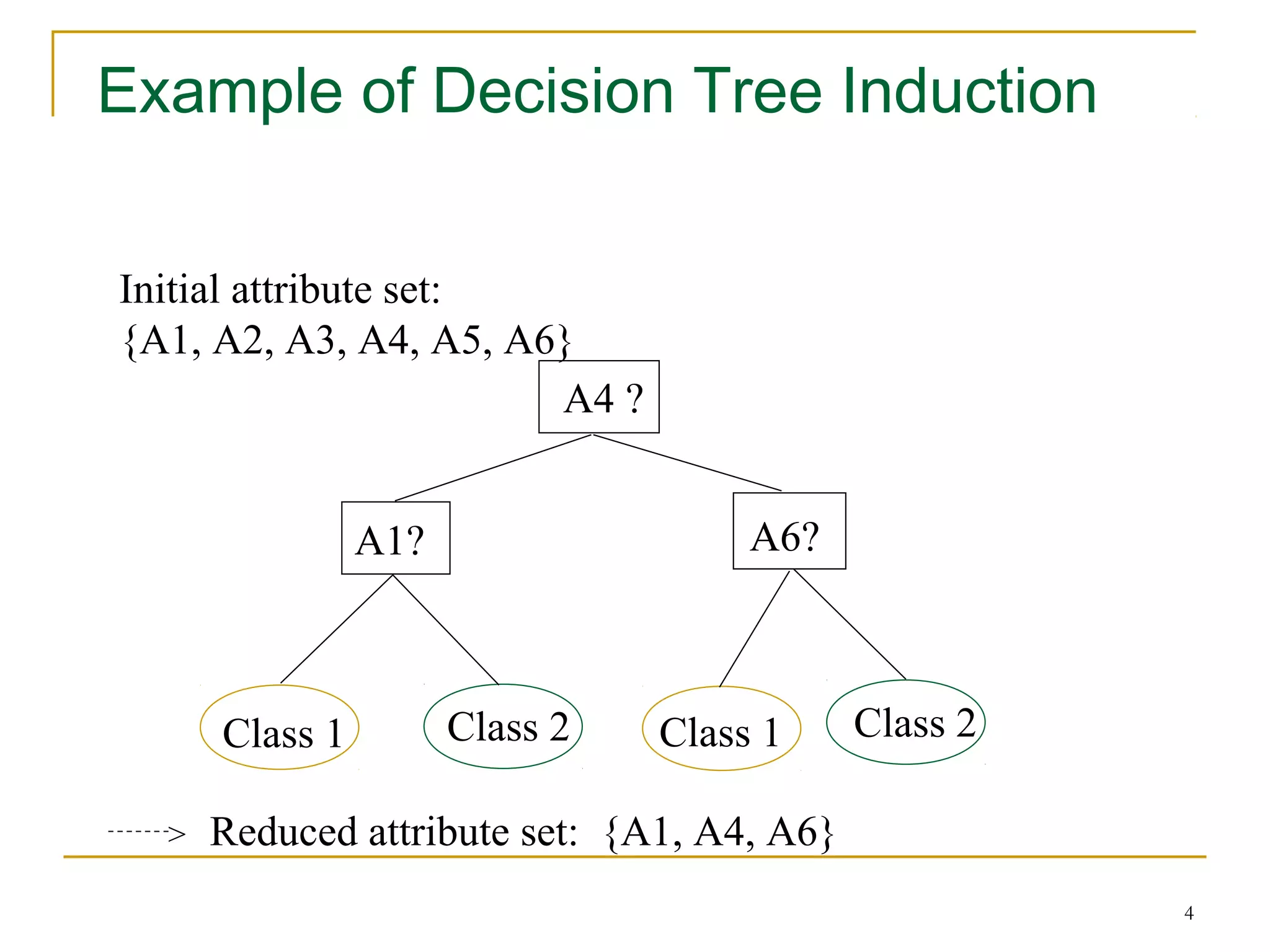
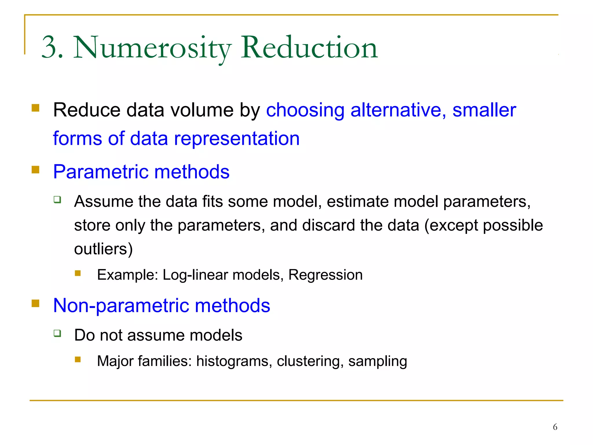
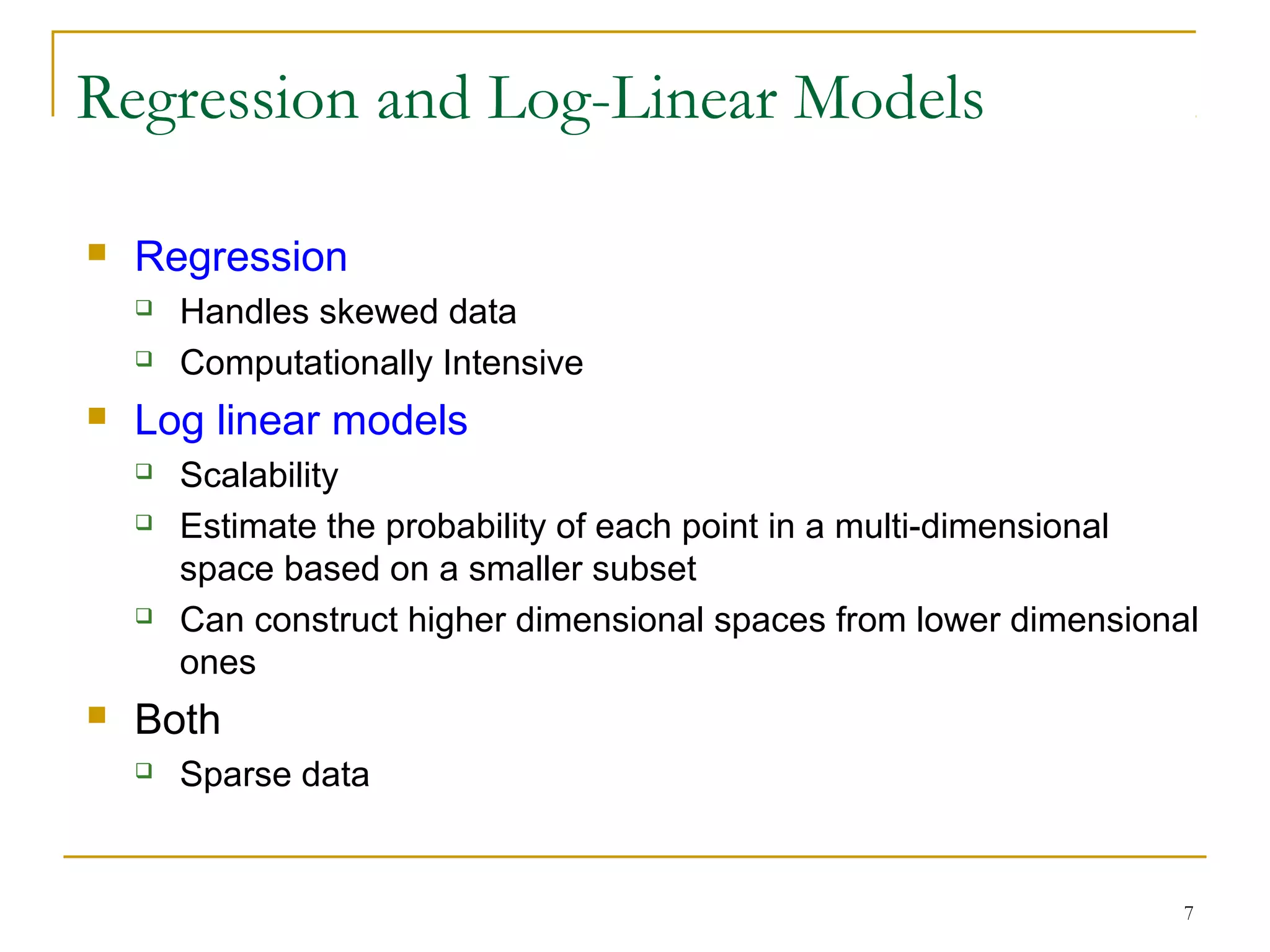
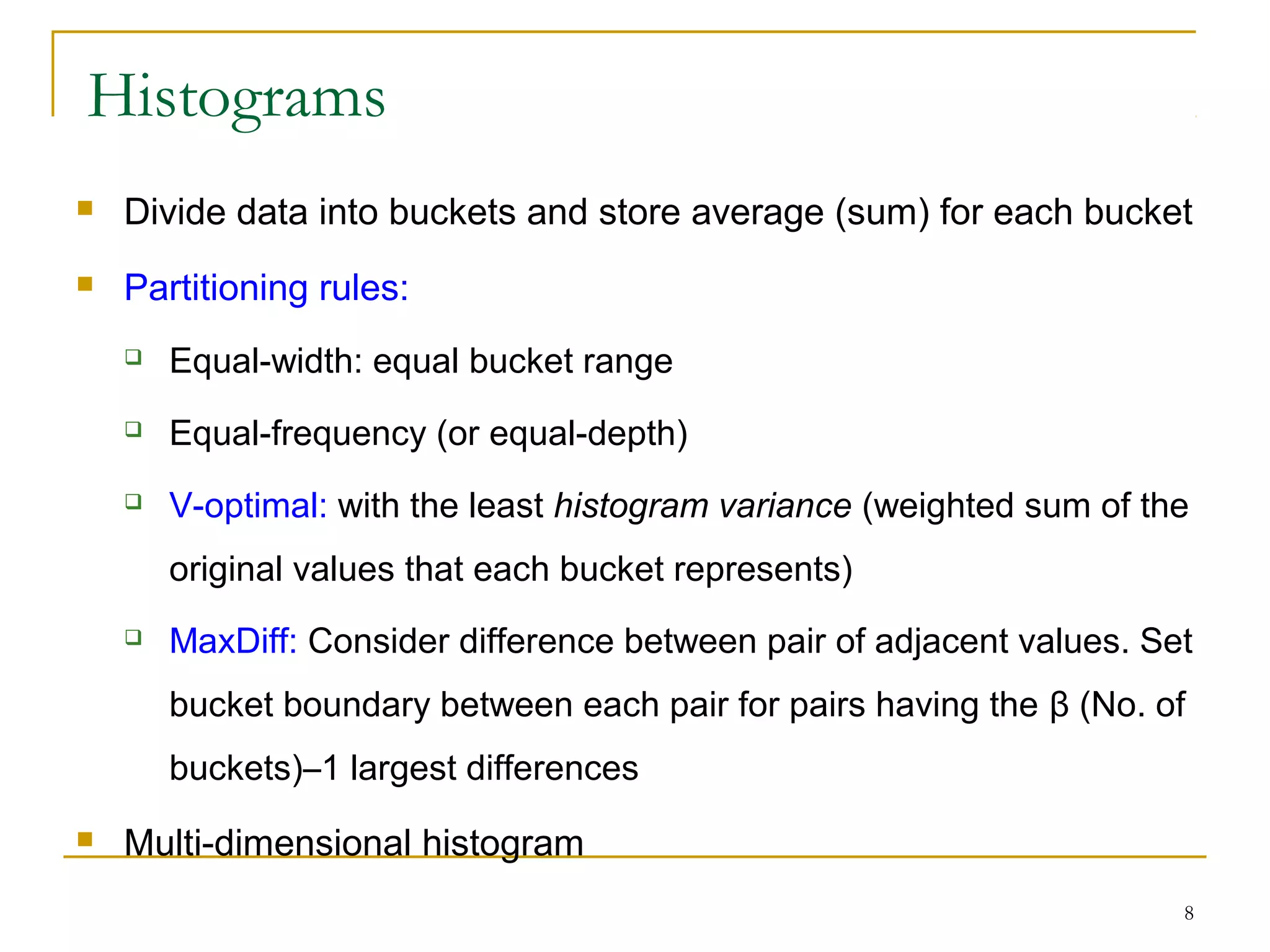
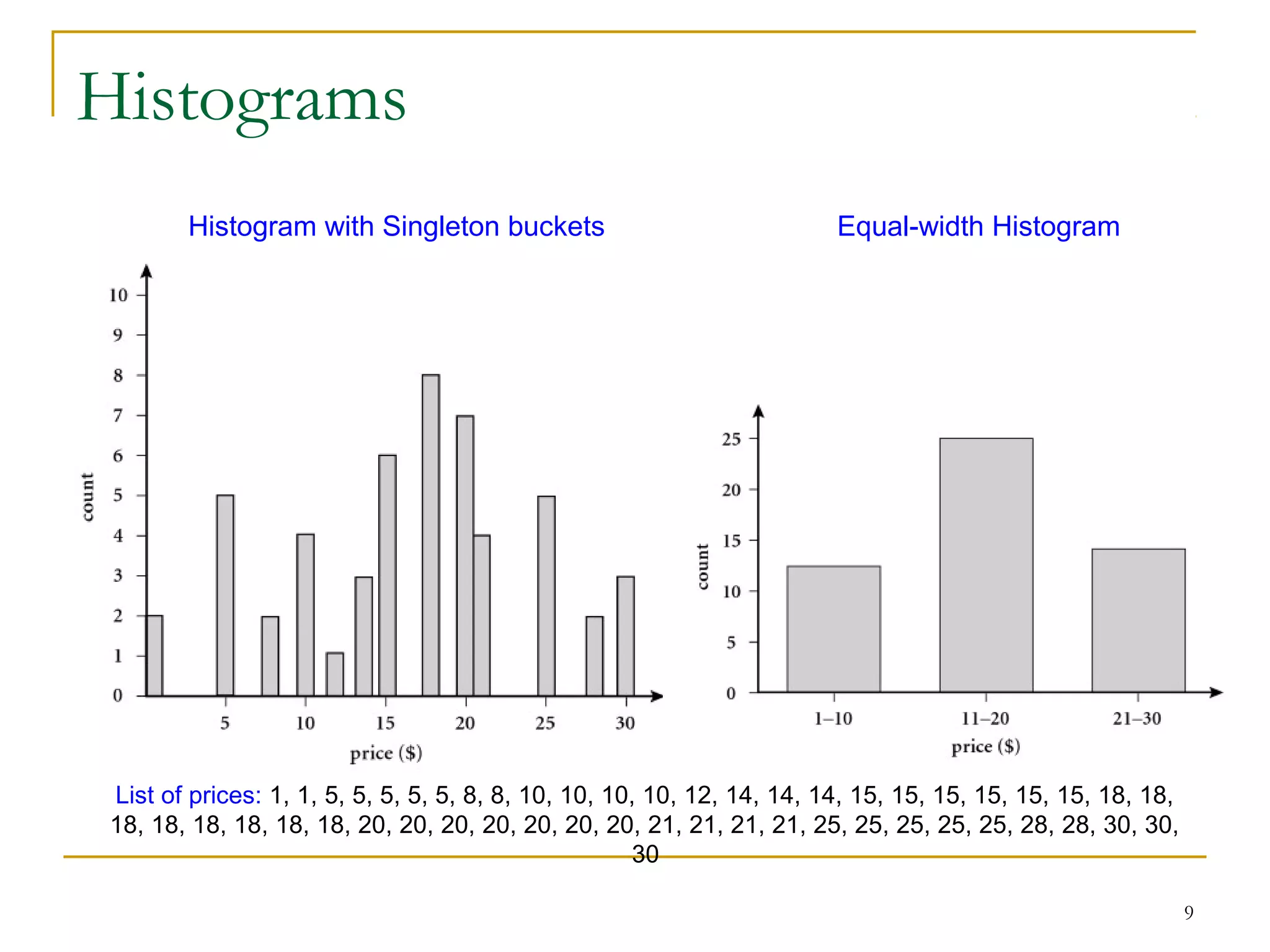
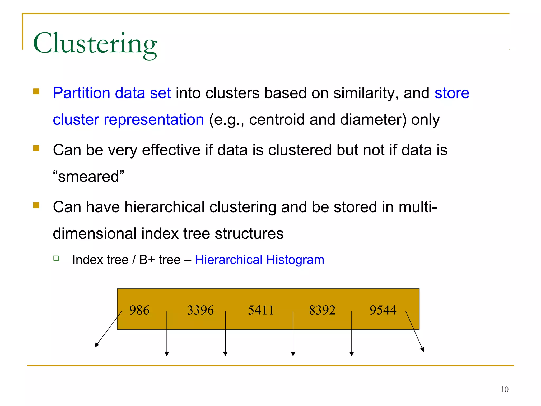
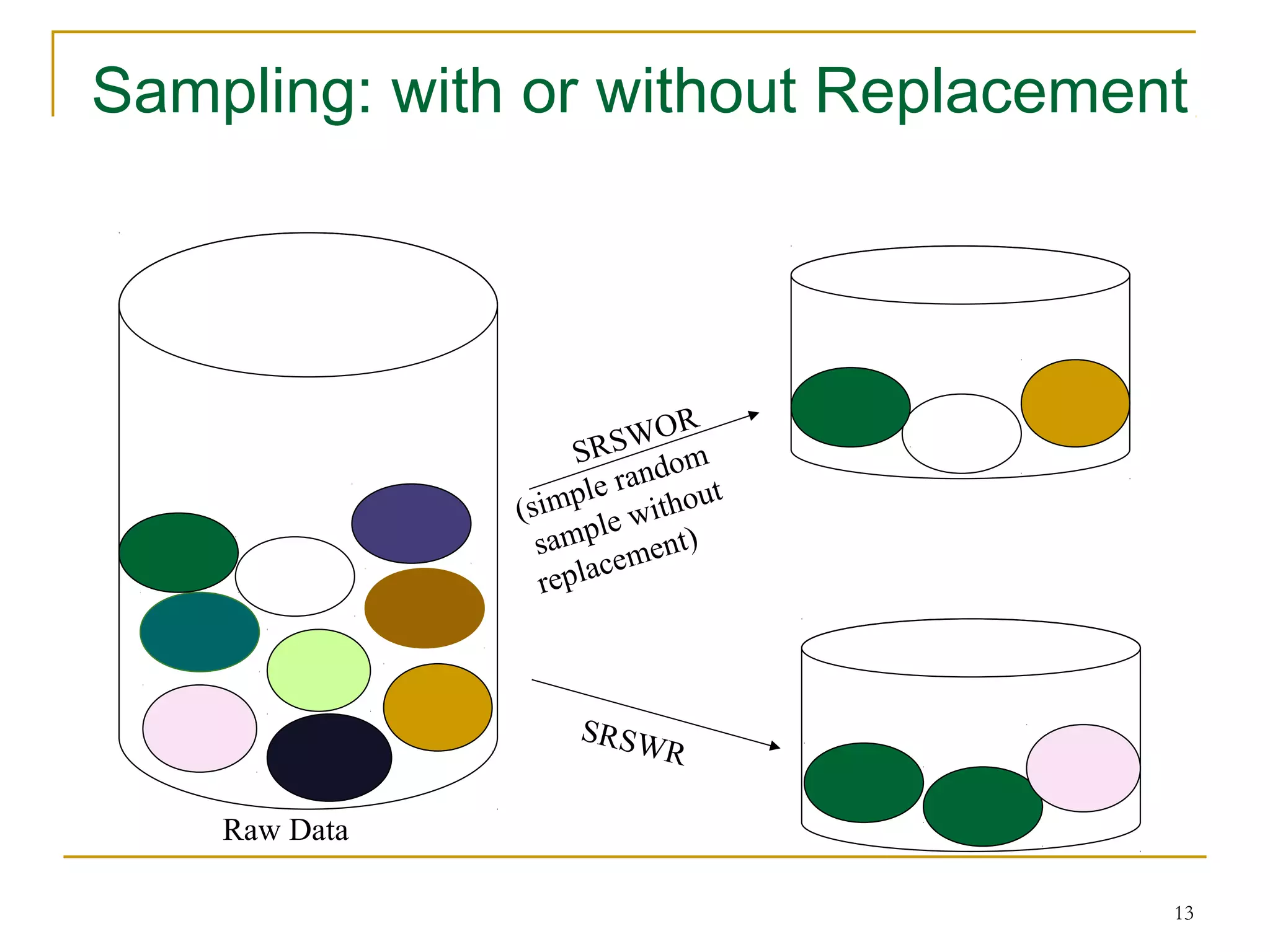
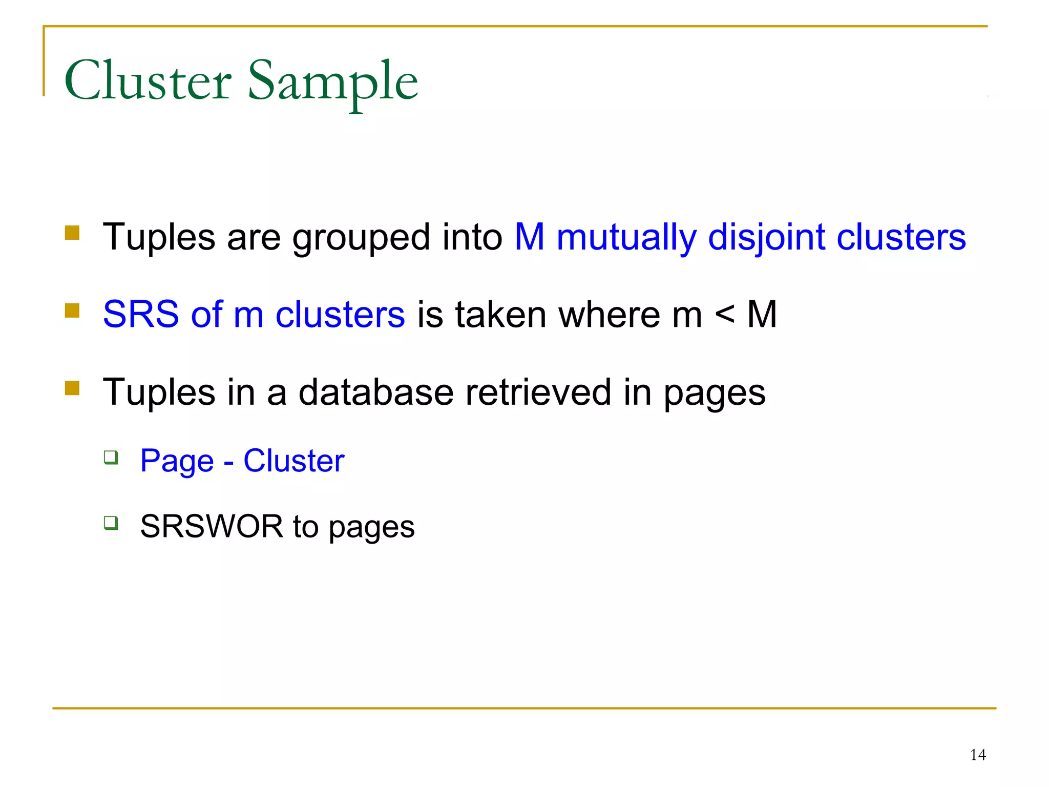
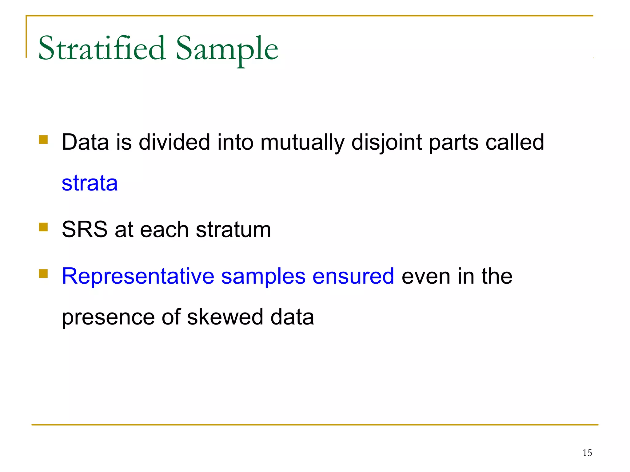
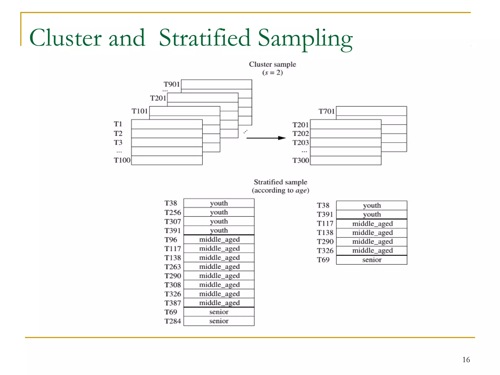
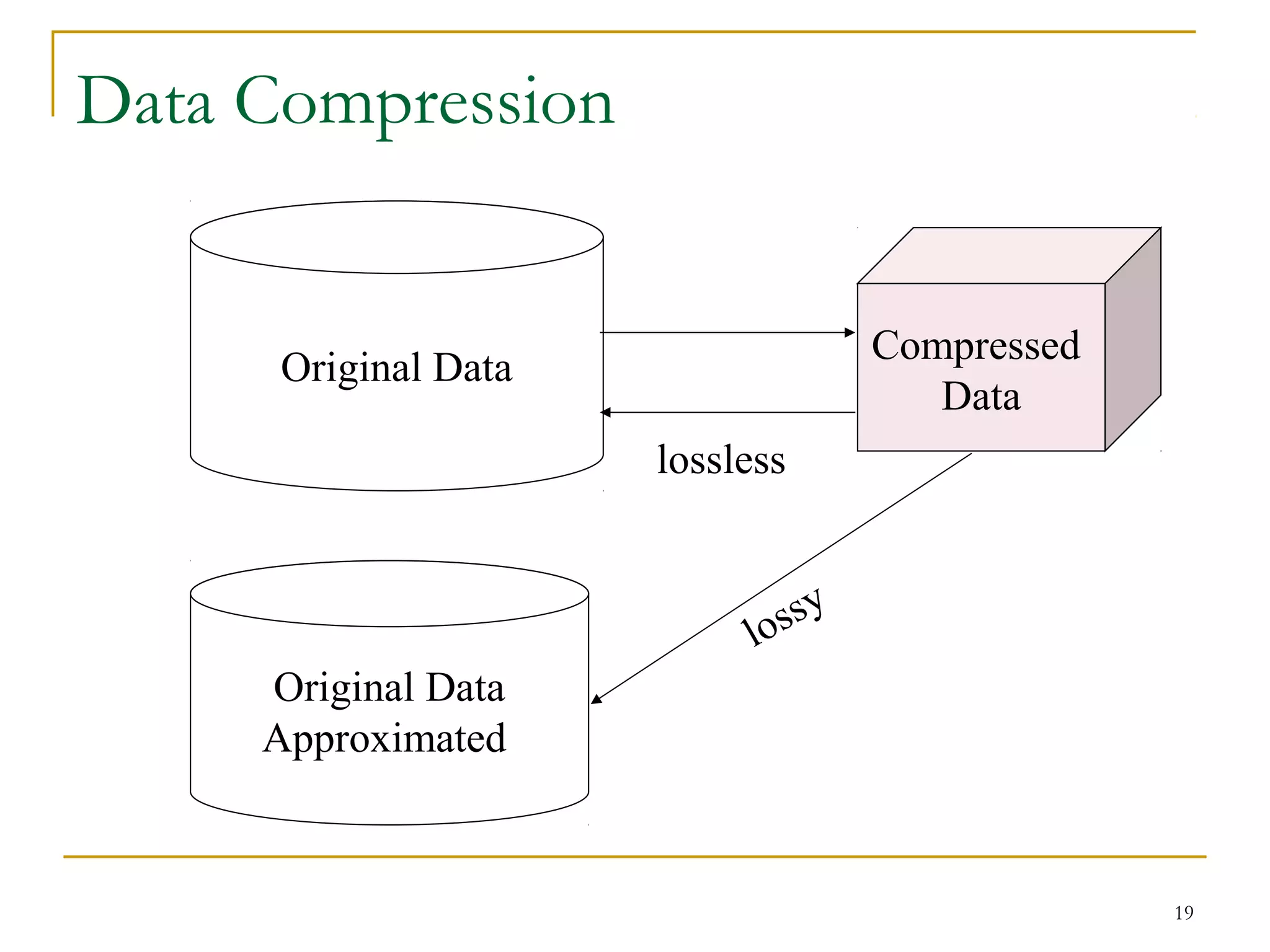
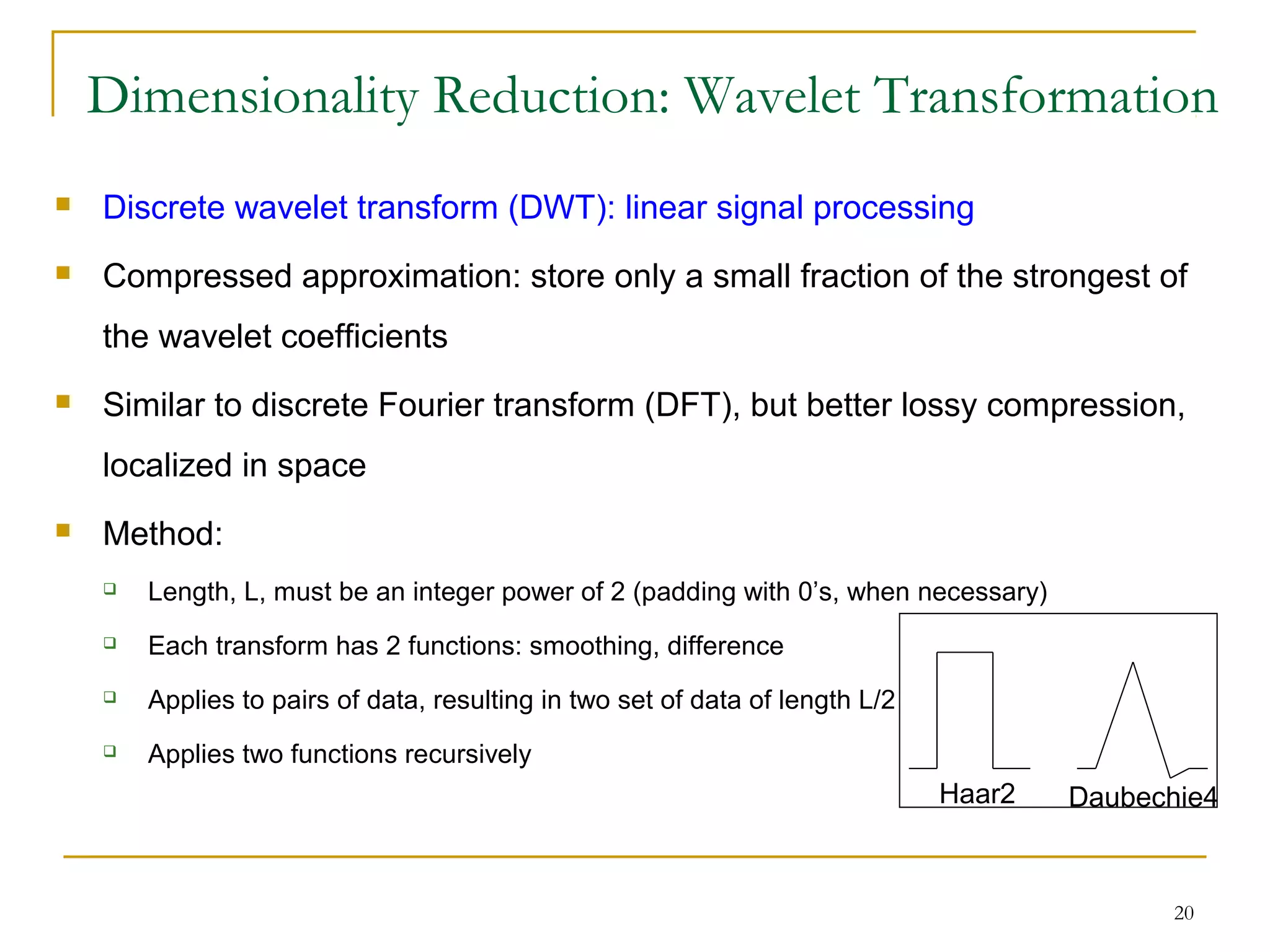
1. 1
Data Reduction

2. 2
Data Reduction Strategies
 Need for data reduction
 A database/data warehouse may store terabytes of data
 Complex data analysis/mining may take a very long time to run on the
complete data set
 Data reduction
 Obtain a reduced representation of the data set that is much smaller in
volume but yet produce the same (or almost the same) analytical results
 Data reduction strategies
 Data cube aggregation
 Attribute Subset Selection
 Numerosity reduction — e.g., fit data into models
 Dimensionality reduction - Data Compression
 Discretization and concept hierarchy generation

3. 3
2. Attribute Subset Selection
 Feature selection (i.e., attribute subset selection):
 Select a minimum set of features such that the probability
distribution of different classes given the values for those features is
as close as possible to the original distribution given the values of all
features
 reduce # of patterns - easier to understand
 Heuristic methods (due to exponential # of choices):
 Step-wise forward selection
 Step-wise backward elimination
 Combining forward selection and backward elimination
 Decision-tree induction

4. 4
Example of Decision Tree Induction
Initial attribute set:
{A1, A2, A3, A4, A5, A6}
A4 ?
A1? A6?
Class 1 Class 2 Class 1 Class 2
> Reduced attribute set: {A1, A4, A6}

5. 5
Heuristic Feature Selection Methods
 There are 2d
possible sub-features of d features
 Several heuristic feature selection methods:
 Best single features under the feature independence assumption:
choose by significance tests
 Best step-wise feature selection
 The best single-feature is picked first
 Then next best feature condition to the first, ...
 Step-wise feature elimination
 Repeatedly eliminate the worst feature
 Best combined feature selection and elimination

6. 6
3. Numerosity Reduction
 Reduce data volume by choosing alternative, smaller
forms of data representation
 Parametric methods
 Assume the data fits some model, estimate model parameters,
store only the parameters, and discard the data (except possible
outliers)
 Example: Log-linear models, Regression
 Non-parametric methods
 Do not assume models
 Major families: histograms, clustering, sampling

7. 7
 Regression
 Handles skewed data
 Computationally Intensive
 Log linear models
 Scalability
 Estimate the probability of each point in a multi-dimensional
space based on a smaller subset
 Can construct higher dimensional spaces from lower dimensional
ones
 Both
 Sparse data
Regression and Log-Linear Models

8. 8
Histograms
 Divide data into buckets and store average (sum) for each bucket
 Partitioning rules:
 Equal-width: equal bucket range
 Equal-frequency (or equal-depth)
 V-optimal: with the least histogram variance (weighted sum of the
original values that each bucket represents)
 MaxDiff: Consider difference between pair of adjacent values. Set
bucket boundary between each pair for pairs having the β (No. of
buckets)–1 largest differences
 Multi-dimensional histogram

9. Histograms
9
List of prices: 1, 1, 5, 5, 5, 5, 5, 8, 8, 10, 10, 10, 10, 12, 14, 14, 14, 15, 15, 15, 15, 15, 15, 18, 18,
18, 18, 18, 18, 18, 18, 20, 20, 20, 20, 20, 20, 20, 21, 21, 21, 21, 25, 25, 25, 25, 25, 28, 28, 30, 30,
30
Histogram with Singleton buckets Equal-width Histogram

10. 10
Clustering
 Partition data set into clusters based on similarity, and store
cluster representation (e.g., centroid and diameter) only
 Can be very effective if data is clustered but not if data is
“smeared”
 Can have hierarchical clustering and be stored in multi-
dimensional index tree structures
 Index tree / B+ tree – Hierarchical Histogram
986 3396 5411 8392 9544

11. 11
Sampling
 Sampling: obtaining a small sample s to represent the whole data
set N
 Allow a mining algorithm to run in complexity that is potentially
sub-linear to the size of the data
 Choose a representative subset of the data
 Simple random sampling may have very poor performance in the
presence of skew
 Develop adaptive sampling methods
 Stratified sampling

12. 12
Sampling Techniques
 Simple Random Sample Without Replacement (SRSWOR)
 Simple Random Sample With Replacement (SRSWR)
 Cluster Sample
 Stratified Sample

13. 13
Sampling: with or without Replacement
SRSWOR
(simple random
sample without
replacement)
SRSWR
Raw Data

14. 14
Cluster Sample
 Tuples are grouped into M mutually disjoint clusters
 SRS of m clusters is taken where m < M
 Tuples in a database retrieved in pages
 Page - Cluster
 SRSWOR to pages

15. 15
Stratified Sample
 Data is divided into mutually disjoint parts called
strata
 SRS at each stratum
 Representative samples ensured even in the
presence of skewed data

16. 16
Cluster and Stratified Sampling
Raw Data

17. 17
Features
 Cost depends on size of sample
 Sub-linear on size of data
 Linear with respect to dimensions
 Estimates answer to an aggregate query

18. 18
Data Compression
 String compression
 There are extensive theories and well-tuned algorithms
 Typically lossless
 But only limited manipulation is possible
 Audio/video compression
 Typically lossy compression, with progressive refinement
 Sometimes small fragments of signal can be reconstructed without
reconstructing the whole

19. 19
Data Compression
Original Data
Compressed
Data
lossless
Original Data
Approximated
lossy

20. 20
Dimensionality Reduction: Wavelet Transformation
 Discrete wavelet transform (DWT): linear signal processing
 Compressed approximation: store only a small fraction of the strongest of
the wavelet coefficients
 Similar to discrete Fourier transform (DFT), but better lossy compression,
localized in space
 Method:
 Length, L, must be an integer power of 2 (padding with 0’s, when necessary)
 Each transform has 2 functions: smoothing, difference
 Applies to pairs of data, resulting in two set of data of length L/2
 Applies two functions recursively
Haar2 Daubechie4

21. 21
Discrete Wavelet Transform
 Can also apply Matrix Multiplication
 Fast DWT algorithm
 Can be applied to Multi-Dimensional data such as Data Cubes
 Wavelet transforms work well on sparse or skewed data
 Used in Computer Vision, Compression of finger print images

22. 22
 Given N data vectors from k-dimensions, find c ≤ k orthogonal vectors
(Principal components) that can be best used to represent data
 Steps
 Normalize input data: Each attribute falls within the same range
 Compute c orthonormal (unit) vectors, i.e., principal components
 Each input data (vector) is a linear combination of the c principal component
vectors
 The principal components are sorted in order of decreasing “significance” or
strength
 Since the components are sorted, the size of the data can be reduced by
eliminating the weak components, i.e., those with low variance. (i.e., using the
strongest principal components, it is possible to reconstruct a good
approximation of the original data)
 Works for numeric data only
 Used for handling sparse data
Dimensionality Reduction: Principal
Component Analysis (PCA)

23. 23
X1
X2
Y1
Y2
Principal Component Analysis