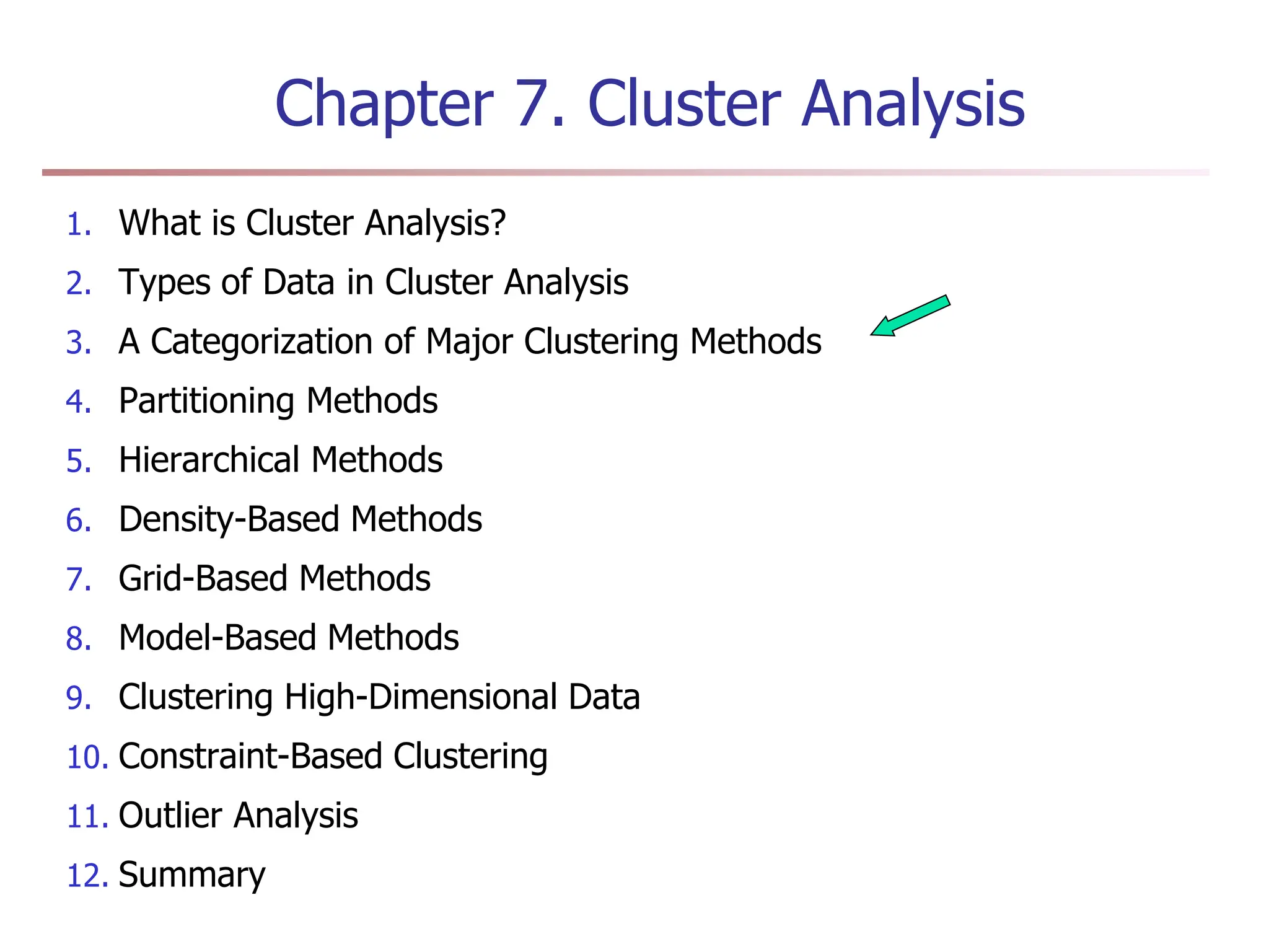
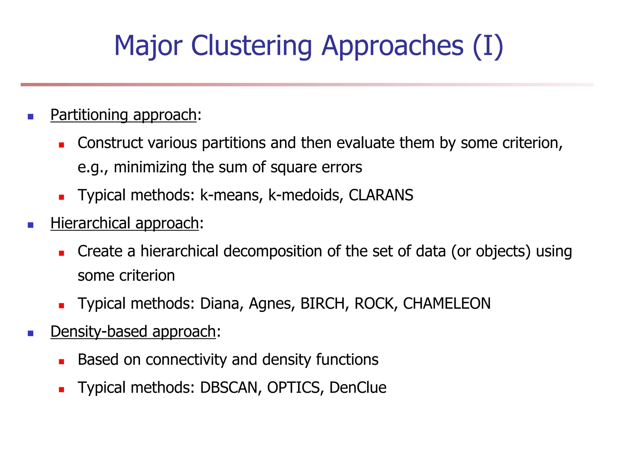
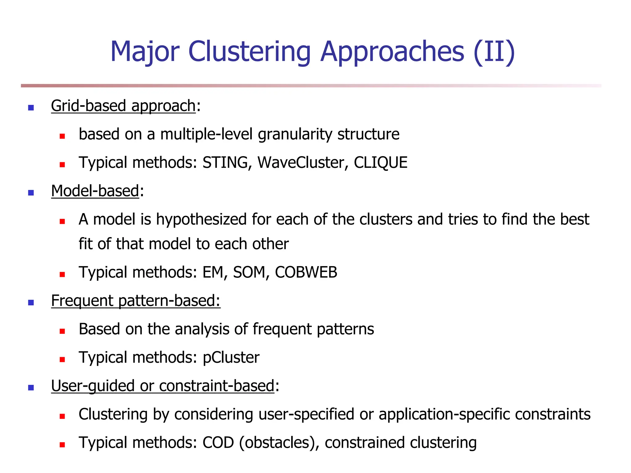
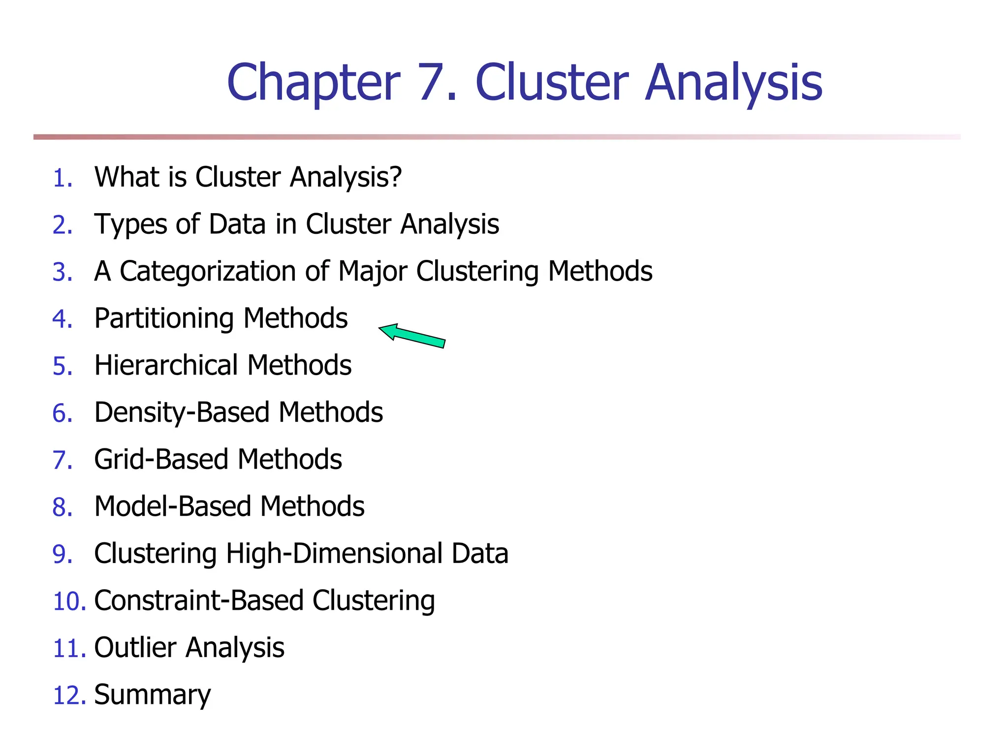
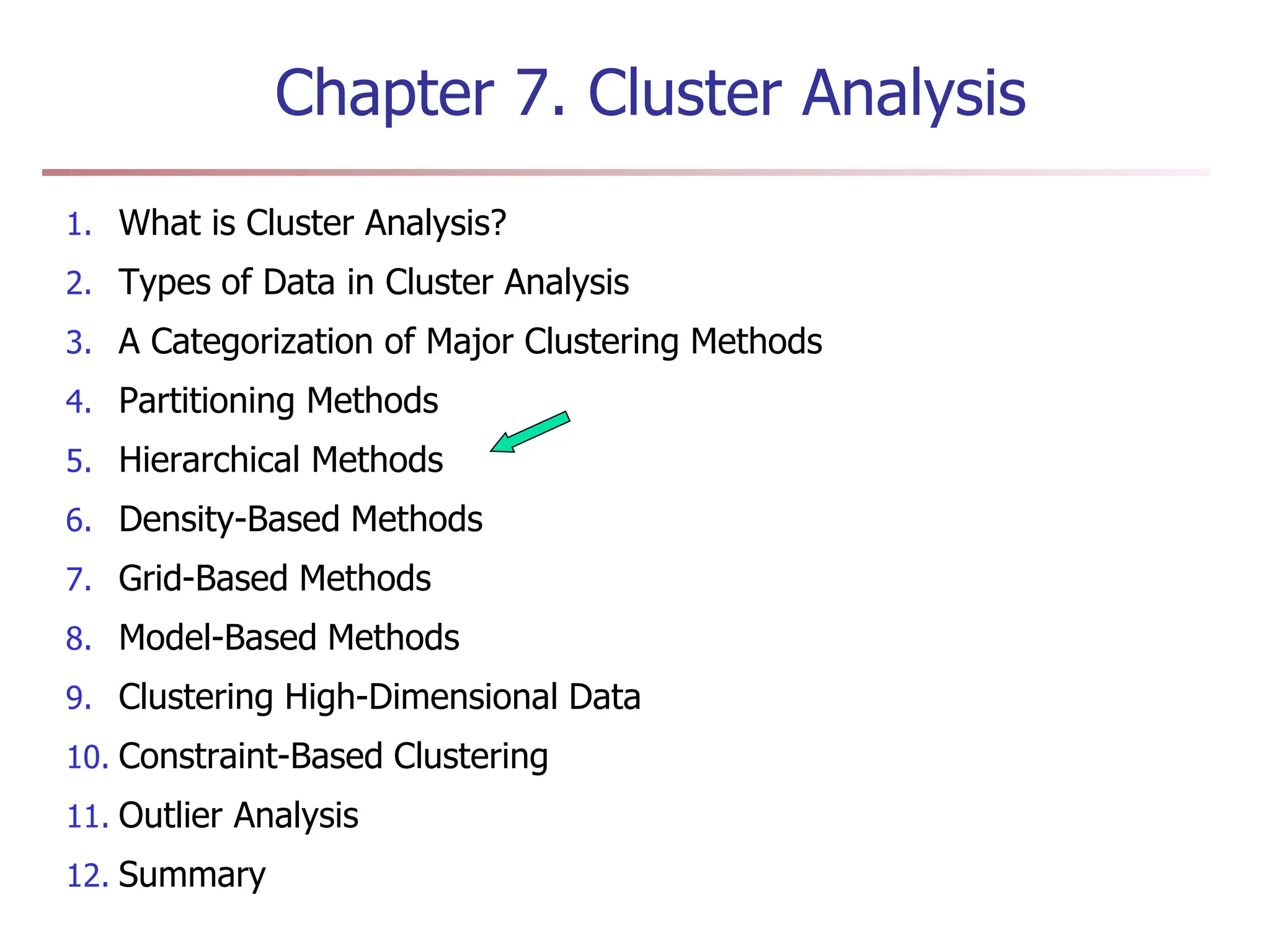
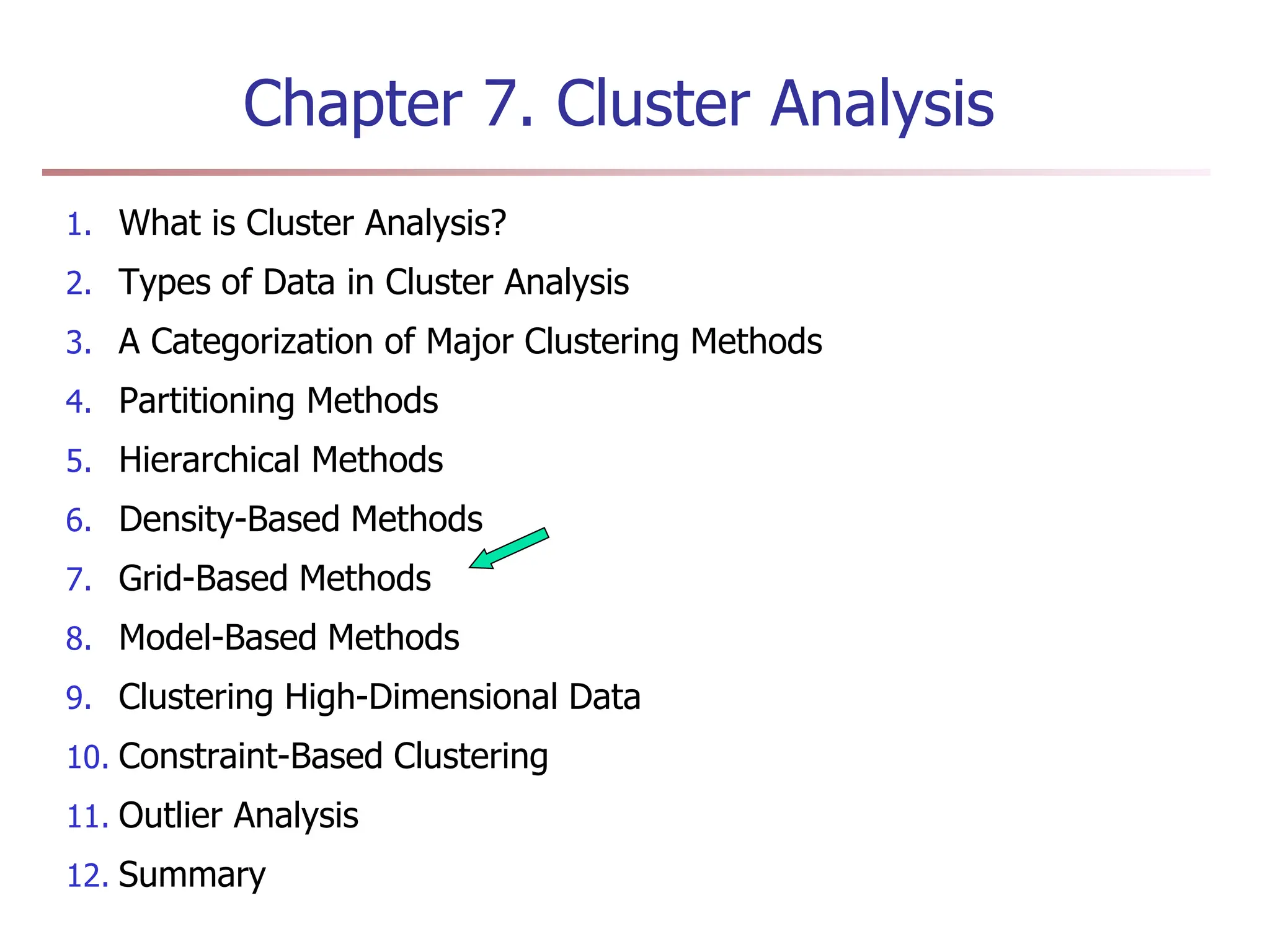
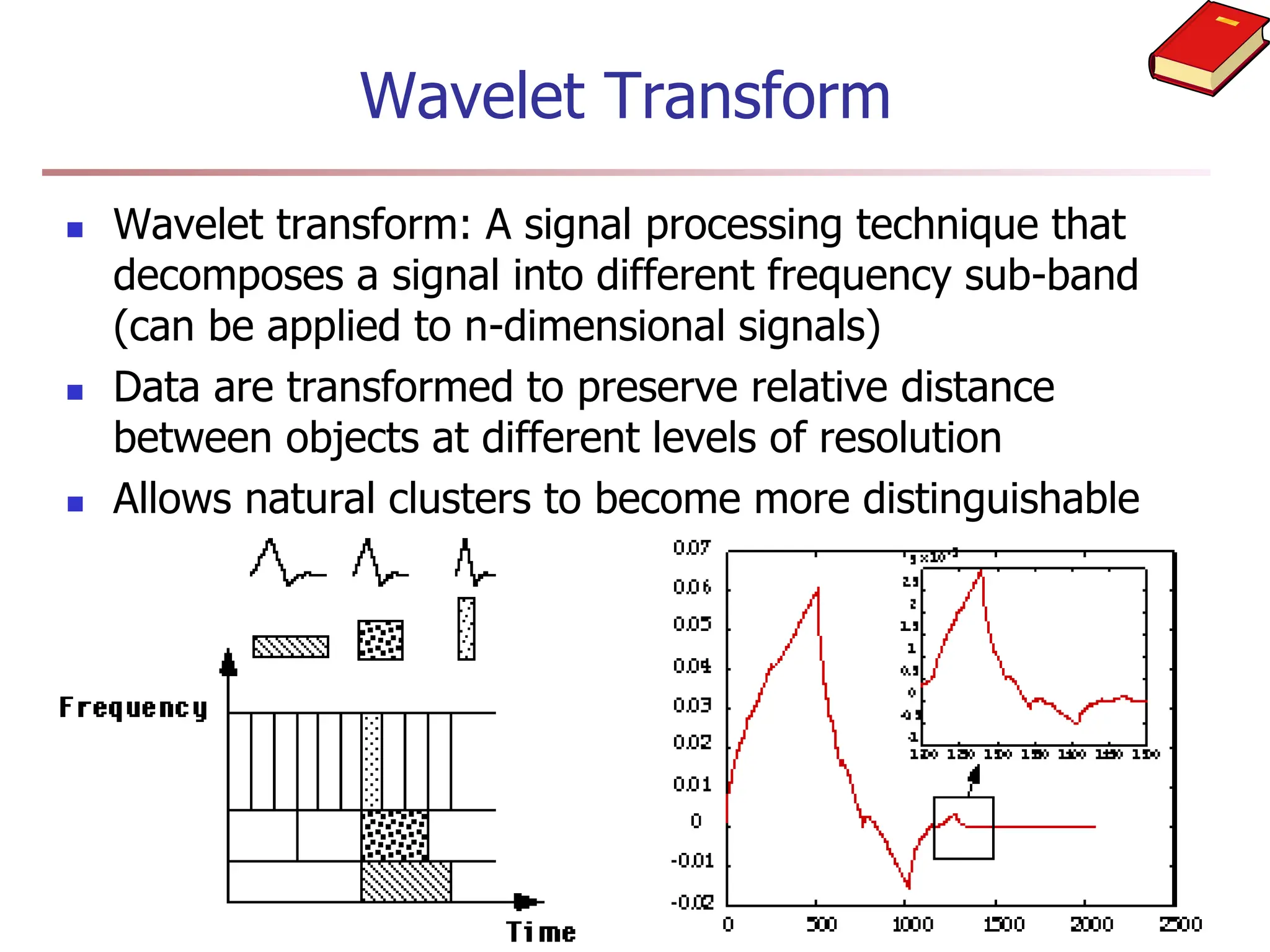
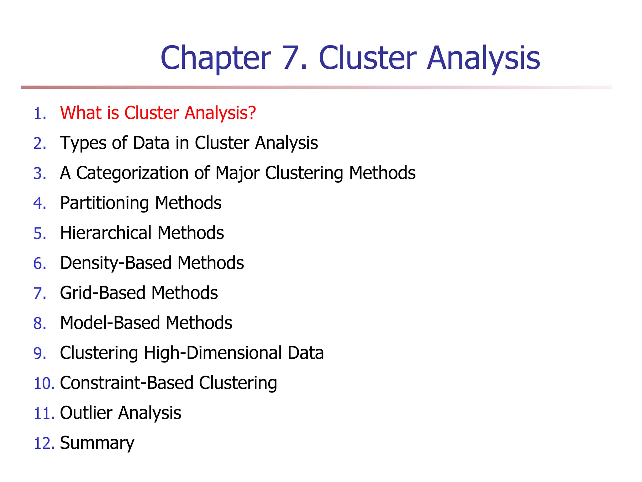
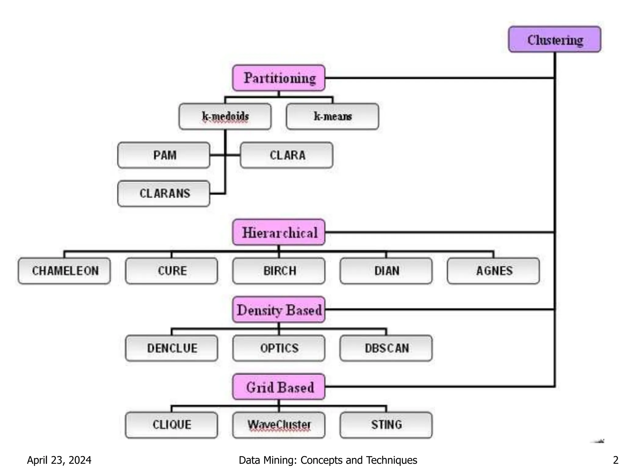
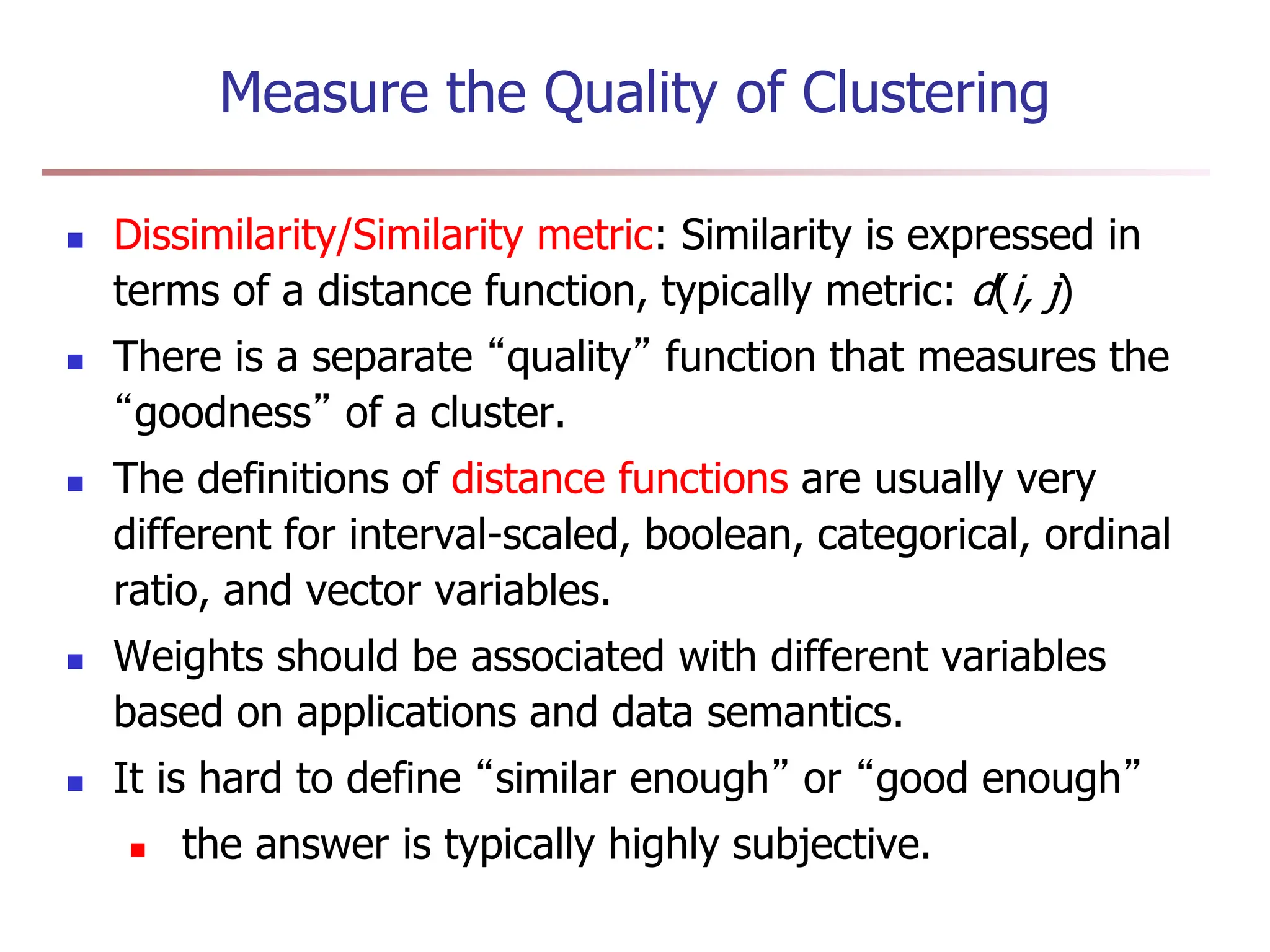
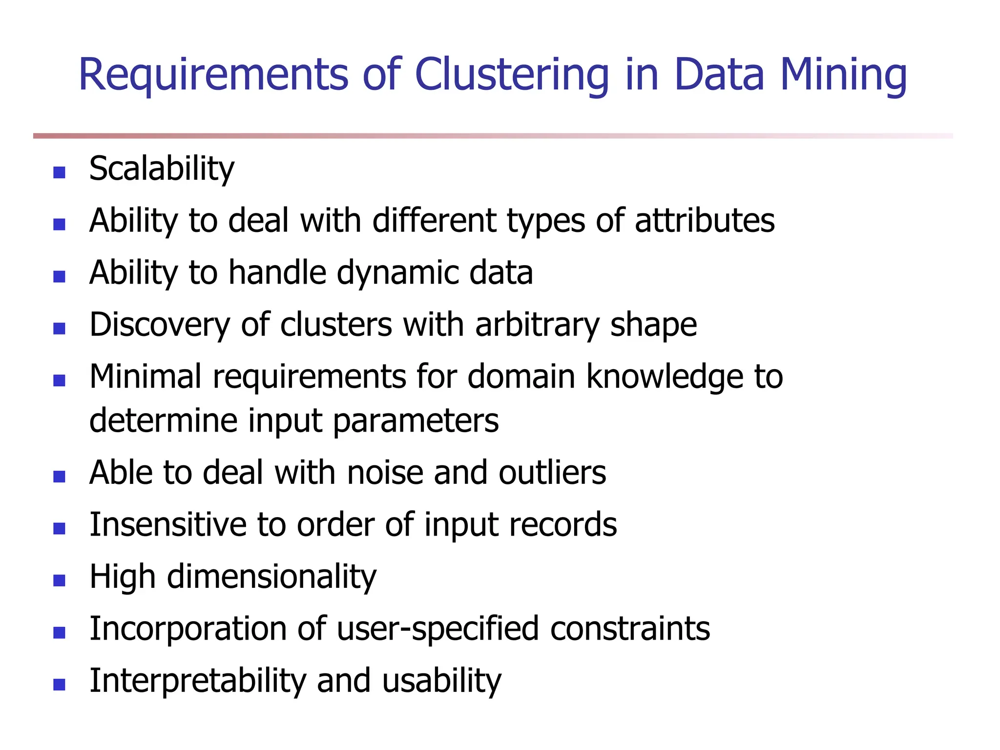
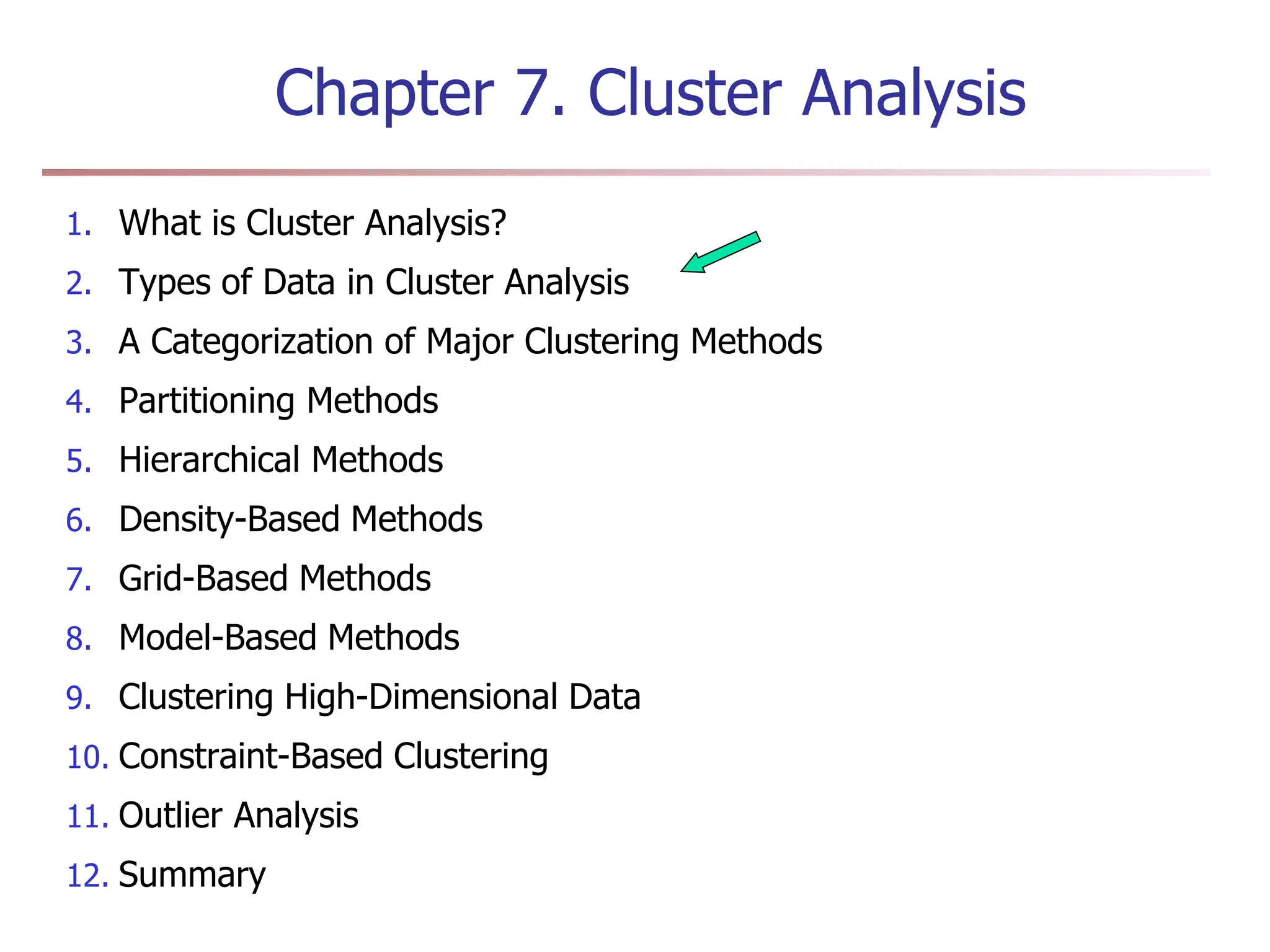
SlideShare a Scribd company logo
1 of 123
Chapter 7. Cluster Analysis
1. What is Cluster Analysis?
2. Types of Data in Cluster Analysis
3. A Categorization of Major Clustering Methods
4. Partitioning Methods
5. Hierarchical Methods
6. Density-Based Methods
7. Grid-Based Methods
8. Model-Based Methods
9. Clustering High-Dimensional Data
10. Constraint-Based Clustering
11. Outlier Analysis
12. Summary
April 23, 2024 Data Mining: Concepts and Techniques 2
What is Cluster Analysis?
 Cluster: a collection of data objects
 Similar to one another within the same cluster
 Dissimilar to the objects in other clusters
 Cluster analysis
 Finding similarities between data according to the
characteristics found in the data and grouping similar
data objects into clusters
 Unsupervised learning: no predefined classes
 Typical applications
 As a stand-alone tool to get insight into data distribution
 As a preprocessing step for other algorithms
Clustering: Rich Applications and
Multidisciplinary Efforts
 Pattern Recognition
 Spatial Data Analysis
 Create thematic maps in GIS by clustering feature
spaces
 Detect spatial clusters or for other spatial mining tasks
 Image Processing
 Economic Science (especially market research)
 WWW
 Document classification
 Cluster Weblog data to discover groups of similar access
patterns
Examples of Clustering Applications
 Marketing: Help marketers discover distinct groups in their customer
bases, and then use this knowledge to develop targeted marketing
programs
 Land use: Identification of areas of similar land use in an earth
observation database
 Insurance: Identifying groups of motor insurance policy holders with
a high average claim cost
 City-planning: Identifying groups of houses according to their house
type, value, and geographical location
 Earth-quake studies: Observed earth quake epicenters should be
clustered along continent faults
Quality: What Is Good Clustering?
 A good clustering method will produce high quality
clusters with
 high intra-class similarity
 low inter-class similarity
 The quality of a clustering result depends on both the
similarity measure used by the method and its
implementation
 The quality of a clustering method is also measured by its
ability to discover some or all of the hidden patterns
Measure the Quality of Clustering
 Dissimilarity/Similarity metric: Similarity is expressed in
terms of a distance function, typically metric: d(i, j)
 There is a separate “quality” function that measures the
“goodness” of a cluster.
 The definitions of distance functions are usually very
different for interval-scaled, boolean, categorical, ordinal
ratio, and vector variables.
 Weights should be associated with different variables
based on applications and data semantics.
 It is hard to define “similar enough” or “good enough”
 the answer is typically highly subjective.
Requirements of Clustering in Data Mining
 Scalability
 Ability to deal with different types of attributes
 Ability to handle dynamic data
 Discovery of clusters with arbitrary shape
 Minimal requirements for domain knowledge to
determine input parameters
 Able to deal with noise and outliers
 Insensitive to order of input records
 High dimensionality
 Incorporation of user-specified constraints
 Interpretability and usability
Chapter 7. Cluster Analysis
1. What is Cluster Analysis?
2. Types of Data in Cluster Analysis
3. A Categorization of Major Clustering Methods
4. Partitioning Methods
5. Hierarchical Methods
6. Density-Based Methods
7. Grid-Based Methods
8. Model-Based Methods
9. Clustering High-Dimensional Data
10. Constraint-Based Clustering
11. Outlier Analysis
12. Summary
Data Structures
 Data matrix
 n x p
 object-by-variable
 Dissimilarity matrix
 n x n
 object-by-object


















np
x
...
nf
x
...
n1
x
...
...
...
...
...
ip
x
...
if
x
...
i1
x
...
...
...
...
...
1p
x
...
1f
x
...
11
x
















0
...
)
2
,
(
)
1
,
(
:
:
:
)
2
,
3
(
)
...
n
d
n
d
0
d
d(3,1
0
d(2,1)
0
Type of data in clustering analysis
 Interval-scaled variables
 Binary variables
 Nominal, ordinal, and ratio variables
 Variables of mixed types
Interval-scaled variables
 Standardize data
 Calculate the mean absolute deviation:
where
 Calculate the standardized measurement (z-score)
 Using mean absolute deviation is more robust than using
standard deviation
.
)
...
2
1
1
nf
f
f
f
x
x
(x
n
m 



|)
|
...
|
|
|
(|
1
2
1 f
nf
f
f
f
f
f
m
x
m
x
m
x
n
s 






f
f
if
if s
m
x
z


Similarity and Dissimilarity Between
Objects
 Distances are normally used to measure the similarity or
dissimilarity between two data objects
 Some popular ones include: Minkowski distance:
where i = (xi1, xi2, …, xip) and j = (xj1, xj2, …, xjp) are
two p-dimensional data objects, and q is a positive
integer
 If q = 1, d is Manhattan distance
q
q
p
p
q
q
j
x
i
x
j
x
i
x
j
x
i
x
j
i
d )
|
|
...
|
|
|
(|
)
,
(
2
2
1
1







|
|
...
|
|
|
|
)
,
(
2
2
1
1 p
p j
x
i
x
j
x
i
x
j
x
i
x
j
i
d 






Similarity and Dissimilarity Between
Objects (Cont.)
 If q = 2, d is Euclidean distance:
 Properties
 d(i,j)  0
 d(i,i) = 0
 d(i,j) = d(j,i)
 d(i,j)  d(i,k) + d(k,j)
 Also, one can use weighted distance, parametric
Pearson product moment correlation, or other
disimilarity measures
)
|
|
...
|
|
|
(|
)
,
( 2
2
2
2
2
1
1 p
p j
x
i
x
j
x
i
x
j
x
i
x
j
i
d 






Binary Variables
 A contingency table for binary
data
 Distance measure for
symmetric binary variables:
 Distance measure for
asymmetric binary variables:
 Jaccard coefficient (similarity
measure for asymmetric
binary variables):
d
c
b
a
c
b
j
i
d





)
,
(
c
b
a
c
b
j
i
d




)
,
(
p
d
b
c
a
sum
d
c
d
c
b
a
b
a
sum




0
1
0
1
Object i
Object j
c
b
a
a
j
i
simJaccard



)
,
(
Dissimilarity between Binary Variables
 Example
 gender is a symmetric attribute
 the remaining attributes are asymmetric binary
 let the values Y and P be set to 1, and the value N be set to 0
 Suppose distance is computed based on the asymmetric variables
Name Gender Fever Cough Test-1 Test-2 Test-3 Test-4
Jack M Y N P N N N
Mary F Y N P N P N
Jim M Y P N N N N
75
.
0
2
1
1
2
1
)
,
(
67
.
0
1
1
1
1
1
)
,
(
33
.
0
1
0
2
1
0
)
,
(















mary
jim
d
jim
jack
d
mary
jack
d
Categorical Variables
 A generalization of the binary variable in that it can take
more than 2 states, e.g., red, yellow, blue, green
 Method 1 (sym.): Simple matching
 m: # of matches, p: total # of variables
 Method 2 (asym.): use a large number of binary variables
 creating a new binary variable for each of the M nominal
states
p
m
p
j
i
d 

)
,
(
Ordinal Variables
 An ordinal variable can be discrete or continuous
 Order is important, e.g., rank
 Can be treated like interval-scaled
 replace xif by their rank
 map the range of each variable onto [0, 1] by replacing
i-th object in the f-th variable by
 compute the dissimilarity using methods for interval-
scaled variables
1
1



f
if
if M
r
z
}
,...,
1
{ f
if
M
r 
Ratio-Scaled Variables
 Ratio-scaled variable: a positive measurement on a
nonlinear scale, approximately at exponential scale,
such as AeBt or Ae-Bt
 Methods:
 treat them like interval-scaled variables—not a good
choice! (why?—the scale can be distorted)
 apply logarithmic transformation
yif = log(xif)
 treat them as continuous ordinal data treat their rank
as interval-scaled
Variables of Mixed Types
 A database may contain all the six types of variables
 symmetric binary, asymmetric binary, nominal,
ordinal, interval and ratio
 One may use a weighted formula to combine their
effects
 f is binary or nominal:
dij
(f) = 0 if xif = xjf , or dij
(f) = 1 otherwise
 f is interval-based: use the normalized distance
 f is ordinal or ratio-scaled
 compute ranks rif and
 and treat zif as interval-scaled
)
(
1
)
(
)
(
1
)
,
( f
ij
p
f
f
ij
f
ij
p
f
d
j
i
d







1
1



f
if
M
r
zif
Vector Objects
 Vector objects: keywords in documents, gene
features in micro-arrays, etc.
 Broad applications: information retrieval, biologic
taxonomy, etc.
 Cosine measure: cos() =
 A variant: Tanimoto coefficient
Chapter 7. Cluster Analysis
1. What is Cluster Analysis?
2. Types of Data in Cluster Analysis
3. A Categorization of Major Clustering Methods
4. Partitioning Methods
5. Hierarchical Methods
6. Density-Based Methods
7. Grid-Based Methods
8. Model-Based Methods
9. Clustering High-Dimensional Data
10. Constraint-Based Clustering
11. Outlier Analysis
12. Summary
Major Clustering Approaches (I)
 Partitioning approach:
 Construct various partitions and then evaluate them by some criterion,
e.g., minimizing the sum of square errors
 Typical methods: k-means, k-medoids, CLARANS
 Hierarchical approach:
 Create a hierarchical decomposition of the set of data (or objects) using
some criterion
 Typical methods: Diana, Agnes, BIRCH, ROCK, CHAMELEON
 Density-based approach:
 Based on connectivity and density functions
 Typical methods: DBSCAN, OPTICS, DenClue
Major Clustering Approaches (II)
 Grid-based approach:
 based on a multiple-level granularity structure
 Typical methods: STING, WaveCluster, CLIQUE
 Model-based:
 A model is hypothesized for each of the clusters and tries to find the best
fit of that model to each other
 Typical methods: EM, SOM, COBWEB
 Frequent pattern-based:
 Based on the analysis of frequent patterns
 Typical methods: pCluster
 User-guided or constraint-based:
 Clustering by considering user-specified or application-specific constraints
 Typical methods: COD (obstacles), constrained clustering
Typical Alternatives to Calculate the Distance
between Clusters
 Single link: smallest distance between an element in one cluster
and an element in the other, i.e., dis(Ki, Kj) = min(tip, tjq)
 Complete link: largest distance between an element in one cluster
and an element in the other, i.e., dis(Ki, Kj) = max(tip, tjq)
 Average: avg distance between an element in one cluster and an
element in the other, i.e., dis(Ki, Kj) = avg(tip, tjq)
 Centroid: distance between the centroids of two clusters, i.e.,
dis(Ki, Kj) = dis(Ci, Cj)
 Medoid: distance between the medoids of two clusters, i.e., dis(Ki,
Kj) = dis(Mi, Mj)
 Medoid: one chosen, centrally located object in the cluster
Centroid, Radius and Diameter of a
Cluster (for numerical data sets)
 Centroid: the “middle” of a cluster
 Radius: square root of average distance from any point of the
cluster to its centroid
 Diameter: square root of average mean squared distance between
all pairs of points in the cluster
N
t
N
i ip
m
C
)
(
1



N
m
c
ip
t
N
i
m
R
2
)
(
1




)
1
(
2
)
(
1
1







N
N
iq
t
ip
t
N
i
N
i
m
D
Chapter 7. Cluster Analysis
1. What is Cluster Analysis?
2. Types of Data in Cluster Analysis
3. A Categorization of Major Clustering Methods
4. Partitioning Methods
5. Hierarchical Methods
6. Density-Based Methods
7. Grid-Based Methods
8. Model-Based Methods
9. Clustering High-Dimensional Data
10. Constraint-Based Clustering
11. Outlier Analysis
12. Summary
Partitioning Algorithms: Basic Concept
 Partitioning method: Construct a partition of a database D of n objects
into a set of k clusters, s.t., some objective is minimized. E.g., min
sum of squared distance in k-means
 Given a k, find a partition of k clusters that optimizes the chosen
partitioning criterion
 Global optimal: exhaustively enumerate all partitions
 Heuristic methods: k-means and k-medoids algorithms
 k-means (MacQueen’67): Each cluster is represented by the center
of the cluster
 k-medoids or PAM (Partition around medoids) (Kaufman &
Rousseeuw’87): Each cluster is represented by one of the objects
in the cluster
2
1 )
( mi
m
Km
t
k
m t
C
mi


 

The K-Means Clustering Method
 Given k, the k-means algorithm is implemented in
four steps:
 Partition objects into k nonempty subsets
 Compute seed points as the centroids of the
clusters of the current partition (the centroid is the
center, i.e., mean point, of the cluster)
 Assign each object to the cluster with the nearest
seed point
 Go back to Step 2, stop when no more new
assignment
The K-Means Clustering Method
 Example
0
1
2
3
4
5
6
7
8
9
10
0 1 2 3 4 5 6 7 8 9 10
0
1
2
3
4
5
6
7
8
9
10
0 1 2 3 4 5 6 7 8 9 10
0
1
2
3
4
5
6
7
8
9
10
0 1 2 3 4 5 6 7 8 9 10
0
1
2
3
4
5
6
7
8
9
10
0 1 2 3 4 5 6 7 8 9 10
0
1
2
3
4
5
6
7
8
9
10
0 1 2 3 4 5 6 7 8 9 10
K=2
Arbitrarily choose K
initial cluster centers
(can use k objects)
Assign
each
objects
to most
similar
center
Update
the
cluster
means
Update
the
cluster
means
reassign
reassign
Comments on the K-Means Method
 Strength: Relatively efficient: O(tkn), where n is # objects, k is #
clusters, and t is # iterations. Normally, k, t << n.
 Comparing: PAM: O(k(n-k)2 ), CLARA: O(ks2 + k(n-k))
 Comment: Often terminates at a local optimum. The global optimum
may be found using techniques such as: deterministic annealing and
genetic algorithms
 Weakness
 Applicable only when mean is defined, then what about categorical
data?
 Need to specify k, the number of clusters, in advance
 Unable to handle noisy data and outliers
 Not suitable to discover clusters with non-convex shapes
Variations of the K-Means Method
 A few variants of the k-means which differ in
 Selection of the initial k means
 Dissimilarity calculations
 Strategies to calculate cluster means
 Handling categorical data: k-modes (Huang’98)
 Replacing means of clusters with modes
 Using new dissimilarity measures to deal with categorical objects
 Using a frequency-based method to update modes of clusters
 A mixture of categorical and numerical data: k-prototype method
What Is the Problem of the K-Means Method?
 The k-means algorithm is sensitive to outliers !
 Since an object with an extremely large value may substantially
distort the distribution of the data.
 K-Medoids: Instead of taking the mean value of the object in a
cluster as a reference point, medoids can be used, which is the most
centrally located object in a cluster.
0
1
2
3
4
5
6
7
8
9
10
0 1 2 3 4 5 6 7 8 9 10
0
1
2
3
4
5
6
7
8
9
10
0 1 2 3 4 5 6 7 8 9 10
K-means partitioning algorithm
April 23, 2024 Data Mining: Concepts and Techniques 34
The K-Medoids Clustering Method
 Find representative objects, called medoids, in clusters
 PAM (Partitioning Around Medoids, 1987)
 starts from an initial set of medoids and iteratively replaces one
of the medoids by one of the non-medoids if it improves the
total distance of the resulting clustering
 PAM works effectively for small data sets, but does not scale
well for large data sets
 CLARA (Kaufmann & Rousseeuw, 1990)
 CLARANS (Ng & Han, 1994): Randomized sampling
 Focusing + spatial data structure (Ester et al., 1995)
A Typical K-Medoids Algorithm (PAM)
0
1
2
3
4
5
6
7
8
9
10
0 1 2 3 4 5 6 7 8 9 10
Total Cost = 20
0
1
2
3
4
5
6
7
8
9
10
0 1 2 3 4 5 6 7 8 9 10
K=2
Arbitrary
choose k
object as
initial
medoids
0
1
2
3
4
5
6
7
8
9
10
0 1 2 3 4 5 6 7 8 9 10
Assign
each
remaining
object to
nearest
medoids
Randomly select a
nonmedoid object,Oramdom
Compute
total cost of
swapping
0
1
2
3
4
5
6
7
8
9
10
0 1 2 3 4 5 6 7 8 9 10
Total Cost = 26
Swapping O
and Oramdom
If quality is
improved.
Do loop
Until no
change
0
1
2
3
4
5
6
7
8
9
10
0 1 2 3 4 5 6 7 8 9 10
Swapping cost
K-medoids algorithm
April 23, 2024 Data Mining: Concepts and Techniques 38
What Is the Problem with PAM?
 PAM is more robust than k-means in the presence of
noise and outliers because a medoid is less influenced by
outliers or other extreme values than a mean
 Pam works efficiently for small data sets but does not
scale well for large data sets.
 O(k(n-k)2 ) for each iteration
where n is # of data, k is # of clusters
Sampling based method,
CLARA(Clustering LARge Applications)
CLARA (Clustering Large Applications) (1990)
 CLARA (Kaufmann and Rousseeuw in 1990)
 Built in statistical analysis packages, such as S+
 It draws multiple samples of the data set, applies PAM on
each sample, and gives the best clustering as the output
 Strength: deals with larger data sets than PAM
 Weakness:
 Efficiency depends on the sample size
 A good clustering based on samples will not
necessarily represent a good clustering of the whole
data set if the sample is biased
CLARANS (“Randomized” CLARA) (1994)
 CLARANS (A Clustering Algorithm based on Randomized
Search) (Ng and Han’94)
 CLARANS draws sample of neighbors dynamically
 The clustering process can be presented as searching a
graph where every node is a potential solution, that is, a
set of k medoids
 If the local optimum is found, CLARANS starts with new
randomly selected node in search for a new local optimum
 It is more efficient and scalable than both PAM and CLARA
 Focusing techniques and spatial access structures may
further improve its performance (Ester et al.’95)
Chapter 7. Cluster Analysis
1. What is Cluster Analysis?
2. Types of Data in Cluster Analysis
3. A Categorization of Major Clustering Methods
4. Partitioning Methods
5. Hierarchical Methods
6. Density-Based Methods
7. Grid-Based Methods
8. Model-Based Methods
9. Clustering High-Dimensional Data
10. Constraint-Based Clustering
11. Outlier Analysis
12. Summary
Hierarchical Clustering
 Use distance matrix. This method does not require the
number of clusters k as an input, but needs a
termination condition
Step 0 Step 1 Step 2 Step 3 Step 4
b
d
c
e
a
a b
d e
c d e
a b c d e
Step 4 Step 3 Step 2 Step 1 Step 0
agglomerative
(AGNES)
divisive
(DIANA)
AGNES (Agglomerative Nesting)
 Introduced in Kaufmann and Rousseeuw (1990)
 Implemented in statistical analysis packages, e.g., Splus
 Use the Single-Link method and the dissimilarity matrix.
 Merge nodes that have the least dissimilarity
 Go on in a non-descending fashion
 Eventually all nodes belong to the same cluster
0
1
2
3
4
5
6
7
8
9
10
0 1 2 3 4 5 6 7 8 9 10
0
1
2
3
4
5
6
7
8
9
10
0 1 2 3 4 5 6 7 8 9 10
0
1
2
3
4
5
6
7
8
9
10
0 1 2 3 4 5 6 7 8 9 10
Dendrogram: Shows How the Clusters are Merged
Decompose data objects into a several levels of nested
partitioning (tree of clusters), called a dendrogram.
A clustering of the data objects is obtained by cutting the
dendrogram at the desired level, then each connected
component forms a cluster.
April 23, 2024 Data Mining: Concepts and Techniques 46
DIANA (Divisive Analysis)
 Introduced in Kaufmann and Rousseeuw (1990)
 Implemented in statistical analysis packages, e.g., Splus
 Inverse order of AGNES
 Eventually each node forms a cluster on its own
0
1
2
3
4
5
6
7
8
9
10
0 1 2 3 4 5 6 7 8 9 10
0
1
2
3
4
5
6
7
8
9
10
0 1 2 3 4 5 6 7 8 9 10
0
1
2
3
4
5
6
7
8
9
10
0 1 2 3 4 5 6 7 8 9 10
Recent Hierarchical Clustering Methods
 Major weakness of agglomerative clustering methods
 do not scale well: time complexity of at least O(n2),
where n is the number of total objects
 can never undo what was done previously
 Integration of hierarchical with distance-based clustering
 BIRCH (1996): uses CF-tree and incrementally adjusts
the quality of sub-clusters
 ROCK (1999): clustering categorical data by neighbor
and link analysis
 CHAMELEON (1999): hierarchical clustering using
dynamic modeling
BIRCH (1996)
 Birch: Balanced Iterative Reducing and Clustering using
Hierarchies (Zhang, Ramakrishnan & Livny, SIGMOD’96)
 Incrementally construct a CF (Clustering Feature) tree, a
hierarchical data structure for multiphase clustering
 Phase 1: scan DB to build an initial in-memory CF tree (a
multi-level compression of the data that tries to preserve
the inherent clustering structure of the data)
 Phase 2: use an arbitrary clustering algorithm to cluster
the leaf nodes of the CF-tree
 Scales linearly: finds a good clustering with a single scan
and improves the quality with a few additional scans
 Weakness: handles only numeric data, and sensitive to the
order of the data record.
Clustering Feature Vector in BIRCH
Clustering Feature: CF = (N, LS, SS)
N: Number of data points
LS (linear sum): N
i=1 Xi
SS (square sum): N
i=1 Xi
2
0
1
2
3
4
5
6
7
8
9
10
0 1 2 3 4 5 6 7 8 9 10
CF = (5, (16,30),(54,190))
(3,4)
(2,6)
(4,5)
(4,7)
(3,8)
CF-Tree in BIRCH
 Clustering feature:
 summary of the statistics for a given subcluster: the 0-th, 1st and 2nd
moments of the subcluster from the statistical point of view.
 registers crucial measurements for computing cluster and utilizes storage
efficiently
A CF tree is a height-balanced tree that stores the clustering features for a
hierarchical clustering
 A nonleaf node in a tree has descendants or “children”
 The nonleaf nodes store sums of the CFs of their children
 A CF tree has two parameters
 Branching factor: specify the maximum number of children.
 threshold: max diameter of sub-clusters stored at the leaf nodes
 If memory not enough, rebuild the tree from leaf node by adjusting threshold
The CF Tree Structure
CF1
child1
CF3
child3
CF2
child2
CF6
child6
CF1
child1
CF3
child3
CF2
child2
CF5
child5
CF1 CF2 CF6
prev next CF1 CF2 CF4
prev next
B = 7
L = 6
Root
Non-leaf node
Leaf node Leaf node
Clustering Categorical Data: The ROCK Algorithm
 ROCK: RObust Clustering using linKs
 S. Guha, R. Rastogi & K. Shim, ICDE’99
 Major ideas
 Use links to measure similarity/proximity
 Not distance-based
 Computational complexity:
 Algorithm: sampling-based clustering
 Draw random sample
 Cluster with links
 Label data in disk
 Experiments
 Congressional voting, mushroom data
O n nm m n n
m a
( log )
2 2
 
Similarity Measure in ROCK
 Traditional measures for categorical data may not work well, e.g.,
Jaccard coefficient
 Example: Two groups (clusters) of transactions
 C1. <a, b, c, d, e>: {a, b, c}, {a, b, d}, {a, b, e}, {a, c, d}, {a, c,
e}, {a, d, e}, {b, c, d}, {b, c, e}, {b, d, e}, {c, d, e}
 C2. <a, b, f, g>: {a, b, f}, {a, b, g}, {a, f, g}, {b, f, g}
 Jaccard co-efficient may lead to wrong clustering result
 C1: 0.2 ({a, b, c}, {b, d, e}} to 0.5 ({a, b, c}, {a, b, d})
 C1 & C2: could be as high as 0.5 ({a, b, c}, {a, b, f})
 Jaccard co-efficient-based similarity function:
 Ex. Let T1 = {a, b, c}, T2 = {c, d, e}
Sim T T
T T
T T
( , )
1 2
1 2
1 2



2
.
0
5
1
}
,
,
,
,
{
}
{
)
,
( 2
1 


e
d
c
b
a
c
T
T
Sim
Link Measure in ROCK
 Links: # of common neighbors
 C1 <a, b, c, d, e>: {a, b, c}, {a, b, d}, {a, b, e}, {a, c, d}, {a, c,
e}, {a, d, e}, {b, c, d}, {b, c, e}, {b, d, e}, {c, d, e}
 C2 <a, b, f, g>: {a, b, f}, {a, b, g}, {a, f, g}, {b, f, g}
 Let T1 = {a, b, c}, T2 = {c, d, e}, T3 = {a, b, f}
 link(T1, T2) = 4, since they have 4 common neighbors
 {a, c, d}, {a, c, e}, {b, c, d}, {b, c, e}
 link(T1, T3) = 3, since they have 3 common neighbors
 {a, b, d}, {a, b, e}, {a, b, g}
 Thus link is a better measure than Jaccard coefficient
CHAMELEON: Hierarchical Clustering Using
Dynamic Modeling (1999)
 CHAMELEON: by G. Karypis, E.H. Han, and V. Kumar’99
 Measures the similarity based on a dynamic model
 Two clusters are merged only if the interconnectivity and closeness
(proximity) between two clusters are high relative to the internal
interconnectivity of the clusters and closeness of items within the
clusters
 Cure ignores information about interconnectivity of the objects,
Rock ignores information about the closeness of two clusters
 A two-phase algorithm
1. Use a graph partitioning algorithm: cluster objects into a large
number of relatively small sub-clusters
2. Use an agglomerative hierarchical clustering algorithm: find the
genuine clusters by repeatedly combining these sub-clusters
Overall Framework of CHAMELEON
Construct
Sparse Graph Partition the Graph
Merge Partition
Final Clusters
Data Set
CHAMELEON (Clustering Complex Objects)
Chapter 7. Cluster Analysis
1. What is Cluster Analysis?
2. Types of Data in Cluster Analysis
3. A Categorization of Major Clustering Methods
4. Partitioning Methods
5. Hierarchical Methods
6. Density-Based Methods
7. Grid-Based Methods
8. Model-Based Methods
9. Clustering High-Dimensional Data
10. Constraint-Based Clustering
11. Outlier Analysis
12. Summary
Density-Based Clustering Methods
 Clustering based on density (local cluster criterion), such
as density-connected points
 Major features:
 Discover clusters of arbitrary shape
 Handle noise
 One scan
 Need density parameters as termination condition
 Several interesting studies:
 DBSCAN: Ester, et al. (KDD’96)
 OPTICS: Ankerst, et al (SIGMOD’99).
 DENCLUE: Hinneburg & D. Keim (KDD’98)
 CLIQUE: Agrawal, et al. (SIGMOD’98) (more grid-based)
Density-Based Clustering: Basic Concepts
 Two parameters:
 Eps: Maximum radius of the neighbourhood
 MinPts: Minimum number of points in an Eps-
neighbourhood of that point
 NEps(p): {q belongs to D | dist(p,q) <= Eps}
 Directly density-reachable: A point p is directly density-
reachable from a point q w.r.t. Eps, MinPts if
 p belongs to NEps(q)
 core point condition:
|NEps (q)| >= MinPts
p
q
MinPts = 5
Eps = 1 cm
Density-Reachable and Density-Connected
 Density-reachable:
 A point p is density-reachable from
a point q w.r.t. Eps, MinPts if there
is a chain of points p1, …, pn, p1 =
q, pn = p such that pi+1 is directly
density-reachable from pi
 Density-connected
 A point p is density-connected to a
point q w.r.t. Eps, MinPts if there
is a point o such that both, p and
q are density-reachable from o
w.r.t. Eps and MinPts
p
q
p1
p q
o
DBSCAN: Density Based Spatial Clustering of
Applications with Noise
 Relies on a density-based notion of cluster: A cluster is
defined as a maximal set of density-connected points
 Discovers clusters of arbitrary shape in spatial databases
with noise
Core
Border
Outlier
Eps = 1cm
MinPts = 5
DBSCAN: The Algorithm
 Arbitrary select a point p
 Retrieve all points density-reachable from p w.r.t. Eps
and MinPts.
 If p is a core point, a cluster is formed.
 If p is a border point, no points are density-reachable
from p and DBSCAN visits the next point of the database.
 Continue the process until all of the points have been
processed.
DBSCAN: Sensitive to Parameters
OPTICS: A Cluster-Ordering Method (1999)
 OPTICS: Ordering Points To Identify the Clustering
Structure
 Ankerst, Breunig, Kriegel, and Sander (SIGMOD’99)
 Produces a special order of the database wrt its
density-based clustering structure
 This cluster-ordering contains info equiv to the density-
based clusterings corresponding to a broad range of
parameter settings
 Good for both automatic and interactive cluster analysis,
including finding intrinsic clustering structure
 Can be represented graphically or using visualization
techniques
OPTICS: Some Extension from
DBSCAN
 Index-based:
 k = number of dimensions
 N = 20
 p = 75%
 M = N(1-p) = 5
 Complexity: O(kN2)
 Core Distance
 Reachability Distance
D
p2
MinPts = 5
e = 3 cm
Max (core-distance (o), d (o, p))
r(p1, o) = 2.8cm. r(p2,o) = 4cm
o
o
p1
e
e
Reachability
-distance
Cluster-order
of the objects
undefined
e‘
Density-Based Clustering: OPTICS & Its Applications
DENCLUE: Using Statistical Density
Functions
 DENsity-based CLUstEring by Hinneburg & Keim (KDD’98)
 Using statistical density functions:
 Major features
 Solid mathematical foundation
 Good for data sets with large amounts of noise
 Allows a compact mathematical description of arbitrarily shaped
clusters in high-dimensional data sets
 Significant faster than existing algorithm (e.g., DBSCAN)
 But needs a large number of parameters
f x y e
Gaussian
d x y
( , )
( , )


2
2
2
 


N
i
x
x
d
D
Gaussian
i
e
x
f 1
2
)
,
(
2
2
)
( 






N
i
x
x
d
i
i
D
Gaussian
i
e
x
x
x
x
f 1
2
)
,
(
2
2
)
(
)
,
( 
 Uses grid cells but only keeps information about grid
cells that do actually contain data points and manages
these cells in a tree-based access structure
 Influence function: describes the impact of a data point
within its neighborhood
 Overall density of the data space can be calculated as
the sum of the influence function of all data points
 Clusters can be determined mathematically by
identifying density attractors
 Density attractors are local maximal of the overall
density function
Denclue: Technical Essence
Density Attractor
Center-Defined and Arbitrary
Chapter 7. Cluster Analysis
1. What is Cluster Analysis?
2. Types of Data in Cluster Analysis
3. A Categorization of Major Clustering Methods
4. Partitioning Methods
5. Hierarchical Methods
6. Density-Based Methods
7. Grid-Based Methods
8. Model-Based Methods
9. Clustering High-Dimensional Data
10. Constraint-Based Clustering
11. Outlier Analysis
12. Summary
Grid-Based Clustering Method
 Using multi-resolution grid data structure
 Several interesting methods
 STING (a STatistical INformation Grid approach) by Wang,
Yang and Muntz (1997)
 WaveCluster by Sheikholeslami, Chatterjee, and Zhang
(VLDB’98)
 A multi-resolution clustering approach using wavelet
method
 CLIQUE: Agrawal, et al. (SIGMOD’98)
 On high-dimensional data (thus put in the section of clustering
high-dimensional data
STING: A Statistical Information Grid Approach
 Wang, Yang and Muntz (VLDB’97)
 The spatial area area is divided into rectangular cells
 There are several levels of cells corresponding to different
levels of resolution
The STING Clustering Method
 Each cell at a high level is partitioned into a number of
smaller cells in the next lower level
 Statistical info of each cell is calculated and stored
beforehand and is used to answer queries
 Parameters of higher level cells can be easily calculated from
parameters of lower level cell
 count, mean, s, min, max
 type of distribution—normal, uniform, etc.
 Use a top-down approach to answer spatial data queries
 Start from a pre-selected layer—typically with a small
number of cells
 For each cell in the current level compute the confidence
interval
Comments on STING
 Remove the irrelevant cells from further consideration
 When finish examining the current layer, proceed to the
next lower level
 Repeat this process until the bottom layer is reached
 Advantages:
 Query-independent, easy to parallelize, incremental
update
 O(K), where K is the number of grid cells at the lowest
level
 Disadvantages:
 All the cluster boundaries are either horizontal or
vertical, and no diagonal boundary is detected
WaveCluster: Clustering by Wavelet Analysis (1998)
 Sheikholeslami, Chatterjee, and Zhang (VLDB’98)
 A multi-resolution clustering approach which applies wavelet
transform to the feature space
 How to apply wavelet transform to find clusters
 Summarizes the data by imposing a multidimensional grid
structure onto data space
 These multidimensional spatial data objects are represented in a
n-dimensional feature space
 Apply wavelet transform on feature space to find the dense
regions in the feature space
 Apply wavelet transform multiple times which result in clusters at
different scales from fine to coarse
Wavelet Transform
 Wavelet transform: A signal processing technique that
decomposes a signal into different frequency sub-band
(can be applied to n-dimensional signals)
 Data are transformed to preserve relative distance
between objects at different levels of resolution
 Allows natural clusters to become more distinguishable
The WaveCluster Algorithm
 Input parameters
 # of grid cells for each dimension
 the wavelet, and the # of applications of wavelet transform
 Why is wavelet transformation useful for clustering?
 Use hat-shape filters to emphasize region where points cluster,
but simultaneously suppress weaker information in their
boundary
 Effective removal of outliers, multi-resolution, cost effective
 Major features:
 Complexity O(N)
 Detect arbitrary shaped clusters at different scales
 Not sensitive to noise, not sensitive to input order
 Only applicable to low dimensional data
 Both grid-based and density-based
Quantization
& Transformation
 First, quantize data into m-D grid
structure, then wavelet transform
 a) scale 1: high resolution
 b) scale 2: medium resolution
 c) scale 3: low resolution
Chapter 7. Cluster Analysis
1. What is Cluster Analysis?
2. Types of Data in Cluster Analysis
3. A Categorization of Major Clustering Methods
4. Partitioning Methods
5. Hierarchical Methods
6. Density-Based Methods
7. Grid-Based Methods
8. Model-Based Methods
9. Clustering High-Dimensional Data
10. Constraint-Based Clustering
11. Outlier Analysis
12. Summary
Model-Based Clustering
 What is model-based clustering?
 Attempt to optimize the fit between the given data and
some mathematical model
 Based on the assumption: Data are generated by a
mixture of underlying probability distribution
 Typical methods
 Statistical approach
 EM (Expectation maximization), AutoClass
 Machine learning approach
 COBWEB, CLASSIT
 Neural network approach
 SOM (Self-Organizing Feature Map)
EM — Expectation Maximization
 EM — A popular iterative refinement algorithm
 An extension to k-means
 Assign each object to a cluster according to a weight (prob.
distribution)
 New means are computed based on weighted measures
 General idea
 Starts with an initial estimate of the parameter vector
 Iteratively rescores the patterns against the mixture density
produced by the parameter vector
 The rescored patterns are used to update the parameter updates
 Patterns belonging to the same cluster, if they are placed by their
scores in a particular component
 Algorithm converges fast but may not be in global optima
The EM (Expectation Maximization) Algorithm
 Initially, randomly assign k cluster centers
 Iteratively refine the clusters based on two steps
 Expectation step: assign each data point Xi to cluster Ck
with the following probability
 Maximization step:
 Estimation of model parameters
Conceptual Clustering
 Conceptual clustering
 A form of clustering in machine learning
 Produces a classification scheme for a set of unlabeled
objects
 Finds characteristic description for each concept (class)
 COBWEB (Fisher’87)
 A popular a simple method of incremental conceptual
learning
 Creates a hierarchical clustering in the form of a
classification tree
 Each node refers to a concept and contains a
probabilistic description of that concept
COBWEB Clustering Method
A classification tree
More on Conceptual Clustering
 Limitations of COBWEB
 The assumption that the attributes are independent of each other is
often too strong because correlation may exist
 Not suitable for clustering large database data – skewed tree and
expensive probability distributions
 CLASSIT
 an extension of COBWEB for incremental clustering of continuous
data
 suffers similar problems as COBWEB
 AutoClass (Cheeseman and Stutz, 1996)
 Uses Bayesian statistical analysis to estimate the number of clusters
 Popular in industry
Neural Network Approach
 Neural network approaches
 Represent each cluster as an exemplar, acting as a
“prototype” of the cluster
 New objects are distributed to the cluster whose
exemplar is the most similar according to some
distance measure
 Typical methods
 SOM (Soft-Organizing feature Map)
 Competitive learning
 Involves a hierarchical architecture of several units (neurons)
 Neurons compete in a “winner-takes-all” fashion for the
object currently being presented
Self-Organizing Feature Map (SOM)
 SOMs, also called topological ordered maps, or Kohonen Self-Organizing
Feature Map (KSOMs)
 It maps all the points in a high-dimensional source space into a 2 to 3-d
target space, s.t., the distance and proximity relationship (i.e., topology)
are preserved as much as possible
 Similar to k-means: cluster centers tend to lie in a low-dimensional
manifold in the feature space
 Clustering is performed by having several units competing for the
current object
 The unit whose weight vector is closest to the current object wins
 The winner and its neighbors learn by having their weights adjusted
 SOMs are believed to resemble processing that can occur in the brain
 Useful for visualizing high-dimensional data in 2- or 3-D space
Web Document Clustering Using SOM
 The result of
SOM clustering
of 12088 Web
articles
 The picture on
the right: drilling
down on the
keyword
“mining”
 Based on
websom.hut.fi
Web page
Chapter 6. Cluster Analysis
1. What is Cluster Analysis?
2. Types of Data in Cluster Analysis
3. A Categorization of Major Clustering Methods
4. Partitioning Methods
5. Hierarchical Methods
6. Density-Based Methods
7. Grid-Based Methods
8. Model-Based Methods
9. Clustering High-Dimensional Data
10. Constraint-Based Clustering
11. Outlier Analysis
12. Summary
Clustering High-Dimensional Data
 Clustering high-dimensional data
 Many applications: text documents, DNA micro-array data
 Major challenges:
 Many irrelevant dimensions may mask clusters
 Distance measure becomes meaningless—due to equi-distance
 Clusters may exist only in some subspaces
 Methods
 Feature transformation: only effective if most dimensions are relevant
 PCA & SVD useful only when features are highly correlated/redundant
 Feature selection: wrapper or filter approaches
 useful to find a subspace where the data have nice clusters
 Subspace-clustering: find clusters in all the possible subspaces
 CLIQUE, ProClus, and frequent pattern-based clustering
The Curse of Dimensionality
(graphs adapted from Parsons et al. KDD Explorations 2004)
 Data in only one dimension is relatively
packed
 Adding a dimension “stretch” the
points across that dimension, making
them further apart
 Adding more dimensions will make the
points further apart—high dimensional
data is extremely sparse
 Distance measure becomes
meaningless—due to equi-distance
Why Subspace Clustering?
(adapted from Parsons et al. SIGKDD Explorations 2004)
 Clusters may exist only in some subspaces
 Subspace-clustering: find clusters in all the subspaces
CLIQUE (Clustering In QUEst)
 Agrawal, Gehrke, Gunopulos, Raghavan (SIGMOD’98)
 Automatically identifying subspaces of a high dimensional data space
that allow better clustering than original space
 CLIQUE can be considered as both density-based and grid-based
 It partitions each dimension into the same number of equal length
interval
 It partitions an m-dimensional data space into non-overlapping
rectangular units
 A unit is dense if the fraction of total data points contained in the
unit exceeds the input model parameter
 A cluster is a maximal set of connected dense units within a
subspace
CLIQUE: The Major Steps
 Partition the data space and find the number of points that
lie inside each cell of the partition.
 Identify the subspaces that contain clusters using the
Apriori principle
 Identify clusters
 Determine dense units in all subspaces of interests
 Determine connected dense units in all subspaces of
interests.
 Generate minimal description for the clusters
 Determine maximal regions that cover a cluster of
connected dense units for each cluster
 Determination of minimal cover for each cluster
Salary
(10,000)
20 30 40 50 60
age
5
4
3
1
2
6
7
0
20 30 40 50 60
age
5
4
3
1
2
6
7
0
Vacation
(week)
age
Vacation
30 50
 = 3
Strength and Weakness of CLIQUE
 Strength
 automatically finds subspaces of the highest
dimensionality such that high density clusters exist in
those subspaces
 insensitive to the order of records in input and does not
presume some canonical data distribution
 scales linearly with the size of input and has good
scalability as the number of dimensions in the data
increases
 Weakness
 The accuracy of the clustering result may be degraded
at the expense of simplicity of the method
Frequent Pattern-Based Approach
 Clustering high-dimensional space (e.g., clustering text documents,
microarray data)
 Projected subspace-clustering: which dimensions to be projected
on?
 CLIQUE, ProClus
 Feature extraction: costly and may not be effective?
 Using frequent patterns as “features”
 “Frequent” are inherent features
 Mining freq. patterns may not be so expensive
 Typical methods
 Frequent-term-based document clustering
 Clustering by pattern similarity in micro-array data (pClustering)
Clustering by Pattern Similarity (p-Clustering)
 Right: The micro-array “raw” data
shows 3 genes and their values in a
multi-dimensional space
 Difficult to find their patterns
 Bottom: Some subsets of dimensions
form nice shift and scaling patterns
Why p-Clustering?
 Microarray data analysis may need to
 Clustering on thousands of dimensions (attributes)
 Discovery of both shift and scaling patterns
 Clustering with Euclidean distance measure? — cannot find shift patterns
 Clustering on derived attribute Aij = ai – aj? — introduces N(N-1) dimensions
 Bi-cluster using transformed mean-squared residue score matrix (I, J)
 Where
 A submatrix is a δ-cluster if H(I, J) ≤ δ for some δ > 0
 Problems with bi-cluster
 No downward closure property,
 Due to averaging, it may contain outliers but still within δ-threshold



J
j
ij
d
J
ij
d
|
|
1



I
i
ij
d
I
Ij
d
|
|
1




J
j
I
i
ij
d
J
I
IJ
d
,
|
||
|
1
p-Clustering: Clustering
by Pattern Similarity
 Given object x, y in O and features a, b in T, pCluster is a 2 by 2
matrix
 A pair (O, T) is in δ-pCluster if for any 2 by 2 matrix X in (O, T),
pScore(X) ≤ δ for some δ > 0
 Properties of δ-pCluster
 Downward closure
 Clusters are more homogeneous than bi-cluster (thus the name:
pair-wise Cluster)
 Pattern-growth algorithm has been developed for efficient mining
 For scaling patterns, one can observe, taking logarithmic on
will lead to the pScore form
|
)
(
)
(
|
)
( yb
ya
xb
xa
yb
xb
ya
xa
d
d
d
d
d
d
d
d
pScore 











yb
xb
ya
xa
d
d
d
d
/
/
Chapter 6. Cluster Analysis
1. What is Cluster Analysis?
2. Types of Data in Cluster Analysis
3. A Categorization of Major Clustering Methods
4. Partitioning Methods
5. Hierarchical Methods
6. Density-Based Methods
7. Grid-Based Methods
8. Model-Based Methods
9. Clustering High-Dimensional Data
10. Constraint-Based Clustering
11. Outlier Analysis
12. Summary
Why Constraint-Based Cluster Analysis?
 Need user feedback: Users know their applications the best
 Less parameters but more user-desired constraints, e.g., an
ATM allocation problem: obstacle & desired clusters
A Classification of Constraints in Cluster Analysis
 Clustering in applications: desirable to have user-guided
(i.e., constrained) cluster analysis
 Different constraints in cluster analysis:
 Constraints on individual objects (do selection first)
 Cluster on houses worth over $300K
 Constraints on distance or similarity functions
 Weighted functions, obstacles (e.g., rivers, lakes)
 Constraints on the selection of clustering parameters
 # of clusters, MinPts, etc.
 User-specified constraints
 Contain at least 500 valued customers and 5000 ordinary ones
 Semi-supervised: giving small training sets as
“constraints” or hints
Clustering With Obstacle Objects
 K-medoids is more preferable since
k-means may locate the ATM center
in the middle of a lake
 Visibility graph and shortest path
 Triangulation and micro-clustering
 Two kinds of join indices (shortest-
paths) worth pre-computation
 VV index: indices for any pair of
obstacle vertices
 MV index: indices for any pair of
micro-cluster and obstacle
indices
An Example: Clustering With Obstacle Objects
Taking obstacles into account
Not Taking obstacles into account
Clustering with User-Specified Constraints
 Example: Locating k delivery centers, each serving at least
m valued customers and n ordinary ones
 Proposed approach
 Find an initial “solution” by partitioning the data set into
k groups and satisfying user-constraints
 Iteratively refine the solution by micro-clustering
relocation (e.g., moving δ μ-clusters from cluster Ci to
Cj) and “deadlock” handling (break the microclusters
when necessary)
 Efficiency is improved by micro-clustering
 How to handle more complicated constraints?
 E.g., having approximately same number of valued
customers in each cluster?! — Can you solve it?
Semi-supervised clustering
 Must-link
 Cannot-link
Chapter 7. Cluster Analysis
1. What is Cluster Analysis?
2. Types of Data in Cluster Analysis
3. A Categorization of Major Clustering Methods
4. Partitioning Methods
5. Hierarchical Methods
6. Density-Based Methods
7. Grid-Based Methods
8. Model-Based Methods
9. Clustering High-Dimensional Data
10. Constraint-Based Clustering
11. Outlier Analysis
12. Summary
What Is Outlier Discovery?
 What are outliers?
 The set of objects are considerably dissimilar from the
remainder of the data
 Example: Sports: Michael Jordon, Wayne Gretzky, ...
 Problem: Define and find outliers in large data sets
 Applications:
 Credit card fraud detection
 Telecom fraud detection
 Customer segmentation
 Medical analysis
Outlier Discovery:
Statistical Approaches
f Assume a model underlying distribution that generates
data set (e.g. normal distribution)
 Use discordancy tests depending on
 data distribution
 distribution parameter (e.g., mean, variance)
 number of expected outliers
 Drawbacks
 most tests are for single attribute
 In many cases, data distribution may not be known
Outlier Discovery: Distance-Based Approach
 Introduced to counter the main limitations imposed by
statistical methods
 We need multi-dimensional analysis without knowing
data distribution
 Distance-based outlier: A DB(p, D)-outlier is an object O
in a dataset T such that at least a fraction p of the objects
in T lies at a distance greater than D from O
 Algorithms for mining distance-based outliers
 Index-based algorithm
 Nested-loop algorithm
 Cell-based algorithm
Density-Based Local
Outlier Detection
 Distance-based outlier detection
is based on global distance
distribution
 It encounters difficulties to
identify outliers if data is not
uniformly distributed
 Ex. C1 contains 400 loosely
distributed points, C2 has 100
tightly condensed points, 2
outlier points o1, o2
 Distance-based method cannot
identify o2 as an outlier
 Need the concept of local outlier
 Local outlier factor (LOF)
 Assume outlier is not
crisp
 Each point has a LOF
Outlier Discovery: Deviation-Based Approach
 Identifies outliers by examining the main characteristics
of objects in a group
 Objects that “deviate” from this description are
considered outliers
 Sequential exception technique
 simulates the way in which humans can distinguish
unusual objects from among a series of supposedly
like objects
 OLAP data cube technique
 uses data cubes to identify regions of anomalies in
large multidimensional data
Chapter 7. Cluster Analysis
1. What is Cluster Analysis?
2. Types of Data in Cluster Analysis
3. A Categorization of Major Clustering Methods
4. Partitioning Methods
5. Hierarchical Methods
6. Density-Based Methods
7. Grid-Based Methods
8. Model-Based Methods
9. Clustering High-Dimensional Data
10. Constraint-Based Clustering
11. Outlier Analysis
12. Summary
Summary
 Cluster analysis groups objects based on their similarity
and has wide applications
 Measure of similarity can be computed for various types
of data
 Clustering algorithms can be categorized into partitioning
methods, hierarchical methods, density-based methods,
grid-based methods, and model-based methods
 Outlier detection and analysis are very useful for fraud
detection, etc. and can be performed by statistical,
distance-based or deviation-based approaches
 There are still lots of research issues on cluster analysis
Problems and Challenges
 Considerable progress has been made in scalable
clustering methods
 Partitioning: k-means, k-medoids, CLARANS
 Hierarchical: BIRCH, ROCK, CHAMELEON
 Density-based: DBSCAN, OPTICS, DenClue
 Grid-based: STING, WaveCluster, CLIQUE
 Model-based: EM, Cobweb, SOM
 Frequent pattern-based: pCluster
 Constraint-based: COD, constrained-clustering
 Current clustering techniques do not address all the
requirements adequately, still an active area of research
References (1)
 R. Agrawal, J. Gehrke, D. Gunopulos, and P. Raghavan. Automatic subspace clustering of high
dimensional data for data mining applications. SIGMOD'98
 M. R. Anderberg. Cluster Analysis for Applications. Academic Press, 1973.
 M. Ankerst, M. Breunig, H.-P. Kriegel, and J. Sander. Optics: Ordering points to identify the
clustering structure, SIGMOD’99.
 P. Arabie, L. J. Hubert, and G. De Soete. Clustering and Classification. World Scientific, 1996
 Beil F., Ester M., Xu X.: "Frequent Term-Based Text Clustering", KDD'02
 M. M. Breunig, H.-P. Kriegel, R. Ng, J. Sander. LOF: Identifying Density-Based Local Outliers.
SIGMOD 2000.
 M. Ester, H.-P. Kriegel, J. Sander, and X. Xu. A density-based algorithm for discovering clusters in
large spatial databases. KDD'96.
 M. Ester, H.-P. Kriegel, and X. Xu. Knowledge discovery in large spatial databases: Focusing
techniques for efficient class identification. SSD'95.
 D. Fisher. Knowledge acquisition via incremental conceptual clustering. Machine Learning, 2:139-
172, 1987.
 D. Gibson, J. Kleinberg, and P. Raghavan. Clustering categorical data: An approach based on
dynamic systems. VLDB’98.
References (2)
 V. Ganti, J. Gehrke, R. Ramakrishan. CACTUS Clustering Categorical Data Using Summaries. KDD'99.
 D. Gibson, J. Kleinberg, and P. Raghavan. Clustering categorical data: An approach based on
dynamic systems. In Proc. VLDB’98.
 S. Guha, R. Rastogi, and K. Shim. Cure: An efficient clustering algorithm for large databases.
SIGMOD'98.
 S. Guha, R. Rastogi, and K. Shim. ROCK: A robust clustering algorithm for categorical attributes. In
ICDE'99, pp. 512-521, Sydney, Australia, March 1999.
 A. Hinneburg, D.l A. Keim: An Efficient Approach to Clustering in Large Multimedia Databases with
Noise. KDD’98.
 A. K. Jain and R. C. Dubes. Algorithms for Clustering Data. Printice Hall, 1988.
 G. Karypis, E.-H. Han, and V. Kumar. CHAMELEON: A Hierarchical Clustering Algorithm Using
Dynamic Modeling. COMPUTER, 32(8): 68-75, 1999.
 L. Kaufman and P. J. Rousseeuw. Finding Groups in Data: an Introduction to Cluster Analysis. John
Wiley & Sons, 1990.
 E. Knorr and R. Ng. Algorithms for mining distance-based outliers in large datasets. VLDB’98.
 G. J. McLachlan and K.E. Bkasford. Mixture Models: Inference and Applications to Clustering. John
Wiley and Sons, 1988.
 P. Michaud. Clustering techniques. Future Generation Computer systems, 13, 1997.
 R. Ng and J. Han. Efficient and effective clustering method for spatial data mining. VLDB'94.
References (3)
 L. Parsons, E. Haque and H. Liu, Subspace Clustering for High Dimensional Data: A Review ,
SIGKDD Explorations, 6(1), June 2004
 E. Schikuta. Grid clustering: An efficient hierarchical clustering method for very large data sets.
Proc. 1996 Int. Conf. on Pattern Recognition,.
 G. Sheikholeslami, S. Chatterjee, and A. Zhang. WaveCluster: A multi-resolution clustering
approach for very large spatial databases. VLDB’98.
 A. K. H. Tung, J. Han, L. V. S. Lakshmanan, and R. T. Ng. Constraint-Based Clustering in Large
Databases, ICDT'01.
 A. K. H. Tung, J. Hou, and J. Han. Spatial Clustering in the Presence of Obstacles , ICDE'01
 H. Wang, W. Wang, J. Yang, and P.S. Yu. Clustering by pattern similarity in large data
sets, SIGMOD’ 02.
 W. Wang, Yang, R. Muntz, STING: A Statistical Information grid Approach to Spatial Data Mining,
VLDB’97.
 T. Zhang, R. Ramakrishnan, and M. Livny. BIRCH : an efficient data clustering method for very
large databases. SIGMOD'96.

More Related Content

Similar to DM UNIT_4 PPT for btech final year students

Similar to DM UNIT_4 PPT for btech final year students (20)

data mining cocepts and techniques chapter
data mining cocepts and techniques chapterdata mining cocepts and techniques chapter
data mining cocepts and techniques chapter
 
data mining cocepts and techniques chapter
data mining cocepts and techniques chapterdata mining cocepts and techniques chapter
data mining cocepts and techniques chapter
 
ClusetrigBasic.ppt
ClusetrigBasic.pptClusetrigBasic.ppt
ClusetrigBasic.ppt
 
10 clusbasic
10 clusbasic10 clusbasic
10 clusbasic
 
Chapter8
Chapter8Chapter8
Chapter8
 
3.1 clustering
3.1 clustering3.1 clustering
3.1 clustering
 
clustering.ppt
clustering.pptclustering.ppt
clustering.ppt
 
Cluster Analysis.pptx
Cluster Analysis.pptxCluster Analysis.pptx
Cluster Analysis.pptx
 
Chapter 10.1,2,3.pptx
Chapter 10.1,2,3.pptxChapter 10.1,2,3.pptx
Chapter 10.1,2,3.pptx
 
DM_clustering.ppt
DM_clustering.pptDM_clustering.ppt
DM_clustering.ppt
 
Clustering
ClusteringClustering
Clustering
 
8clst.ppt
8clst.ppt8clst.ppt
8clst.ppt
 
Dataa miining
Dataa miiningDataa miining
Dataa miining
 
My8clst
My8clstMy8clst
My8clst
 
47 292-298
47 292-29847 292-298
47 292-298
 
20IT501_DWDM_PPT_Unit_IV.ppt
20IT501_DWDM_PPT_Unit_IV.ppt20IT501_DWDM_PPT_Unit_IV.ppt
20IT501_DWDM_PPT_Unit_IV.ppt
 
20IT501_DWDM_PPT_Unit_IV.ppt
20IT501_DWDM_PPT_Unit_IV.ppt20IT501_DWDM_PPT_Unit_IV.ppt
20IT501_DWDM_PPT_Unit_IV.ppt
 
Cluster
ClusterCluster
Cluster
 
ClustIII.ppt
ClustIII.pptClustIII.ppt
ClustIII.ppt
 
UNIT_V_Cluster Analysis.pptx
UNIT_V_Cluster Analysis.pptxUNIT_V_Cluster Analysis.pptx
UNIT_V_Cluster Analysis.pptx
 

Recently uploaded

會考英聽會考英聽會考英聽會考英聽會考英聽會考英聽會考英聽會考英聽會考英聽會考英聽
會考英聽會考英聽會考英聽會考英聽會考英聽會考英聽會考英聽會考英聽會考英聽會考英聽會考英聽會考英聽會考英聽會考英聽會考英聽會考英聽會考英聽會考英聽會考英聽會考英聽
會考英聽會考英聽會考英聽會考英聽會考英聽會考英聽會考英聽會考英聽會考英聽會考英聽
中 央社
 

Recently uploaded (20)

TỔNG HỢP HƠN 100 ĐỀ THI THỬ TỐT NGHIỆP THPT TOÁN 2024 - TỪ CÁC TRƯỜNG, TRƯỜNG...
TỔNG HỢP HƠN 100 ĐỀ THI THỬ TỐT NGHIỆP THPT TOÁN 2024 - TỪ CÁC TRƯỜNG, TRƯỜNG...TỔNG HỢP HƠN 100 ĐỀ THI THỬ TỐT NGHIỆP THPT TOÁN 2024 - TỪ CÁC TRƯỜNG, TRƯỜNG...
TỔNG HỢP HƠN 100 ĐỀ THI THỬ TỐT NGHIỆP THPT TOÁN 2024 - TỪ CÁC TRƯỜNG, TRƯỜNG...
 
Supporting Newcomer Multilingual Learners
Supporting Newcomer  Multilingual LearnersSupporting Newcomer  Multilingual Learners
Supporting Newcomer Multilingual Learners
 
How to Manage Website in Odoo 17 Studio App.pptx
How to Manage Website in Odoo 17 Studio App.pptxHow to Manage Website in Odoo 17 Studio App.pptx
How to Manage Website in Odoo 17 Studio App.pptx
 
8 Tips for Effective Working Capital Management
8 Tips for Effective Working Capital Management8 Tips for Effective Working Capital Management
8 Tips for Effective Working Capital Management
 
Mattingly "AI and Prompt Design: LLMs with NER"
Mattingly "AI and Prompt Design: LLMs with NER"Mattingly "AI and Prompt Design: LLMs with NER"
Mattingly "AI and Prompt Design: LLMs with NER"
 
Spring gala 2024 photo slideshow - Celebrating School-Community Partnerships
Spring gala 2024 photo slideshow - Celebrating School-Community PartnershipsSpring gala 2024 photo slideshow - Celebrating School-Community Partnerships
Spring gala 2024 photo slideshow - Celebrating School-Community Partnerships
 
How To Create Editable Tree View in Odoo 17
How To Create Editable Tree View in Odoo 17How To Create Editable Tree View in Odoo 17
How To Create Editable Tree View in Odoo 17
 
DEMONSTRATION LESSON IN ENGLISH 4 MATATAG CURRICULUM
DEMONSTRATION LESSON IN ENGLISH 4 MATATAG CURRICULUMDEMONSTRATION LESSON IN ENGLISH 4 MATATAG CURRICULUM
DEMONSTRATION LESSON IN ENGLISH 4 MATATAG CURRICULUM
 
TỔNG HỢP HƠN 100 ĐỀ THI THỬ TỐT NGHIỆP THPT TOÁN 2024 - TỪ CÁC TRƯỜNG, TRƯỜNG...
TỔNG HỢP HƠN 100 ĐỀ THI THỬ TỐT NGHIỆP THPT TOÁN 2024 - TỪ CÁC TRƯỜNG, TRƯỜNG...TỔNG HỢP HƠN 100 ĐỀ THI THỬ TỐT NGHIỆP THPT TOÁN 2024 - TỪ CÁC TRƯỜNG, TRƯỜNG...
TỔNG HỢP HƠN 100 ĐỀ THI THỬ TỐT NGHIỆP THPT TOÁN 2024 - TỪ CÁC TRƯỜNG, TRƯỜNG...
 
FICTIONAL SALESMAN/SALESMAN SNSW 2024.pdf
FICTIONAL SALESMAN/SALESMAN SNSW 2024.pdfFICTIONAL SALESMAN/SALESMAN SNSW 2024.pdf
FICTIONAL SALESMAN/SALESMAN SNSW 2024.pdf
 
Graduate Outcomes Presentation Slides - English (v3).pptx
Graduate Outcomes Presentation Slides - English (v3).pptxGraduate Outcomes Presentation Slides - English (v3).pptx
Graduate Outcomes Presentation Slides - English (v3).pptx
 
An Overview of the Odoo 17 Knowledge App
An Overview of the Odoo 17 Knowledge AppAn Overview of the Odoo 17 Knowledge App
An Overview of the Odoo 17 Knowledge App
 
會考英聽會考英聽會考英聽會考英聽會考英聽會考英聽會考英聽會考英聽會考英聽會考英聽
會考英聽會考英聽會考英聽會考英聽會考英聽會考英聽會考英聽會考英聽會考英聽會考英聽會考英聽會考英聽會考英聽會考英聽會考英聽會考英聽會考英聽會考英聽會考英聽會考英聽
會考英聽會考英聽會考英聽會考英聽會考英聽會考英聽會考英聽會考英聽會考英聽會考英聽
 
Book Review of Run For Your Life Powerpoint
Book Review of Run For Your Life PowerpointBook Review of Run For Your Life Powerpoint
Book Review of Run For Your Life Powerpoint
 
Stl Algorithms in C++ jjjjjjjjjjjjjjjjjj
Stl Algorithms in C++ jjjjjjjjjjjjjjjjjjStl Algorithms in C++ jjjjjjjjjjjjjjjjjj
Stl Algorithms in C++ jjjjjjjjjjjjjjjjjj
 
e-Sealing at EADTU by Kamakshi Rajagopal
e-Sealing at EADTU by Kamakshi Rajagopale-Sealing at EADTU by Kamakshi Rajagopal
e-Sealing at EADTU by Kamakshi Rajagopal
 
OSCM Unit 2_Operations Processes & Systems
OSCM Unit 2_Operations Processes & SystemsOSCM Unit 2_Operations Processes & Systems
OSCM Unit 2_Operations Processes & Systems
 
Trauma-Informed Leadership - Five Practical Principles
Trauma-Informed Leadership - Five Practical PrinciplesTrauma-Informed Leadership - Five Practical Principles
Trauma-Informed Leadership - Five Practical Principles
 
The Story of Village Palampur Class 9 Free Study Material PDF
The Story of Village Palampur Class 9 Free Study Material PDFThe Story of Village Palampur Class 9 Free Study Material PDF
The Story of Village Palampur Class 9 Free Study Material PDF
 
24 ĐỀ THAM KHẢO KÌ THI TUYỂN SINH VÀO LỚP 10 MÔN TIẾNG ANH SỞ GIÁO DỤC HẢI DƯ...
24 ĐỀ THAM KHẢO KÌ THI TUYỂN SINH VÀO LỚP 10 MÔN TIẾNG ANH SỞ GIÁO DỤC HẢI DƯ...24 ĐỀ THAM KHẢO KÌ THI TUYỂN SINH VÀO LỚP 10 MÔN TIẾNG ANH SỞ GIÁO DỤC HẢI DƯ...
24 ĐỀ THAM KHẢO KÌ THI TUYỂN SINH VÀO LỚP 10 MÔN TIẾNG ANH SỞ GIÁO DỤC HẢI DƯ...
 

DM UNIT_4 PPT for btech final year students

  • 1. Chapter 7. Cluster Analysis 1. What is Cluster Analysis? 2. Types of Data in Cluster Analysis 3. A Categorization of Major Clustering Methods 4. Partitioning Methods 5. Hierarchical Methods 6. Density-Based Methods 7. Grid-Based Methods 8. Model-Based Methods 9. Clustering High-Dimensional Data 10. Constraint-Based Clustering 11. Outlier Analysis 12. Summary
  • 2. April 23, 2024 Data Mining: Concepts and Techniques 2
  • 3. What is Cluster Analysis?  Cluster: a collection of data objects  Similar to one another within the same cluster  Dissimilar to the objects in other clusters  Cluster analysis  Finding similarities between data according to the characteristics found in the data and grouping similar data objects into clusters  Unsupervised learning: no predefined classes  Typical applications  As a stand-alone tool to get insight into data distribution  As a preprocessing step for other algorithms
  • 4. Clustering: Rich Applications and Multidisciplinary Efforts  Pattern Recognition  Spatial Data Analysis  Create thematic maps in GIS by clustering feature spaces  Detect spatial clusters or for other spatial mining tasks  Image Processing  Economic Science (especially market research)  WWW  Document classification  Cluster Weblog data to discover groups of similar access patterns
  • 5. Examples of Clustering Applications  Marketing: Help marketers discover distinct groups in their customer bases, and then use this knowledge to develop targeted marketing programs  Land use: Identification of areas of similar land use in an earth observation database  Insurance: Identifying groups of motor insurance policy holders with a high average claim cost  City-planning: Identifying groups of houses according to their house type, value, and geographical location  Earth-quake studies: Observed earth quake epicenters should be clustered along continent faults
  • 6. Quality: What Is Good Clustering?  A good clustering method will produce high quality clusters with  high intra-class similarity  low inter-class similarity  The quality of a clustering result depends on both the similarity measure used by the method and its implementation  The quality of a clustering method is also measured by its ability to discover some or all of the hidden patterns
  • 7. Measure the Quality of Clustering  Dissimilarity/Similarity metric: Similarity is expressed in terms of a distance function, typically metric: d(i, j)  There is a separate “quality” function that measures the “goodness” of a cluster.  The definitions of distance functions are usually very different for interval-scaled, boolean, categorical, ordinal ratio, and vector variables.  Weights should be associated with different variables based on applications and data semantics.  It is hard to define “similar enough” or “good enough”  the answer is typically highly subjective.
  • 8. Requirements of Clustering in Data Mining  Scalability  Ability to deal with different types of attributes  Ability to handle dynamic data  Discovery of clusters with arbitrary shape  Minimal requirements for domain knowledge to determine input parameters  Able to deal with noise and outliers  Insensitive to order of input records  High dimensionality  Incorporation of user-specified constraints  Interpretability and usability
  • 9. Chapter 7. Cluster Analysis 1. What is Cluster Analysis? 2. Types of Data in Cluster Analysis 3. A Categorization of Major Clustering Methods 4. Partitioning Methods 5. Hierarchical Methods 6. Density-Based Methods 7. Grid-Based Methods 8. Model-Based Methods 9. Clustering High-Dimensional Data 10. Constraint-Based Clustering 11. Outlier Analysis 12. Summary
  • 10. Data Structures  Data matrix  n x p  object-by-variable  Dissimilarity matrix  n x n  object-by-object                   np x ... nf x ... n1 x ... ... ... ... ... ip x ... if x ... i1 x ... ... ... ... ... 1p x ... 1f x ... 11 x                 0 ... ) 2 , ( ) 1 , ( : : : ) 2 , 3 ( ) ... n d n d 0 d d(3,1 0 d(2,1) 0
  • 11. Type of data in clustering analysis  Interval-scaled variables  Binary variables  Nominal, ordinal, and ratio variables  Variables of mixed types
  • 12. Interval-scaled variables  Standardize data  Calculate the mean absolute deviation: where  Calculate the standardized measurement (z-score)  Using mean absolute deviation is more robust than using standard deviation . ) ... 2 1 1 nf f f f x x (x n m     |) | ... | | | (| 1 2 1 f nf f f f f f m x m x m x n s        f f if if s m x z  
  • 13. Similarity and Dissimilarity Between Objects  Distances are normally used to measure the similarity or dissimilarity between two data objects  Some popular ones include: Minkowski distance: where i = (xi1, xi2, …, xip) and j = (xj1, xj2, …, xjp) are two p-dimensional data objects, and q is a positive integer  If q = 1, d is Manhattan distance q q p p q q j x i x j x i x j x i x j i d ) | | ... | | | (| ) , ( 2 2 1 1        | | ... | | | | ) , ( 2 2 1 1 p p j x i x j x i x j x i x j i d       
  • 14. Similarity and Dissimilarity Between Objects (Cont.)  If q = 2, d is Euclidean distance:  Properties  d(i,j)  0  d(i,i) = 0  d(i,j) = d(j,i)  d(i,j)  d(i,k) + d(k,j)  Also, one can use weighted distance, parametric Pearson product moment correlation, or other disimilarity measures ) | | ... | | | (| ) , ( 2 2 2 2 2 1 1 p p j x i x j x i x j x i x j i d       
  • 15. Binary Variables  A contingency table for binary data  Distance measure for symmetric binary variables:  Distance measure for asymmetric binary variables:  Jaccard coefficient (similarity measure for asymmetric binary variables): d c b a c b j i d      ) , ( c b a c b j i d     ) , ( p d b c a sum d c d c b a b a sum     0 1 0 1 Object i Object j c b a a j i simJaccard    ) , (
  • 16. Dissimilarity between Binary Variables  Example  gender is a symmetric attribute  the remaining attributes are asymmetric binary  let the values Y and P be set to 1, and the value N be set to 0  Suppose distance is computed based on the asymmetric variables Name Gender Fever Cough Test-1 Test-2 Test-3 Test-4 Jack M Y N P N N N Mary F Y N P N P N Jim M Y P N N N N 75 . 0 2 1 1 2 1 ) , ( 67 . 0 1 1 1 1 1 ) , ( 33 . 0 1 0 2 1 0 ) , (                mary jim d jim jack d mary jack d
  • 17. Categorical Variables  A generalization of the binary variable in that it can take more than 2 states, e.g., red, yellow, blue, green  Method 1 (sym.): Simple matching  m: # of matches, p: total # of variables  Method 2 (asym.): use a large number of binary variables  creating a new binary variable for each of the M nominal states p m p j i d   ) , (
  • 18. Ordinal Variables  An ordinal variable can be discrete or continuous  Order is important, e.g., rank  Can be treated like interval-scaled  replace xif by their rank  map the range of each variable onto [0, 1] by replacing i-th object in the f-th variable by  compute the dissimilarity using methods for interval- scaled variables 1 1    f if if M r z } ,..., 1 { f if M r 
  • 19. Ratio-Scaled Variables  Ratio-scaled variable: a positive measurement on a nonlinear scale, approximately at exponential scale, such as AeBt or Ae-Bt  Methods:  treat them like interval-scaled variables—not a good choice! (why?—the scale can be distorted)  apply logarithmic transformation yif = log(xif)  treat them as continuous ordinal data treat their rank as interval-scaled
  • 20. Variables of Mixed Types  A database may contain all the six types of variables  symmetric binary, asymmetric binary, nominal, ordinal, interval and ratio  One may use a weighted formula to combine their effects  f is binary or nominal: dij (f) = 0 if xif = xjf , or dij (f) = 1 otherwise  f is interval-based: use the normalized distance  f is ordinal or ratio-scaled  compute ranks rif and  and treat zif as interval-scaled ) ( 1 ) ( ) ( 1 ) , ( f ij p f f ij f ij p f d j i d        1 1    f if M r zif
  • 21. Vector Objects  Vector objects: keywords in documents, gene features in micro-arrays, etc.  Broad applications: information retrieval, biologic taxonomy, etc.  Cosine measure: cos() =  A variant: Tanimoto coefficient
  • 22. Chapter 7. Cluster Analysis 1. What is Cluster Analysis? 2. Types of Data in Cluster Analysis 3. A Categorization of Major Clustering Methods 4. Partitioning Methods 5. Hierarchical Methods 6. Density-Based Methods 7. Grid-Based Methods 8. Model-Based Methods 9. Clustering High-Dimensional Data 10. Constraint-Based Clustering 11. Outlier Analysis 12. Summary
  • 23. Major Clustering Approaches (I)  Partitioning approach:  Construct various partitions and then evaluate them by some criterion, e.g., minimizing the sum of square errors  Typical methods: k-means, k-medoids, CLARANS  Hierarchical approach:  Create a hierarchical decomposition of the set of data (or objects) using some criterion  Typical methods: Diana, Agnes, BIRCH, ROCK, CHAMELEON  Density-based approach:  Based on connectivity and density functions  Typical methods: DBSCAN, OPTICS, DenClue
  • 24. Major Clustering Approaches (II)  Grid-based approach:  based on a multiple-level granularity structure  Typical methods: STING, WaveCluster, CLIQUE  Model-based:  A model is hypothesized for each of the clusters and tries to find the best fit of that model to each other  Typical methods: EM, SOM, COBWEB  Frequent pattern-based:  Based on the analysis of frequent patterns  Typical methods: pCluster  User-guided or constraint-based:  Clustering by considering user-specified or application-specific constraints  Typical methods: COD (obstacles), constrained clustering
  • 25. Typical Alternatives to Calculate the Distance between Clusters  Single link: smallest distance between an element in one cluster and an element in the other, i.e., dis(Ki, Kj) = min(tip, tjq)  Complete link: largest distance between an element in one cluster and an element in the other, i.e., dis(Ki, Kj) = max(tip, tjq)  Average: avg distance between an element in one cluster and an element in the other, i.e., dis(Ki, Kj) = avg(tip, tjq)  Centroid: distance between the centroids of two clusters, i.e., dis(Ki, Kj) = dis(Ci, Cj)  Medoid: distance between the medoids of two clusters, i.e., dis(Ki, Kj) = dis(Mi, Mj)  Medoid: one chosen, centrally located object in the cluster
  • 26. Centroid, Radius and Diameter of a Cluster (for numerical data sets)  Centroid: the “middle” of a cluster  Radius: square root of average distance from any point of the cluster to its centroid  Diameter: square root of average mean squared distance between all pairs of points in the cluster N t N i ip m C ) ( 1    N m c ip t N i m R 2 ) ( 1     ) 1 ( 2 ) ( 1 1        N N iq t ip t N i N i m D
  • 27. Chapter 7. Cluster Analysis 1. What is Cluster Analysis? 2. Types of Data in Cluster Analysis 3. A Categorization of Major Clustering Methods 4. Partitioning Methods 5. Hierarchical Methods 6. Density-Based Methods 7. Grid-Based Methods 8. Model-Based Methods 9. Clustering High-Dimensional Data 10. Constraint-Based Clustering 11. Outlier Analysis 12. Summary
  • 28. Partitioning Algorithms: Basic Concept  Partitioning method: Construct a partition of a database D of n objects into a set of k clusters, s.t., some objective is minimized. E.g., min sum of squared distance in k-means  Given a k, find a partition of k clusters that optimizes the chosen partitioning criterion  Global optimal: exhaustively enumerate all partitions  Heuristic methods: k-means and k-medoids algorithms  k-means (MacQueen’67): Each cluster is represented by the center of the cluster  k-medoids or PAM (Partition around medoids) (Kaufman & Rousseeuw’87): Each cluster is represented by one of the objects in the cluster 2 1 ) ( mi m Km t k m t C mi     
  • 29. The K-Means Clustering Method  Given k, the k-means algorithm is implemented in four steps:  Partition objects into k nonempty subsets  Compute seed points as the centroids of the clusters of the current partition (the centroid is the center, i.e., mean point, of the cluster)  Assign each object to the cluster with the nearest seed point  Go back to Step 2, stop when no more new assignment
  • 30. The K-Means Clustering Method  Example 0 1 2 3 4 5 6 7 8 9 10 0 1 2 3 4 5 6 7 8 9 10 0 1 2 3 4 5 6 7 8 9 10 0 1 2 3 4 5 6 7 8 9 10 0 1 2 3 4 5 6 7 8 9 10 0 1 2 3 4 5 6 7 8 9 10 0 1 2 3 4 5 6 7 8 9 10 0 1 2 3 4 5 6 7 8 9 10 0 1 2 3 4 5 6 7 8 9 10 0 1 2 3 4 5 6 7 8 9 10 K=2 Arbitrarily choose K initial cluster centers (can use k objects) Assign each objects to most similar center Update the cluster means Update the cluster means reassign reassign
  • 31. Comments on the K-Means Method  Strength: Relatively efficient: O(tkn), where n is # objects, k is # clusters, and t is # iterations. Normally, k, t << n.  Comparing: PAM: O(k(n-k)2 ), CLARA: O(ks2 + k(n-k))  Comment: Often terminates at a local optimum. The global optimum may be found using techniques such as: deterministic annealing and genetic algorithms  Weakness  Applicable only when mean is defined, then what about categorical data?  Need to specify k, the number of clusters, in advance  Unable to handle noisy data and outliers  Not suitable to discover clusters with non-convex shapes
  • 32. Variations of the K-Means Method  A few variants of the k-means which differ in  Selection of the initial k means  Dissimilarity calculations  Strategies to calculate cluster means  Handling categorical data: k-modes (Huang’98)  Replacing means of clusters with modes  Using new dissimilarity measures to deal with categorical objects  Using a frequency-based method to update modes of clusters  A mixture of categorical and numerical data: k-prototype method
  • 33. What Is the Problem of the K-Means Method?  The k-means algorithm is sensitive to outliers !  Since an object with an extremely large value may substantially distort the distribution of the data.  K-Medoids: Instead of taking the mean value of the object in a cluster as a reference point, medoids can be used, which is the most centrally located object in a cluster. 0 1 2 3 4 5 6 7 8 9 10 0 1 2 3 4 5 6 7 8 9 10 0 1 2 3 4 5 6 7 8 9 10 0 1 2 3 4 5 6 7 8 9 10
  • 34. K-means partitioning algorithm April 23, 2024 Data Mining: Concepts and Techniques 34
  • 35. The K-Medoids Clustering Method  Find representative objects, called medoids, in clusters  PAM (Partitioning Around Medoids, 1987)  starts from an initial set of medoids and iteratively replaces one of the medoids by one of the non-medoids if it improves the total distance of the resulting clustering  PAM works effectively for small data sets, but does not scale well for large data sets  CLARA (Kaufmann & Rousseeuw, 1990)  CLARANS (Ng & Han, 1994): Randomized sampling  Focusing + spatial data structure (Ester et al., 1995)
  • 36. A Typical K-Medoids Algorithm (PAM) 0 1 2 3 4 5 6 7 8 9 10 0 1 2 3 4 5 6 7 8 9 10 Total Cost = 20 0 1 2 3 4 5 6 7 8 9 10 0 1 2 3 4 5 6 7 8 9 10 K=2 Arbitrary choose k object as initial medoids 0 1 2 3 4 5 6 7 8 9 10 0 1 2 3 4 5 6 7 8 9 10 Assign each remaining object to nearest medoids Randomly select a nonmedoid object,Oramdom Compute total cost of swapping 0 1 2 3 4 5 6 7 8 9 10 0 1 2 3 4 5 6 7 8 9 10 Total Cost = 26 Swapping O and Oramdom If quality is improved. Do loop Until no change 0 1 2 3 4 5 6 7 8 9 10 0 1 2 3 4 5 6 7 8 9 10
  • 38. K-medoids algorithm April 23, 2024 Data Mining: Concepts and Techniques 38
  • 39. What Is the Problem with PAM?  PAM is more robust than k-means in the presence of noise and outliers because a medoid is less influenced by outliers or other extreme values than a mean  Pam works efficiently for small data sets but does not scale well for large data sets.  O(k(n-k)2 ) for each iteration where n is # of data, k is # of clusters Sampling based method, CLARA(Clustering LARge Applications)
  • 40. CLARA (Clustering Large Applications) (1990)  CLARA (Kaufmann and Rousseeuw in 1990)  Built in statistical analysis packages, such as S+  It draws multiple samples of the data set, applies PAM on each sample, and gives the best clustering as the output  Strength: deals with larger data sets than PAM  Weakness:  Efficiency depends on the sample size  A good clustering based on samples will not necessarily represent a good clustering of the whole data set if the sample is biased
  • 41. CLARANS (“Randomized” CLARA) (1994)  CLARANS (A Clustering Algorithm based on Randomized Search) (Ng and Han’94)  CLARANS draws sample of neighbors dynamically  The clustering process can be presented as searching a graph where every node is a potential solution, that is, a set of k medoids  If the local optimum is found, CLARANS starts with new randomly selected node in search for a new local optimum  It is more efficient and scalable than both PAM and CLARA  Focusing techniques and spatial access structures may further improve its performance (Ester et al.’95)
  • 42. Chapter 7. Cluster Analysis 1. What is Cluster Analysis? 2. Types of Data in Cluster Analysis 3. A Categorization of Major Clustering Methods 4. Partitioning Methods 5. Hierarchical Methods 6. Density-Based Methods 7. Grid-Based Methods 8. Model-Based Methods 9. Clustering High-Dimensional Data 10. Constraint-Based Clustering 11. Outlier Analysis 12. Summary
  • 43. Hierarchical Clustering  Use distance matrix. This method does not require the number of clusters k as an input, but needs a termination condition Step 0 Step 1 Step 2 Step 3 Step 4 b d c e a a b d e c d e a b c d e Step 4 Step 3 Step 2 Step 1 Step 0 agglomerative (AGNES) divisive (DIANA)
  • 44. AGNES (Agglomerative Nesting)  Introduced in Kaufmann and Rousseeuw (1990)  Implemented in statistical analysis packages, e.g., Splus  Use the Single-Link method and the dissimilarity matrix.  Merge nodes that have the least dissimilarity  Go on in a non-descending fashion  Eventually all nodes belong to the same cluster 0 1 2 3 4 5 6 7 8 9 10 0 1 2 3 4 5 6 7 8 9 10 0 1 2 3 4 5 6 7 8 9 10 0 1 2 3 4 5 6 7 8 9 10 0 1 2 3 4 5 6 7 8 9 10 0 1 2 3 4 5 6 7 8 9 10
  • 45. Dendrogram: Shows How the Clusters are Merged Decompose data objects into a several levels of nested partitioning (tree of clusters), called a dendrogram. A clustering of the data objects is obtained by cutting the dendrogram at the desired level, then each connected component forms a cluster.
  • 46. April 23, 2024 Data Mining: Concepts and Techniques 46
  • 47. DIANA (Divisive Analysis)  Introduced in Kaufmann and Rousseeuw (1990)  Implemented in statistical analysis packages, e.g., Splus  Inverse order of AGNES  Eventually each node forms a cluster on its own 0 1 2 3 4 5 6 7 8 9 10 0 1 2 3 4 5 6 7 8 9 10 0 1 2 3 4 5 6 7 8 9 10 0 1 2 3 4 5 6 7 8 9 10 0 1 2 3 4 5 6 7 8 9 10 0 1 2 3 4 5 6 7 8 9 10
  • 48. Recent Hierarchical Clustering Methods  Major weakness of agglomerative clustering methods  do not scale well: time complexity of at least O(n2), where n is the number of total objects  can never undo what was done previously  Integration of hierarchical with distance-based clustering  BIRCH (1996): uses CF-tree and incrementally adjusts the quality of sub-clusters  ROCK (1999): clustering categorical data by neighbor and link analysis  CHAMELEON (1999): hierarchical clustering using dynamic modeling
  • 49. BIRCH (1996)  Birch: Balanced Iterative Reducing and Clustering using Hierarchies (Zhang, Ramakrishnan & Livny, SIGMOD’96)  Incrementally construct a CF (Clustering Feature) tree, a hierarchical data structure for multiphase clustering  Phase 1: scan DB to build an initial in-memory CF tree (a multi-level compression of the data that tries to preserve the inherent clustering structure of the data)  Phase 2: use an arbitrary clustering algorithm to cluster the leaf nodes of the CF-tree  Scales linearly: finds a good clustering with a single scan and improves the quality with a few additional scans  Weakness: handles only numeric data, and sensitive to the order of the data record.
  • 50. Clustering Feature Vector in BIRCH Clustering Feature: CF = (N, LS, SS) N: Number of data points LS (linear sum): N i=1 Xi SS (square sum): N i=1 Xi 2 0 1 2 3 4 5 6 7 8 9 10 0 1 2 3 4 5 6 7 8 9 10 CF = (5, (16,30),(54,190)) (3,4) (2,6) (4,5) (4,7) (3,8)
  • 51. CF-Tree in BIRCH  Clustering feature:  summary of the statistics for a given subcluster: the 0-th, 1st and 2nd moments of the subcluster from the statistical point of view.  registers crucial measurements for computing cluster and utilizes storage efficiently A CF tree is a height-balanced tree that stores the clustering features for a hierarchical clustering  A nonleaf node in a tree has descendants or “children”  The nonleaf nodes store sums of the CFs of their children  A CF tree has two parameters  Branching factor: specify the maximum number of children.  threshold: max diameter of sub-clusters stored at the leaf nodes  If memory not enough, rebuild the tree from leaf node by adjusting threshold
  • 52. The CF Tree Structure CF1 child1 CF3 child3 CF2 child2 CF6 child6 CF1 child1 CF3 child3 CF2 child2 CF5 child5 CF1 CF2 CF6 prev next CF1 CF2 CF4 prev next B = 7 L = 6 Root Non-leaf node Leaf node Leaf node
  • 53. Clustering Categorical Data: The ROCK Algorithm  ROCK: RObust Clustering using linKs  S. Guha, R. Rastogi & K. Shim, ICDE’99  Major ideas  Use links to measure similarity/proximity  Not distance-based  Computational complexity:  Algorithm: sampling-based clustering  Draw random sample  Cluster with links  Label data in disk  Experiments  Congressional voting, mushroom data O n nm m n n m a ( log ) 2 2  
  • 54. Similarity Measure in ROCK  Traditional measures for categorical data may not work well, e.g., Jaccard coefficient  Example: Two groups (clusters) of transactions  C1. <a, b, c, d, e>: {a, b, c}, {a, b, d}, {a, b, e}, {a, c, d}, {a, c, e}, {a, d, e}, {b, c, d}, {b, c, e}, {b, d, e}, {c, d, e}  C2. <a, b, f, g>: {a, b, f}, {a, b, g}, {a, f, g}, {b, f, g}  Jaccard co-efficient may lead to wrong clustering result  C1: 0.2 ({a, b, c}, {b, d, e}} to 0.5 ({a, b, c}, {a, b, d})  C1 & C2: could be as high as 0.5 ({a, b, c}, {a, b, f})  Jaccard co-efficient-based similarity function:  Ex. Let T1 = {a, b, c}, T2 = {c, d, e} Sim T T T T T T ( , ) 1 2 1 2 1 2    2 . 0 5 1 } , , , , { } { ) , ( 2 1    e d c b a c T T Sim
  • 55. Link Measure in ROCK  Links: # of common neighbors  C1 <a, b, c, d, e>: {a, b, c}, {a, b, d}, {a, b, e}, {a, c, d}, {a, c, e}, {a, d, e}, {b, c, d}, {b, c, e}, {b, d, e}, {c, d, e}  C2 <a, b, f, g>: {a, b, f}, {a, b, g}, {a, f, g}, {b, f, g}  Let T1 = {a, b, c}, T2 = {c, d, e}, T3 = {a, b, f}  link(T1, T2) = 4, since they have 4 common neighbors  {a, c, d}, {a, c, e}, {b, c, d}, {b, c, e}  link(T1, T3) = 3, since they have 3 common neighbors  {a, b, d}, {a, b, e}, {a, b, g}  Thus link is a better measure than Jaccard coefficient
  • 56. CHAMELEON: Hierarchical Clustering Using Dynamic Modeling (1999)  CHAMELEON: by G. Karypis, E.H. Han, and V. Kumar’99  Measures the similarity based on a dynamic model  Two clusters are merged only if the interconnectivity and closeness (proximity) between two clusters are high relative to the internal interconnectivity of the clusters and closeness of items within the clusters  Cure ignores information about interconnectivity of the objects, Rock ignores information about the closeness of two clusters  A two-phase algorithm 1. Use a graph partitioning algorithm: cluster objects into a large number of relatively small sub-clusters 2. Use an agglomerative hierarchical clustering algorithm: find the genuine clusters by repeatedly combining these sub-clusters
  • 57. Overall Framework of CHAMELEON Construct Sparse Graph Partition the Graph Merge Partition Final Clusters Data Set
  • 59. Chapter 7. Cluster Analysis 1. What is Cluster Analysis? 2. Types of Data in Cluster Analysis 3. A Categorization of Major Clustering Methods 4. Partitioning Methods 5. Hierarchical Methods 6. Density-Based Methods 7. Grid-Based Methods 8. Model-Based Methods 9. Clustering High-Dimensional Data 10. Constraint-Based Clustering 11. Outlier Analysis 12. Summary
  • 60. Density-Based Clustering Methods  Clustering based on density (local cluster criterion), such as density-connected points  Major features:  Discover clusters of arbitrary shape  Handle noise  One scan  Need density parameters as termination condition  Several interesting studies:  DBSCAN: Ester, et al. (KDD’96)  OPTICS: Ankerst, et al (SIGMOD’99).  DENCLUE: Hinneburg & D. Keim (KDD’98)  CLIQUE: Agrawal, et al. (SIGMOD’98) (more grid-based)
  • 61. Density-Based Clustering: Basic Concepts  Two parameters:  Eps: Maximum radius of the neighbourhood  MinPts: Minimum number of points in an Eps- neighbourhood of that point  NEps(p): {q belongs to D | dist(p,q) <= Eps}  Directly density-reachable: A point p is directly density- reachable from a point q w.r.t. Eps, MinPts if  p belongs to NEps(q)  core point condition: |NEps (q)| >= MinPts p q MinPts = 5 Eps = 1 cm
  • 62. Density-Reachable and Density-Connected  Density-reachable:  A point p is density-reachable from a point q w.r.t. Eps, MinPts if there is a chain of points p1, …, pn, p1 = q, pn = p such that pi+1 is directly density-reachable from pi  Density-connected  A point p is density-connected to a point q w.r.t. Eps, MinPts if there is a point o such that both, p and q are density-reachable from o w.r.t. Eps and MinPts p q p1 p q o
  • 63. DBSCAN: Density Based Spatial Clustering of Applications with Noise  Relies on a density-based notion of cluster: A cluster is defined as a maximal set of density-connected points  Discovers clusters of arbitrary shape in spatial databases with noise Core Border Outlier Eps = 1cm MinPts = 5
  • 64. DBSCAN: The Algorithm  Arbitrary select a point p  Retrieve all points density-reachable from p w.r.t. Eps and MinPts.  If p is a core point, a cluster is formed.  If p is a border point, no points are density-reachable from p and DBSCAN visits the next point of the database.  Continue the process until all of the points have been processed.
  • 65. DBSCAN: Sensitive to Parameters
  • 66. OPTICS: A Cluster-Ordering Method (1999)  OPTICS: Ordering Points To Identify the Clustering Structure  Ankerst, Breunig, Kriegel, and Sander (SIGMOD’99)  Produces a special order of the database wrt its density-based clustering structure  This cluster-ordering contains info equiv to the density- based clusterings corresponding to a broad range of parameter settings  Good for both automatic and interactive cluster analysis, including finding intrinsic clustering structure  Can be represented graphically or using visualization techniques
  • 67. OPTICS: Some Extension from DBSCAN  Index-based:  k = number of dimensions  N = 20  p = 75%  M = N(1-p) = 5  Complexity: O(kN2)  Core Distance  Reachability Distance D p2 MinPts = 5 e = 3 cm Max (core-distance (o), d (o, p)) r(p1, o) = 2.8cm. r(p2,o) = 4cm o o p1
  • 69. Density-Based Clustering: OPTICS & Its Applications
  • 70. DENCLUE: Using Statistical Density Functions  DENsity-based CLUstEring by Hinneburg & Keim (KDD’98)  Using statistical density functions:  Major features  Solid mathematical foundation  Good for data sets with large amounts of noise  Allows a compact mathematical description of arbitrarily shaped clusters in high-dimensional data sets  Significant faster than existing algorithm (e.g., DBSCAN)  But needs a large number of parameters f x y e Gaussian d x y ( , ) ( , )   2 2 2     N i x x d D Gaussian i e x f 1 2 ) , ( 2 2 ) (        N i x x d i i D Gaussian i e x x x x f 1 2 ) , ( 2 2 ) ( ) , ( 
  • 71.  Uses grid cells but only keeps information about grid cells that do actually contain data points and manages these cells in a tree-based access structure  Influence function: describes the impact of a data point within its neighborhood  Overall density of the data space can be calculated as the sum of the influence function of all data points  Clusters can be determined mathematically by identifying density attractors  Density attractors are local maximal of the overall density function Denclue: Technical Essence
  • 74. Chapter 7. Cluster Analysis 1. What is Cluster Analysis? 2. Types of Data in Cluster Analysis 3. A Categorization of Major Clustering Methods 4. Partitioning Methods 5. Hierarchical Methods 6. Density-Based Methods 7. Grid-Based Methods 8. Model-Based Methods 9. Clustering High-Dimensional Data 10. Constraint-Based Clustering 11. Outlier Analysis 12. Summary
  • 75. Grid-Based Clustering Method  Using multi-resolution grid data structure  Several interesting methods  STING (a STatistical INformation Grid approach) by Wang, Yang and Muntz (1997)  WaveCluster by Sheikholeslami, Chatterjee, and Zhang (VLDB’98)  A multi-resolution clustering approach using wavelet method  CLIQUE: Agrawal, et al. (SIGMOD’98)  On high-dimensional data (thus put in the section of clustering high-dimensional data
  • 76. STING: A Statistical Information Grid Approach  Wang, Yang and Muntz (VLDB’97)  The spatial area area is divided into rectangular cells  There are several levels of cells corresponding to different levels of resolution
  • 77. The STING Clustering Method  Each cell at a high level is partitioned into a number of smaller cells in the next lower level  Statistical info of each cell is calculated and stored beforehand and is used to answer queries  Parameters of higher level cells can be easily calculated from parameters of lower level cell  count, mean, s, min, max  type of distribution—normal, uniform, etc.  Use a top-down approach to answer spatial data queries  Start from a pre-selected layer—typically with a small number of cells  For each cell in the current level compute the confidence interval
  • 78. Comments on STING  Remove the irrelevant cells from further consideration  When finish examining the current layer, proceed to the next lower level  Repeat this process until the bottom layer is reached  Advantages:  Query-independent, easy to parallelize, incremental update  O(K), where K is the number of grid cells at the lowest level  Disadvantages:  All the cluster boundaries are either horizontal or vertical, and no diagonal boundary is detected
  • 79. WaveCluster: Clustering by Wavelet Analysis (1998)  Sheikholeslami, Chatterjee, and Zhang (VLDB’98)  A multi-resolution clustering approach which applies wavelet transform to the feature space  How to apply wavelet transform to find clusters  Summarizes the data by imposing a multidimensional grid structure onto data space  These multidimensional spatial data objects are represented in a n-dimensional feature space  Apply wavelet transform on feature space to find the dense regions in the feature space  Apply wavelet transform multiple times which result in clusters at different scales from fine to coarse
  • 80. Wavelet Transform  Wavelet transform: A signal processing technique that decomposes a signal into different frequency sub-band (can be applied to n-dimensional signals)  Data are transformed to preserve relative distance between objects at different levels of resolution  Allows natural clusters to become more distinguishable
  • 81. The WaveCluster Algorithm  Input parameters  # of grid cells for each dimension  the wavelet, and the # of applications of wavelet transform  Why is wavelet transformation useful for clustering?  Use hat-shape filters to emphasize region where points cluster, but simultaneously suppress weaker information in their boundary  Effective removal of outliers, multi-resolution, cost effective  Major features:  Complexity O(N)  Detect arbitrary shaped clusters at different scales  Not sensitive to noise, not sensitive to input order  Only applicable to low dimensional data  Both grid-based and density-based
  • 82. Quantization & Transformation  First, quantize data into m-D grid structure, then wavelet transform  a) scale 1: high resolution  b) scale 2: medium resolution  c) scale 3: low resolution
  • 83. Chapter 7. Cluster Analysis 1. What is Cluster Analysis? 2. Types of Data in Cluster Analysis 3. A Categorization of Major Clustering Methods 4. Partitioning Methods 5. Hierarchical Methods 6. Density-Based Methods 7. Grid-Based Methods 8. Model-Based Methods 9. Clustering High-Dimensional Data 10. Constraint-Based Clustering 11. Outlier Analysis 12. Summary
  • 84. Model-Based Clustering  What is model-based clustering?  Attempt to optimize the fit between the given data and some mathematical model  Based on the assumption: Data are generated by a mixture of underlying probability distribution  Typical methods  Statistical approach  EM (Expectation maximization), AutoClass  Machine learning approach  COBWEB, CLASSIT  Neural network approach  SOM (Self-Organizing Feature Map)
  • 85. EM — Expectation Maximization  EM — A popular iterative refinement algorithm  An extension to k-means  Assign each object to a cluster according to a weight (prob. distribution)  New means are computed based on weighted measures  General idea  Starts with an initial estimate of the parameter vector  Iteratively rescores the patterns against the mixture density produced by the parameter vector  The rescored patterns are used to update the parameter updates  Patterns belonging to the same cluster, if they are placed by their scores in a particular component  Algorithm converges fast but may not be in global optima
  • 86. The EM (Expectation Maximization) Algorithm  Initially, randomly assign k cluster centers  Iteratively refine the clusters based on two steps  Expectation step: assign each data point Xi to cluster Ck with the following probability  Maximization step:  Estimation of model parameters
  • 87. Conceptual Clustering  Conceptual clustering  A form of clustering in machine learning  Produces a classification scheme for a set of unlabeled objects  Finds characteristic description for each concept (class)  COBWEB (Fisher’87)  A popular a simple method of incremental conceptual learning  Creates a hierarchical clustering in the form of a classification tree  Each node refers to a concept and contains a probabilistic description of that concept
  • 88. COBWEB Clustering Method A classification tree
  • 89. More on Conceptual Clustering  Limitations of COBWEB  The assumption that the attributes are independent of each other is often too strong because correlation may exist  Not suitable for clustering large database data – skewed tree and expensive probability distributions  CLASSIT  an extension of COBWEB for incremental clustering of continuous data  suffers similar problems as COBWEB  AutoClass (Cheeseman and Stutz, 1996)  Uses Bayesian statistical analysis to estimate the number of clusters  Popular in industry
  • 90. Neural Network Approach  Neural network approaches  Represent each cluster as an exemplar, acting as a “prototype” of the cluster  New objects are distributed to the cluster whose exemplar is the most similar according to some distance measure  Typical methods  SOM (Soft-Organizing feature Map)  Competitive learning  Involves a hierarchical architecture of several units (neurons)  Neurons compete in a “winner-takes-all” fashion for the object currently being presented
  • 91. Self-Organizing Feature Map (SOM)  SOMs, also called topological ordered maps, or Kohonen Self-Organizing Feature Map (KSOMs)  It maps all the points in a high-dimensional source space into a 2 to 3-d target space, s.t., the distance and proximity relationship (i.e., topology) are preserved as much as possible  Similar to k-means: cluster centers tend to lie in a low-dimensional manifold in the feature space  Clustering is performed by having several units competing for the current object  The unit whose weight vector is closest to the current object wins  The winner and its neighbors learn by having their weights adjusted  SOMs are believed to resemble processing that can occur in the brain  Useful for visualizing high-dimensional data in 2- or 3-D space
  • 92. Web Document Clustering Using SOM  The result of SOM clustering of 12088 Web articles  The picture on the right: drilling down on the keyword “mining”  Based on websom.hut.fi Web page
  • 93. Chapter 6. Cluster Analysis 1. What is Cluster Analysis? 2. Types of Data in Cluster Analysis 3. A Categorization of Major Clustering Methods 4. Partitioning Methods 5. Hierarchical Methods 6. Density-Based Methods 7. Grid-Based Methods 8. Model-Based Methods 9. Clustering High-Dimensional Data 10. Constraint-Based Clustering 11. Outlier Analysis 12. Summary
  • 94. Clustering High-Dimensional Data  Clustering high-dimensional data  Many applications: text documents, DNA micro-array data  Major challenges:  Many irrelevant dimensions may mask clusters  Distance measure becomes meaningless—due to equi-distance  Clusters may exist only in some subspaces  Methods  Feature transformation: only effective if most dimensions are relevant  PCA & SVD useful only when features are highly correlated/redundant  Feature selection: wrapper or filter approaches  useful to find a subspace where the data have nice clusters  Subspace-clustering: find clusters in all the possible subspaces  CLIQUE, ProClus, and frequent pattern-based clustering
  • 95. The Curse of Dimensionality (graphs adapted from Parsons et al. KDD Explorations 2004)  Data in only one dimension is relatively packed  Adding a dimension “stretch” the points across that dimension, making them further apart  Adding more dimensions will make the points further apart—high dimensional data is extremely sparse  Distance measure becomes meaningless—due to equi-distance
  • 96. Why Subspace Clustering? (adapted from Parsons et al. SIGKDD Explorations 2004)  Clusters may exist only in some subspaces  Subspace-clustering: find clusters in all the subspaces
  • 97. CLIQUE (Clustering In QUEst)  Agrawal, Gehrke, Gunopulos, Raghavan (SIGMOD’98)  Automatically identifying subspaces of a high dimensional data space that allow better clustering than original space  CLIQUE can be considered as both density-based and grid-based  It partitions each dimension into the same number of equal length interval  It partitions an m-dimensional data space into non-overlapping rectangular units  A unit is dense if the fraction of total data points contained in the unit exceeds the input model parameter  A cluster is a maximal set of connected dense units within a subspace
  • 98. CLIQUE: The Major Steps  Partition the data space and find the number of points that lie inside each cell of the partition.  Identify the subspaces that contain clusters using the Apriori principle  Identify clusters  Determine dense units in all subspaces of interests  Determine connected dense units in all subspaces of interests.  Generate minimal description for the clusters  Determine maximal regions that cover a cluster of connected dense units for each cluster  Determination of minimal cover for each cluster
  • 99. Salary (10,000) 20 30 40 50 60 age 5 4 3 1 2 6 7 0 20 30 40 50 60 age 5 4 3 1 2 6 7 0 Vacation (week) age Vacation 30 50  = 3
  • 100. Strength and Weakness of CLIQUE  Strength  automatically finds subspaces of the highest dimensionality such that high density clusters exist in those subspaces  insensitive to the order of records in input and does not presume some canonical data distribution  scales linearly with the size of input and has good scalability as the number of dimensions in the data increases  Weakness  The accuracy of the clustering result may be degraded at the expense of simplicity of the method
  • 101. Frequent Pattern-Based Approach  Clustering high-dimensional space (e.g., clustering text documents, microarray data)  Projected subspace-clustering: which dimensions to be projected on?  CLIQUE, ProClus  Feature extraction: costly and may not be effective?  Using frequent patterns as “features”  “Frequent” are inherent features  Mining freq. patterns may not be so expensive  Typical methods  Frequent-term-based document clustering  Clustering by pattern similarity in micro-array data (pClustering)
  • 102. Clustering by Pattern Similarity (p-Clustering)  Right: The micro-array “raw” data shows 3 genes and their values in a multi-dimensional space  Difficult to find their patterns  Bottom: Some subsets of dimensions form nice shift and scaling patterns
  • 103. Why p-Clustering?  Microarray data analysis may need to  Clustering on thousands of dimensions (attributes)  Discovery of both shift and scaling patterns  Clustering with Euclidean distance measure? — cannot find shift patterns  Clustering on derived attribute Aij = ai – aj? — introduces N(N-1) dimensions  Bi-cluster using transformed mean-squared residue score matrix (I, J)  Where  A submatrix is a δ-cluster if H(I, J) ≤ δ for some δ > 0  Problems with bi-cluster  No downward closure property,  Due to averaging, it may contain outliers but still within δ-threshold    J j ij d J ij d | | 1    I i ij d I Ij d | | 1     J j I i ij d J I IJ d , | || | 1
  • 104. p-Clustering: Clustering by Pattern Similarity  Given object x, y in O and features a, b in T, pCluster is a 2 by 2 matrix  A pair (O, T) is in δ-pCluster if for any 2 by 2 matrix X in (O, T), pScore(X) ≤ δ for some δ > 0  Properties of δ-pCluster  Downward closure  Clusters are more homogeneous than bi-cluster (thus the name: pair-wise Cluster)  Pattern-growth algorithm has been developed for efficient mining  For scaling patterns, one can observe, taking logarithmic on will lead to the pScore form | ) ( ) ( | ) ( yb ya xb xa yb xb ya xa d d d d d d d d pScore             yb xb ya xa d d d d / /
  • 105. Chapter 6. Cluster Analysis 1. What is Cluster Analysis? 2. Types of Data in Cluster Analysis 3. A Categorization of Major Clustering Methods 4. Partitioning Methods 5. Hierarchical Methods 6. Density-Based Methods 7. Grid-Based Methods 8. Model-Based Methods 9. Clustering High-Dimensional Data 10. Constraint-Based Clustering 11. Outlier Analysis 12. Summary
  • 106. Why Constraint-Based Cluster Analysis?  Need user feedback: Users know their applications the best  Less parameters but more user-desired constraints, e.g., an ATM allocation problem: obstacle & desired clusters
  • 107. A Classification of Constraints in Cluster Analysis  Clustering in applications: desirable to have user-guided (i.e., constrained) cluster analysis  Different constraints in cluster analysis:  Constraints on individual objects (do selection first)  Cluster on houses worth over $300K  Constraints on distance or similarity functions  Weighted functions, obstacles (e.g., rivers, lakes)  Constraints on the selection of clustering parameters  # of clusters, MinPts, etc.  User-specified constraints  Contain at least 500 valued customers and 5000 ordinary ones  Semi-supervised: giving small training sets as “constraints” or hints
  • 108. Clustering With Obstacle Objects  K-medoids is more preferable since k-means may locate the ATM center in the middle of a lake  Visibility graph and shortest path  Triangulation and micro-clustering  Two kinds of join indices (shortest- paths) worth pre-computation  VV index: indices for any pair of obstacle vertices  MV index: indices for any pair of micro-cluster and obstacle indices
  • 109. An Example: Clustering With Obstacle Objects Taking obstacles into account Not Taking obstacles into account
  • 110. Clustering with User-Specified Constraints  Example: Locating k delivery centers, each serving at least m valued customers and n ordinary ones  Proposed approach  Find an initial “solution” by partitioning the data set into k groups and satisfying user-constraints  Iteratively refine the solution by micro-clustering relocation (e.g., moving δ μ-clusters from cluster Ci to Cj) and “deadlock” handling (break the microclusters when necessary)  Efficiency is improved by micro-clustering  How to handle more complicated constraints?  E.g., having approximately same number of valued customers in each cluster?! — Can you solve it?
  • 112. Chapter 7. Cluster Analysis 1. What is Cluster Analysis? 2. Types of Data in Cluster Analysis 3. A Categorization of Major Clustering Methods 4. Partitioning Methods 5. Hierarchical Methods 6. Density-Based Methods 7. Grid-Based Methods 8. Model-Based Methods 9. Clustering High-Dimensional Data 10. Constraint-Based Clustering 11. Outlier Analysis 12. Summary
  • 113. What Is Outlier Discovery?  What are outliers?  The set of objects are considerably dissimilar from the remainder of the data  Example: Sports: Michael Jordon, Wayne Gretzky, ...  Problem: Define and find outliers in large data sets  Applications:  Credit card fraud detection  Telecom fraud detection  Customer segmentation  Medical analysis
  • 114. Outlier Discovery: Statistical Approaches f Assume a model underlying distribution that generates data set (e.g. normal distribution)  Use discordancy tests depending on  data distribution  distribution parameter (e.g., mean, variance)  number of expected outliers  Drawbacks  most tests are for single attribute  In many cases, data distribution may not be known
  • 115. Outlier Discovery: Distance-Based Approach  Introduced to counter the main limitations imposed by statistical methods  We need multi-dimensional analysis without knowing data distribution  Distance-based outlier: A DB(p, D)-outlier is an object O in a dataset T such that at least a fraction p of the objects in T lies at a distance greater than D from O  Algorithms for mining distance-based outliers  Index-based algorithm  Nested-loop algorithm  Cell-based algorithm
  • 116. Density-Based Local Outlier Detection  Distance-based outlier detection is based on global distance distribution  It encounters difficulties to identify outliers if data is not uniformly distributed  Ex. C1 contains 400 loosely distributed points, C2 has 100 tightly condensed points, 2 outlier points o1, o2  Distance-based method cannot identify o2 as an outlier  Need the concept of local outlier  Local outlier factor (LOF)  Assume outlier is not crisp  Each point has a LOF
  • 117. Outlier Discovery: Deviation-Based Approach  Identifies outliers by examining the main characteristics of objects in a group  Objects that “deviate” from this description are considered outliers  Sequential exception technique  simulates the way in which humans can distinguish unusual objects from among a series of supposedly like objects  OLAP data cube technique  uses data cubes to identify regions of anomalies in large multidimensional data
  • 118. Chapter 7. Cluster Analysis 1. What is Cluster Analysis? 2. Types of Data in Cluster Analysis 3. A Categorization of Major Clustering Methods 4. Partitioning Methods 5. Hierarchical Methods 6. Density-Based Methods 7. Grid-Based Methods 8. Model-Based Methods 9. Clustering High-Dimensional Data 10. Constraint-Based Clustering 11. Outlier Analysis 12. Summary
  • 119. Summary  Cluster analysis groups objects based on their similarity and has wide applications  Measure of similarity can be computed for various types of data  Clustering algorithms can be categorized into partitioning methods, hierarchical methods, density-based methods, grid-based methods, and model-based methods  Outlier detection and analysis are very useful for fraud detection, etc. and can be performed by statistical, distance-based or deviation-based approaches  There are still lots of research issues on cluster analysis
  • 120. Problems and Challenges  Considerable progress has been made in scalable clustering methods  Partitioning: k-means, k-medoids, CLARANS  Hierarchical: BIRCH, ROCK, CHAMELEON  Density-based: DBSCAN, OPTICS, DenClue  Grid-based: STING, WaveCluster, CLIQUE  Model-based: EM, Cobweb, SOM  Frequent pattern-based: pCluster  Constraint-based: COD, constrained-clustering  Current clustering techniques do not address all the requirements adequately, still an active area of research
  • 121. References (1)  R. Agrawal, J. Gehrke, D. Gunopulos, and P. Raghavan. Automatic subspace clustering of high dimensional data for data mining applications. SIGMOD'98  M. R. Anderberg. Cluster Analysis for Applications. Academic Press, 1973.  M. Ankerst, M. Breunig, H.-P. Kriegel, and J. Sander. Optics: Ordering points to identify the clustering structure, SIGMOD’99.  P. Arabie, L. J. Hubert, and G. De Soete. Clustering and Classification. World Scientific, 1996  Beil F., Ester M., Xu X.: "Frequent Term-Based Text Clustering", KDD'02  M. M. Breunig, H.-P. Kriegel, R. Ng, J. Sander. LOF: Identifying Density-Based Local Outliers. SIGMOD 2000.  M. Ester, H.-P. Kriegel, J. Sander, and X. Xu. A density-based algorithm for discovering clusters in large spatial databases. KDD'96.  M. Ester, H.-P. Kriegel, and X. Xu. Knowledge discovery in large spatial databases: Focusing techniques for efficient class identification. SSD'95.  D. Fisher. Knowledge acquisition via incremental conceptual clustering. Machine Learning, 2:139- 172, 1987.  D. Gibson, J. Kleinberg, and P. Raghavan. Clustering categorical data: An approach based on dynamic systems. VLDB’98.
  • 122. References (2)  V. Ganti, J. Gehrke, R. Ramakrishan. CACTUS Clustering Categorical Data Using Summaries. KDD'99.  D. Gibson, J. Kleinberg, and P. Raghavan. Clustering categorical data: An approach based on dynamic systems. In Proc. VLDB’98.  S. Guha, R. Rastogi, and K. Shim. Cure: An efficient clustering algorithm for large databases. SIGMOD'98.  S. Guha, R. Rastogi, and K. Shim. ROCK: A robust clustering algorithm for categorical attributes. In ICDE'99, pp. 512-521, Sydney, Australia, March 1999.  A. Hinneburg, D.l A. Keim: An Efficient Approach to Clustering in Large Multimedia Databases with Noise. KDD’98.  A. K. Jain and R. C. Dubes. Algorithms for Clustering Data. Printice Hall, 1988.  G. Karypis, E.-H. Han, and V. Kumar. CHAMELEON: A Hierarchical Clustering Algorithm Using Dynamic Modeling. COMPUTER, 32(8): 68-75, 1999.  L. Kaufman and P. J. Rousseeuw. Finding Groups in Data: an Introduction to Cluster Analysis. John Wiley & Sons, 1990.  E. Knorr and R. Ng. Algorithms for mining distance-based outliers in large datasets. VLDB’98.  G. J. McLachlan and K.E. Bkasford. Mixture Models: Inference and Applications to Clustering. John Wiley and Sons, 1988.  P. Michaud. Clustering techniques. Future Generation Computer systems, 13, 1997.  R. Ng and J. Han. Efficient and effective clustering method for spatial data mining. VLDB'94.
  • 123. References (3)  L. Parsons, E. Haque and H. Liu, Subspace Clustering for High Dimensional Data: A Review , SIGKDD Explorations, 6(1), June 2004  E. Schikuta. Grid clustering: An efficient hierarchical clustering method for very large data sets. Proc. 1996 Int. Conf. on Pattern Recognition,.  G. Sheikholeslami, S. Chatterjee, and A. Zhang. WaveCluster: A multi-resolution clustering approach for very large spatial databases. VLDB’98.  A. K. H. Tung, J. Han, L. V. S. Lakshmanan, and R. T. Ng. Constraint-Based Clustering in Large Databases, ICDT'01.  A. K. H. Tung, J. Hou, and J. Han. Spatial Clustering in the Presence of Obstacles , ICDE'01  H. Wang, W. Wang, J. Yang, and P.S. Yu. Clustering by pattern similarity in large data sets, SIGMOD’ 02.  W. Wang, Yang, R. Muntz, STING: A Statistical Information grid Approach to Spatial Data Mining, VLDB’97.  T. Zhang, R. Ramakrishnan, and M. Livny. BIRCH : an efficient data clustering method for very large databases. SIGMOD'96.