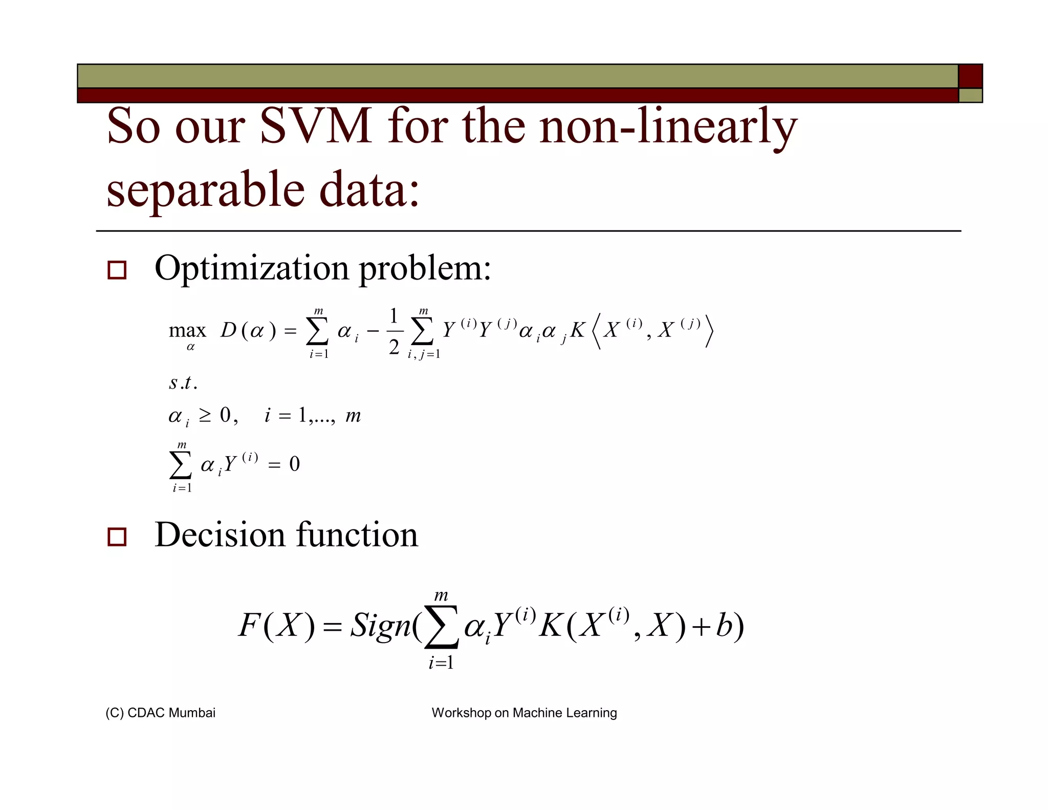
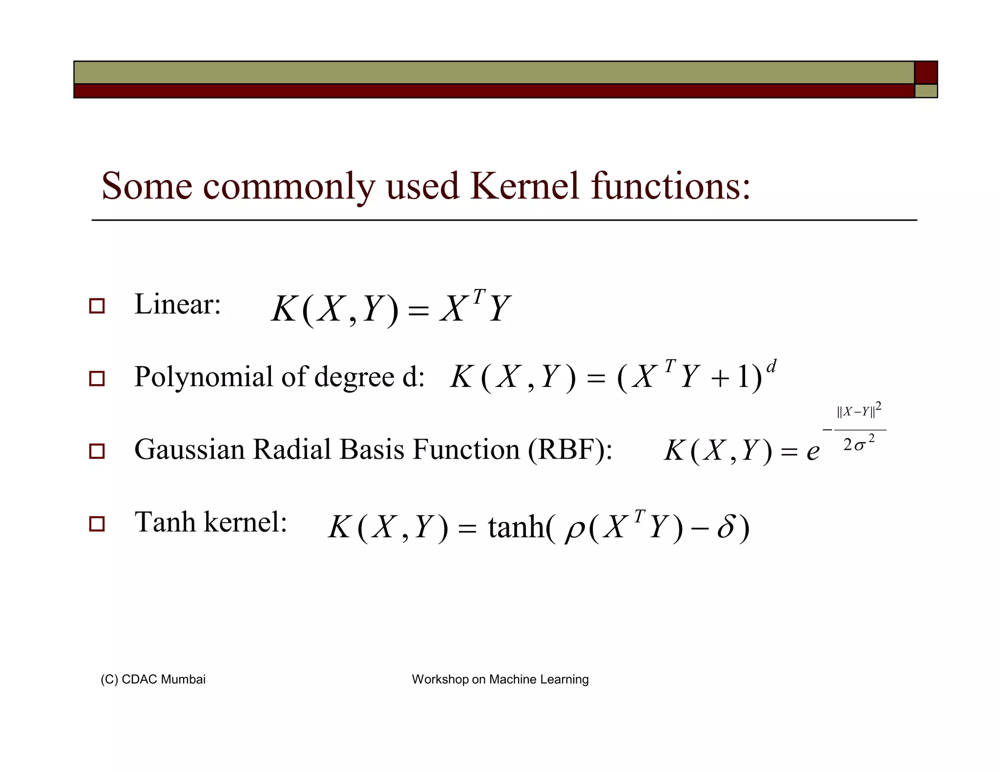
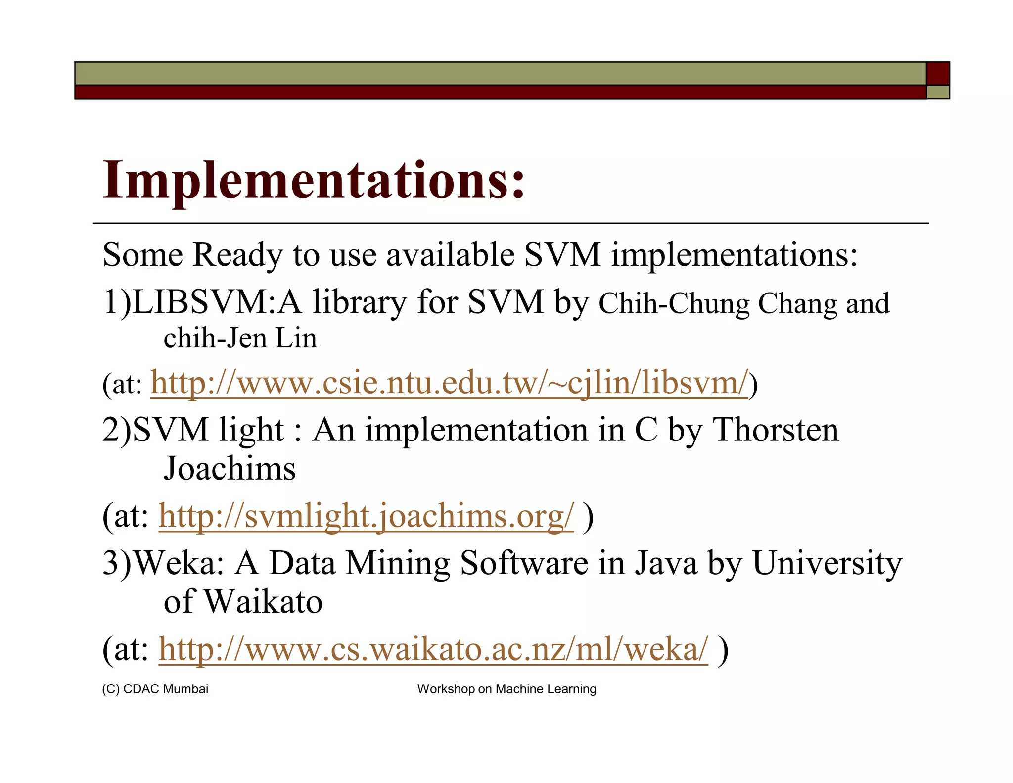
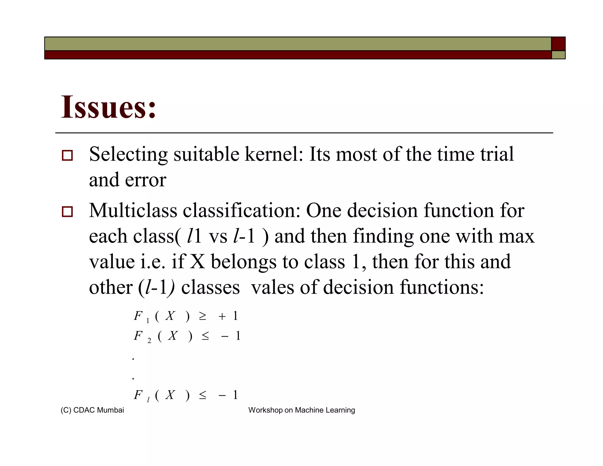
The document provides an overview of support vector machines (SVM), focusing on their theoretical foundation, implementation, and effectiveness for classification and regression tasks. It discusses the Vapnik-Chervonenkis theory, the principles of maximizing the margin between decision boundaries, and various kernel functions used for handling non-linearly separable data. Additionally, it highlights some readily available SVM implementations and common issues encountered when applying these techniques.

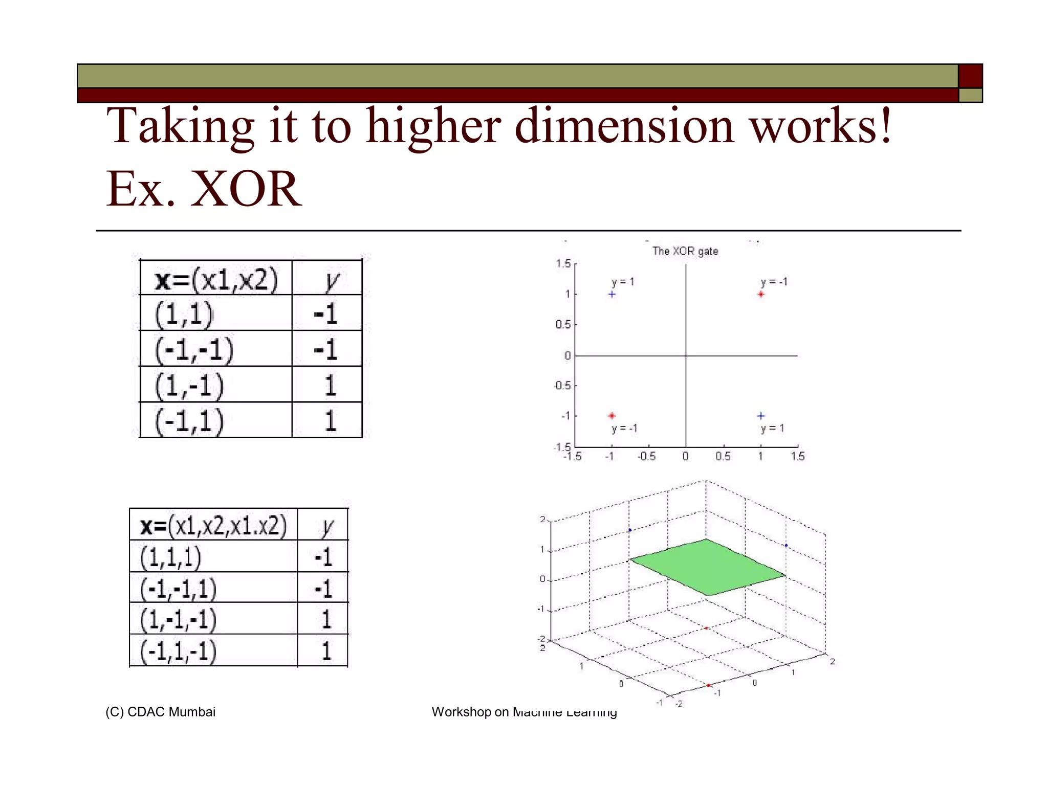
![What it says:
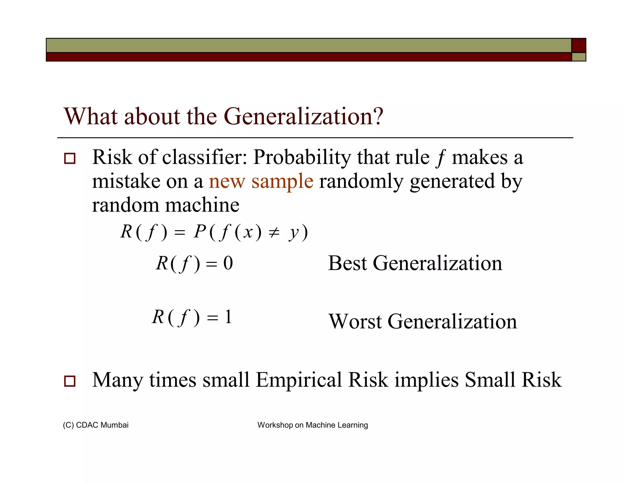
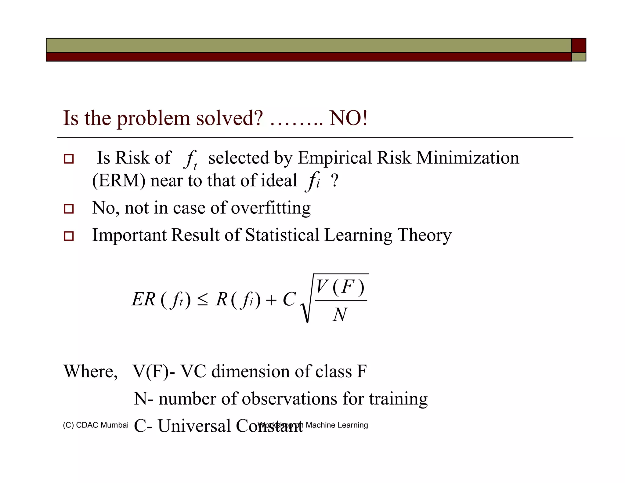
Risk of rule selected by ERM is not far from Risk of
the ideal rule if-
1) N is large enough
2)VC dimension of F should be small enough
(C) CDAC Mumbai Workshop on Machine Learning
2)VC dimension of F should be small enough
[VC dimension? In short larger a class F, the larger its VC dimension (Sorry Vapnik sir!)]](https://image.slidesharecdn.com/svm-130719061500-phpapp02/75/Support-Vector-Machines-for-Classification-8-2048.jpg)
![Constructing Lagrangian
Lagrangian for our problem:
[ ]∑ −+−=
m
iTi
i bXWYWbWL )()(2
1)(||||
2
1
),,( αα
(C) CDAC Mumbai Workshop on Machine Learning
Where a Lagrange multiplier and
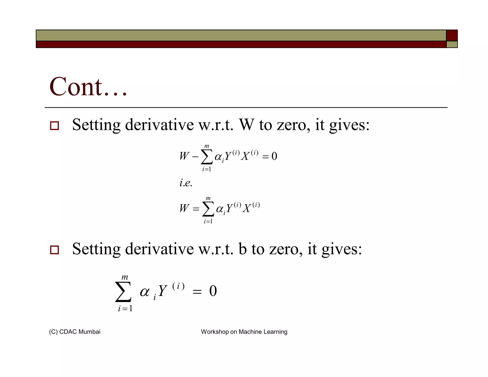
Now minimizing it w.r.t. W and b:
We set derivatives of Lagrangian w.r.t. W and b to zero
[ ]∑=
−+−=
i
i bXWYWbWL
1
1)(||||
2
),,( αα
α 0≥iα](https://image.slidesharecdn.com/svm-130719061500-phpapp02/75/Support-Vector-Machines-for-Classification-23-2048.jpg)
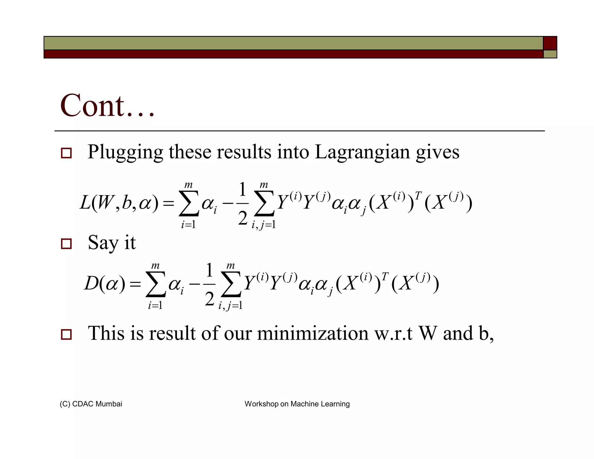
![So The DUAL:
Now Dual becomes::
∑∑ ==
=≥
−=
i
m
ji
ji
ji
ji
m
i
i
mi
ts
XXYYD
1,
)()()()(
1
,...,1,0
..
,
2
1
)(max
α
αααα
α
(C) CDAC Mumbai Workshop on Machine Learning
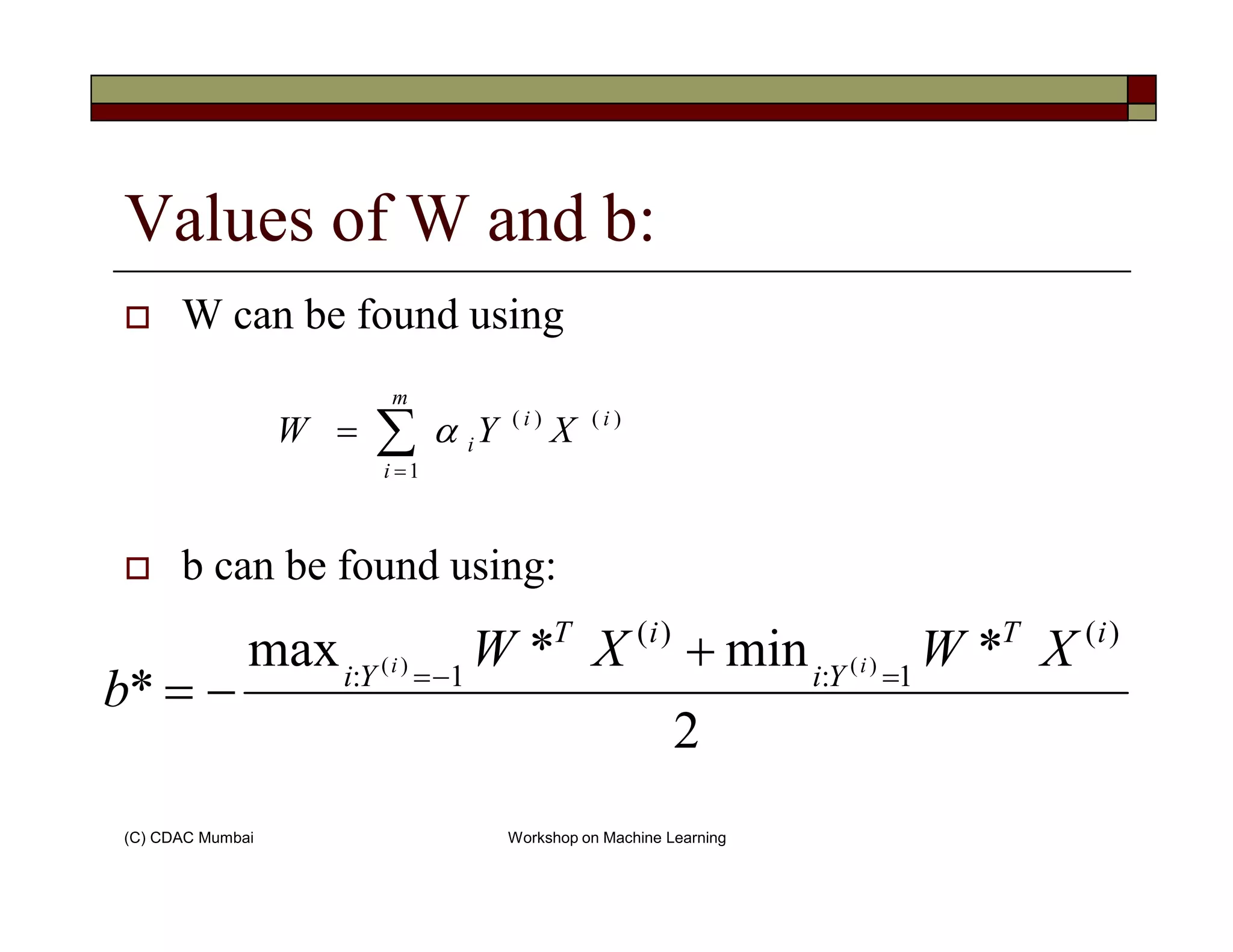
Solving this optimization problem gives us
Also Karush-Kuhn-Tucker (KKT) condition is
satisfied at this solution i.e.
∑=
=
=≥
m
i
i
i
i
Y
mi
1
)(
0
,...,1,0
α
α
iα
[ ] miforbXWY iTi
i ,...,1,01)( )()(
==−+α](https://image.slidesharecdn.com/svm-130719061500-phpapp02/75/Support-Vector-Machines-for-Classification-26-2048.jpg)
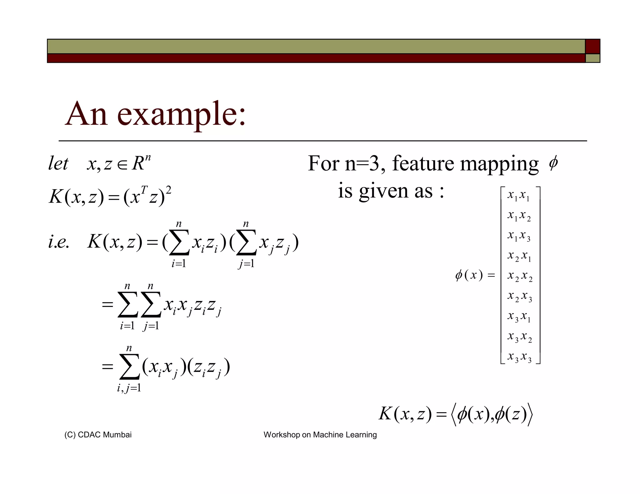
![example cont…
Here,
31
)(),( 2
=
=
=
zx
zxzxK
for
T
4
2
2
1
)(
22
12
21
11
=
=
xx
xx
xx
xx
xφ
(C) CDAC Mumbai Workshop on Machine Learning
[ ]
121)(),(
11
4
3
21
4
3
2
1
2
==
=
=
=
=
zxzxK
zx
zx
T
T
[ ]
121
16
12
12
9
4221)()(
16
12
12
9
)(
=
=
=
zx
z
T
φφ
φ](https://image.slidesharecdn.com/svm-130719061500-phpapp02/75/Support-Vector-Machines-for-Classification-33-2048.jpg)


![[ML]-SVM2.ppt.pdf](https://cdn.slidesharecdn.com/ss_thumbnails/ml-svm2-230916145832-2580c8e3-thumbnail.jpg?width=640&height=640&fit=bounds)


![Vibe Coding vs. Spec-Driven Development [Free Meetup]](https://cdn.slidesharecdn.com/ss_thumbnails/vibecodingvsspecdrivendevelopment-251209105622-43f455e7-thumbnail.jpg?width=640&height=640&fit=bounds)


