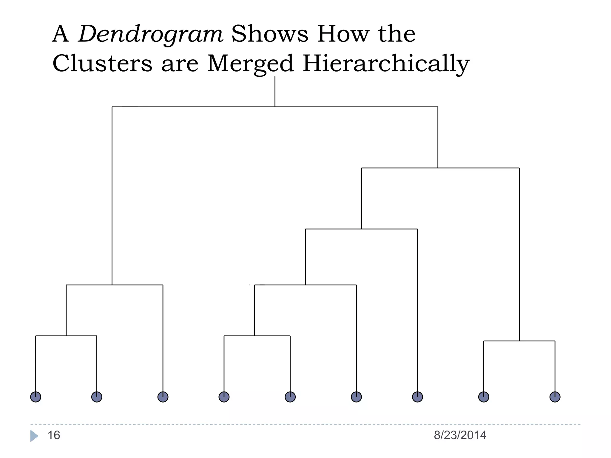
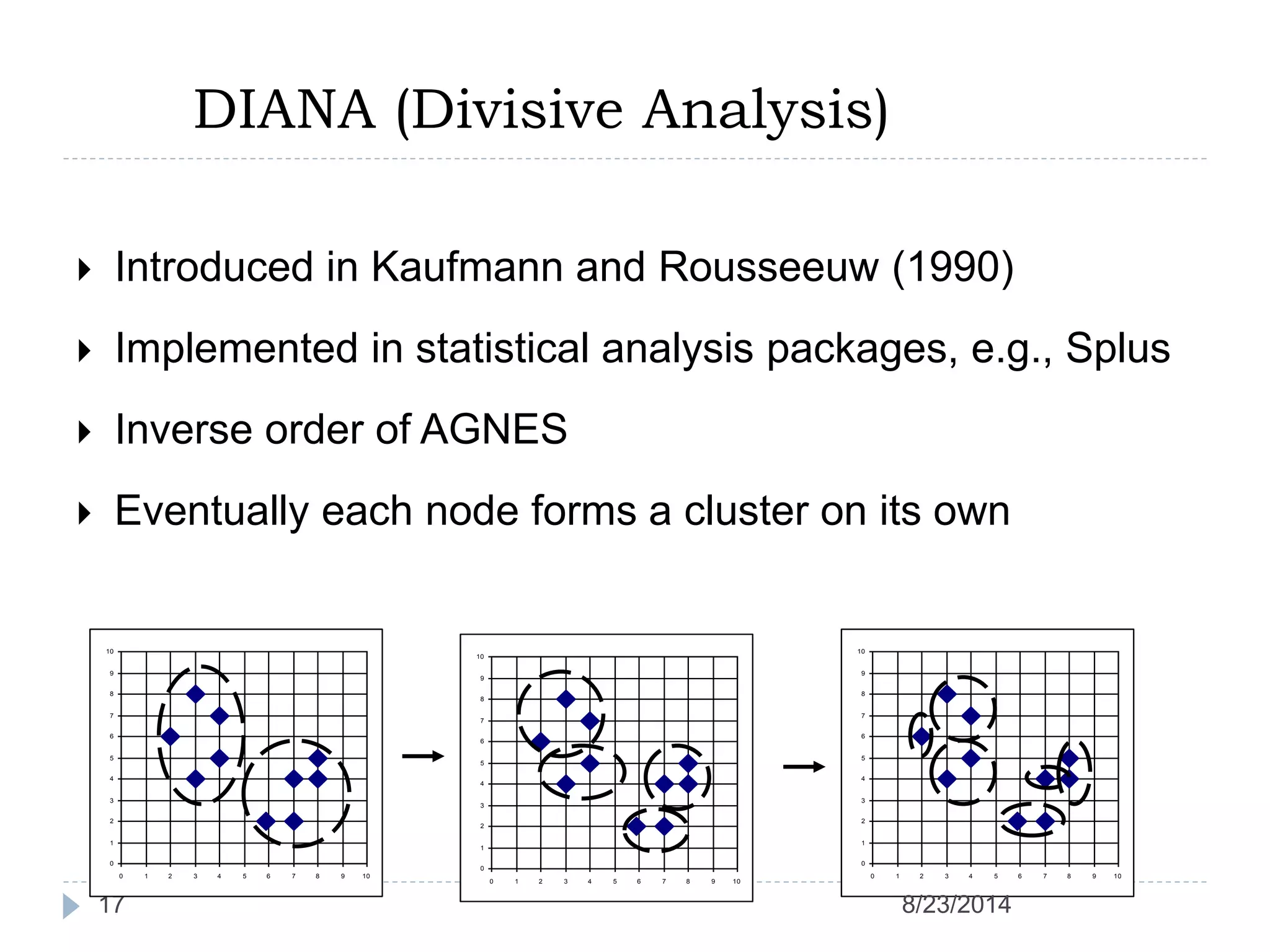
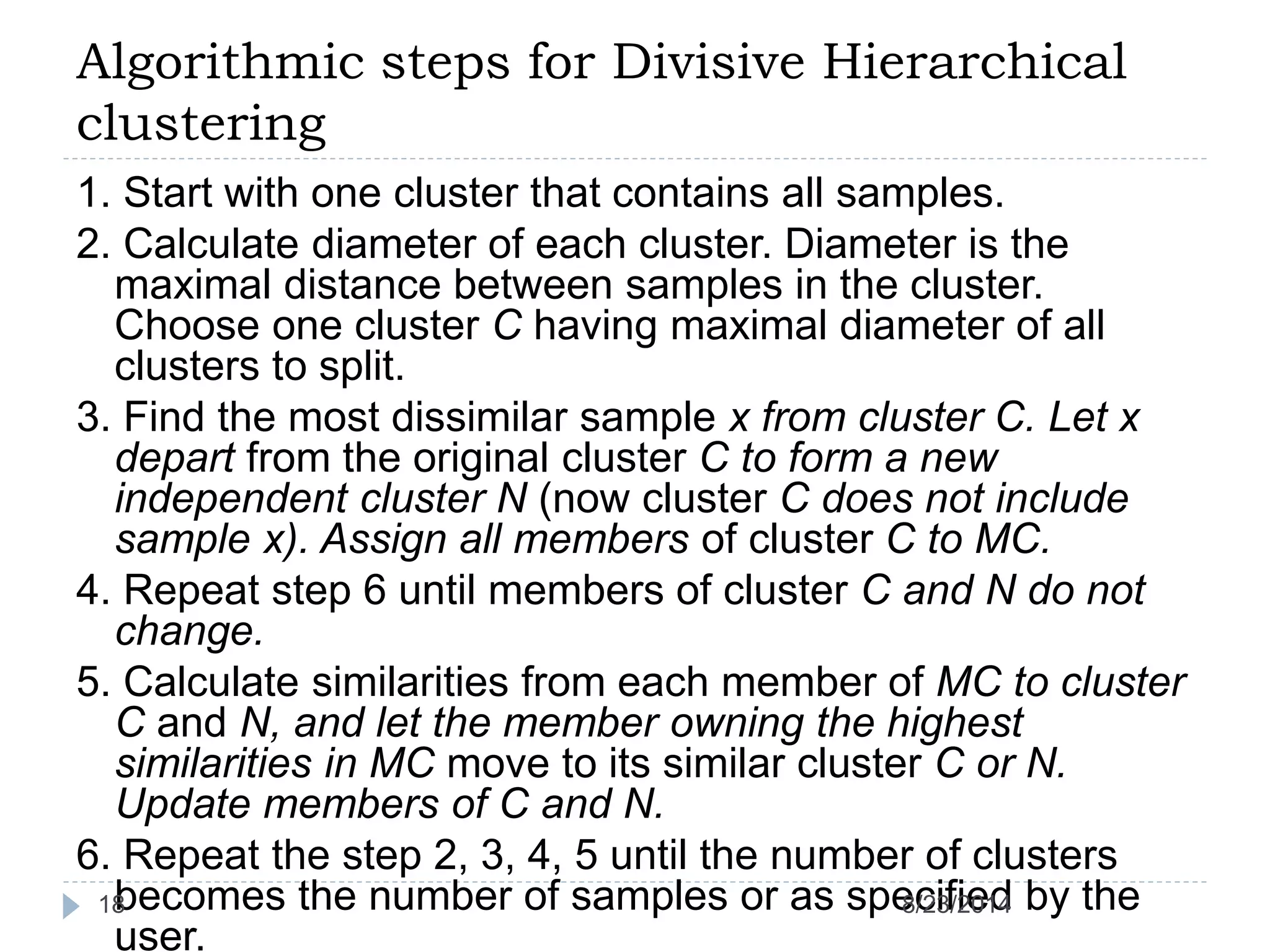
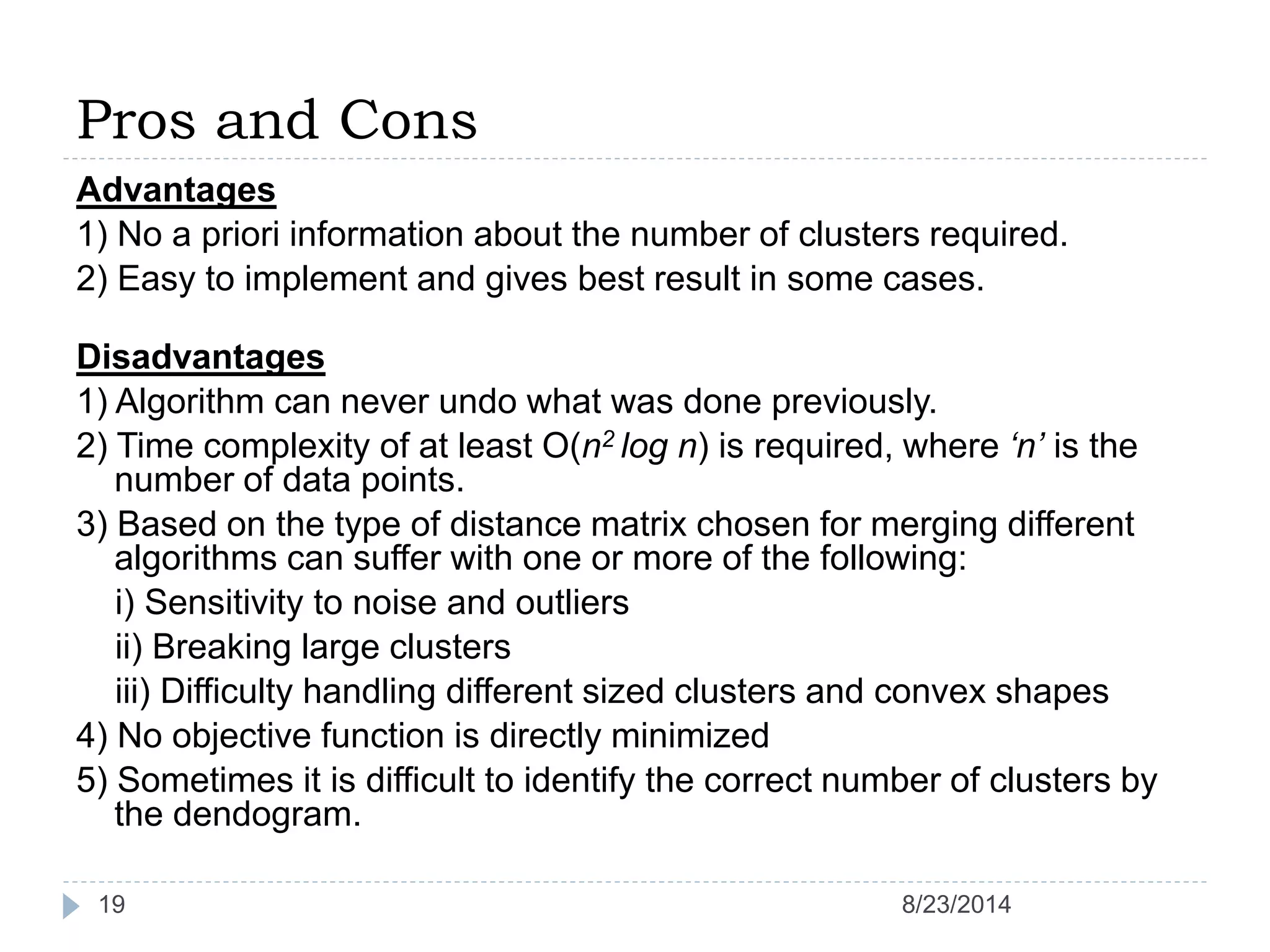
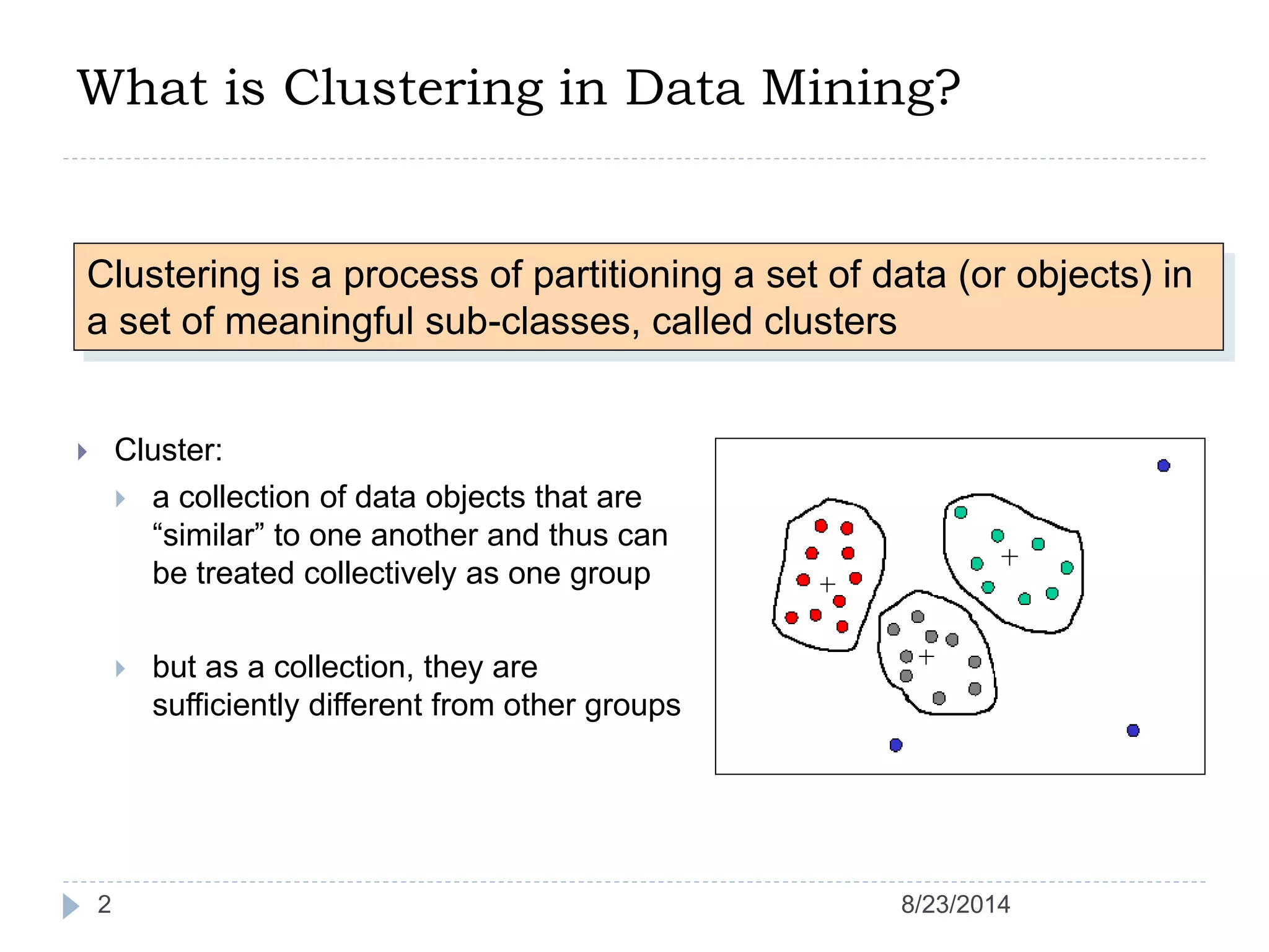
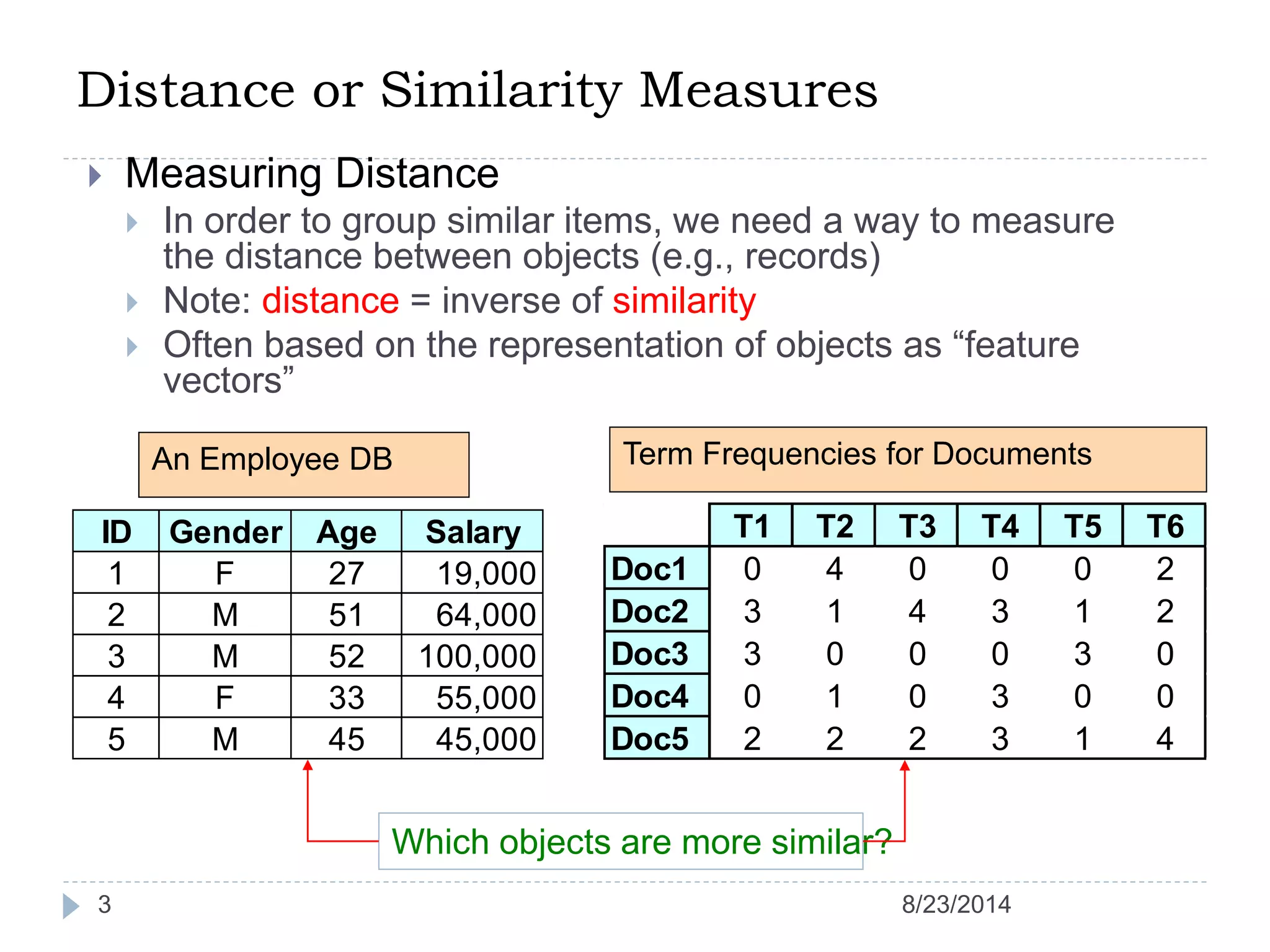
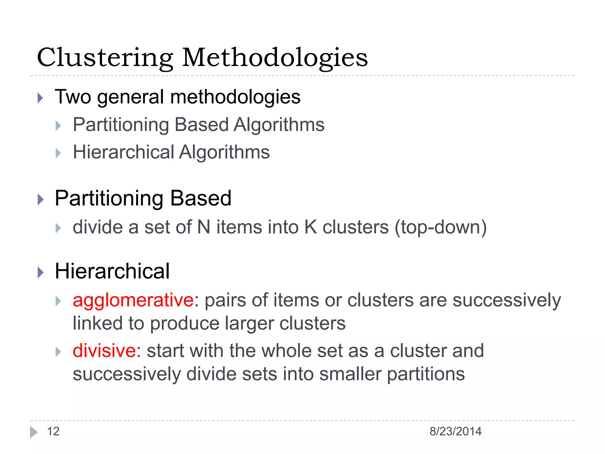
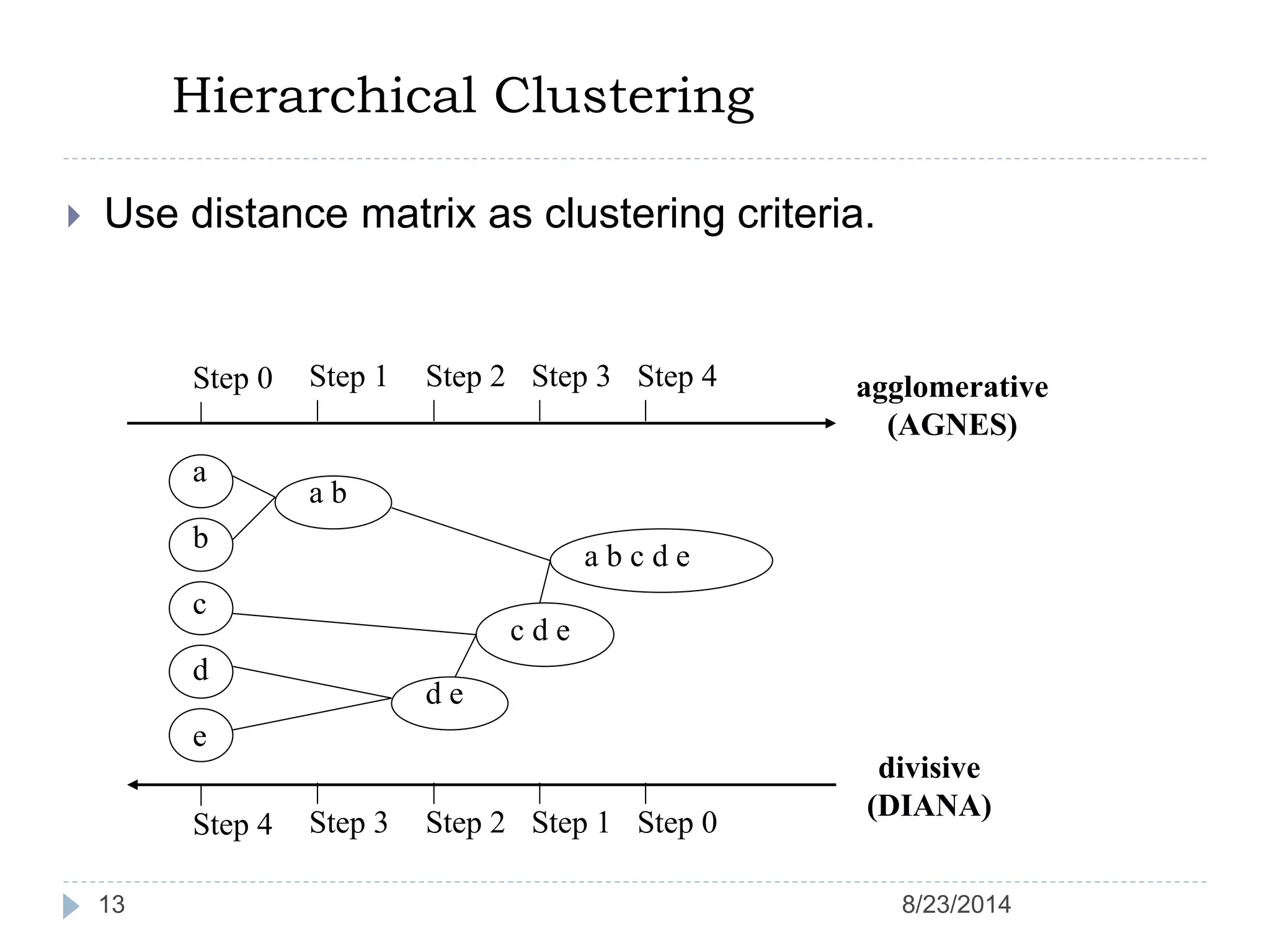
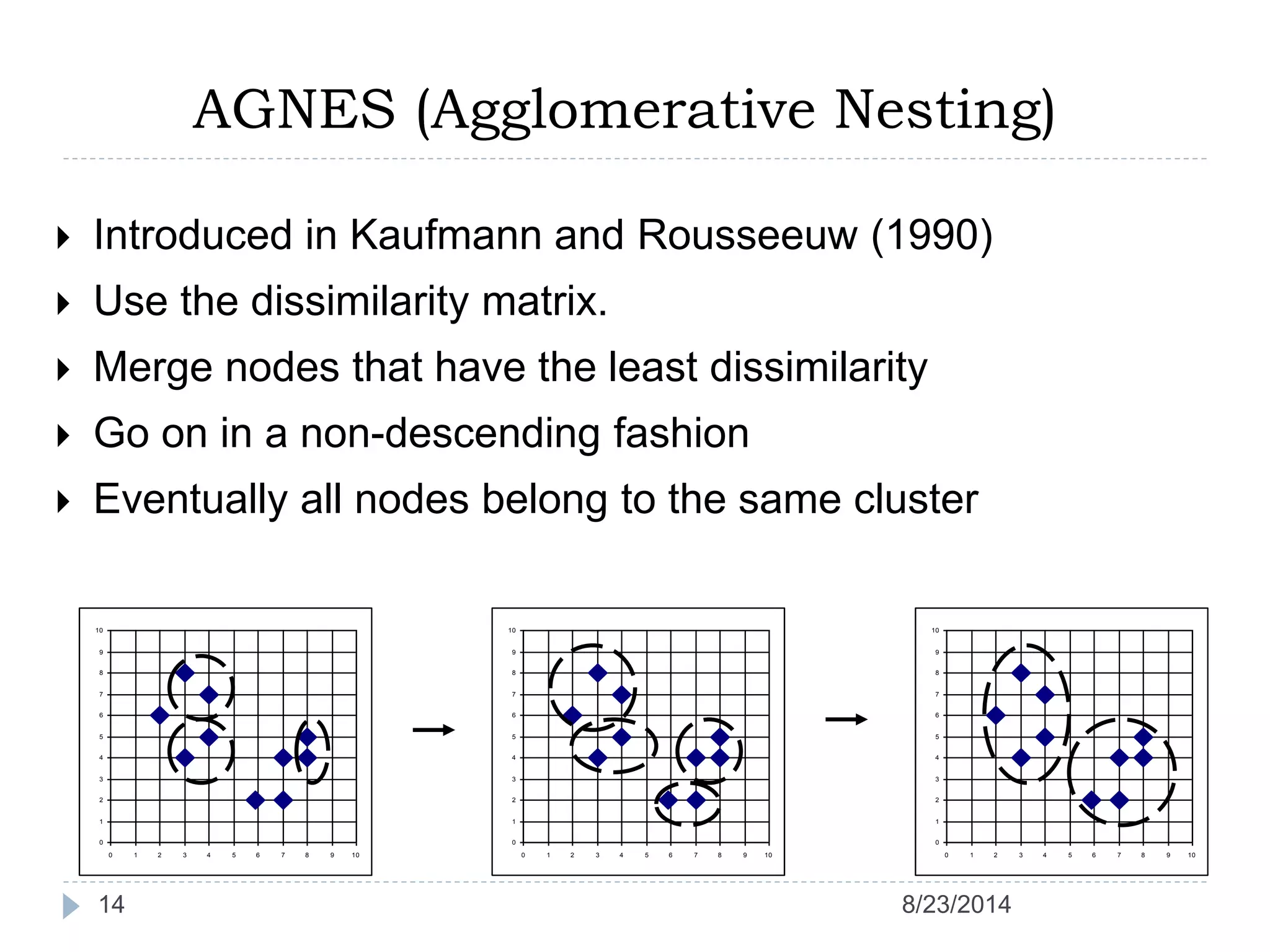
Hierarchical clustering is a method of partitioning a set of data into meaningful sub-classes or clusters. It involves two approaches - agglomerative, which successively links pairs of items or clusters, and divisive, which starts with the whole set as a cluster and divides it into smaller partitions. Agglomerative Nesting (AGNES) is an agglomerative technique that merges clusters with the least dissimilarity at each step, eventually combining all clusters. Divisive Analysis (DIANA) is the inverse, starting with all data in one cluster and splitting it until each data point is its own cluster. Both approaches can be visualized using dendrograms to show the hierarchical merging or splitting of clusters.

1. Hierarchical Clustering
Mehta Ishani
130040701003

2. What is Clustering in Data Mining?
2
 Cluster:
 a collection of data objects that are
“similar” to one another and thus can
be treated collectively as one group
 but as a collection, they are
sufficiently different from other groups
Clustering is a process of partitioning a set of data (or objects) in
a set of meaningful sub-classes, called clusters
8/23/2014

3. Distance or Similarity Measures
3
 Measuring Distance
 In order to group similar items, we need a way to measure
the distance between objects (e.g., records)
 Note: distance = inverse of similarity
 Often based on the representation of objects as “feature
vectors”
ID Gender Age Salary
1 F 27 19,000
2 M 51 64,000
3 M 52 100,000
4 F 33 55,000
5 M 45 45,000
T1 T2 T3 T4 T5 T6
Doc1 0 4 0 0 0 2
Doc2 3 1 4 3 1 2
Doc3 3 0 0 0 3 0
Doc4 0 1 0 3 0 0
Doc5 2 2 2 3 1 4
An Employee DB Term Frequencies for Documents
Which objects are more similar?
8/23/2014

4. Distance or Similarity Measures
4
 Common Distance Measures:
 Manhattan distance:
 Euclidean distance:
 Cosine similarity:
1 2, , , nX x x x 1 2, , , nY y y y
1 1 2 2( , ) n ndist X Y x y x y x y      
   
2 2
1 1( , ) n ndist X Y x y x y    
Can be normalized
to make values fall
between 0 and 1.
( , ) 1 ( , )dist X Y sim X Y 
2 2
( )
( , )
i i
i
i i
i i
x y
sim X Y
x y




 
8/23/2014

5. Distance or Similarity Measures
5
 Weighting Attributes
 in some cases we want some attributes to count more than
others
 associate a weight with each of the attributes in calculating
distance, e.g.,
 Nominal (categorical) Attributes
 can use simple matching: distance=1 if values match, 0
otherwise
 or convert each nominal attribute to a set of binary attribute,
then use the usual distance measure
 if all attributes are nominal, we can normalize by dividing the
number of matches by the total number of attributes
 Normalization:
 want values to fall between 0 an 1:
 other variations possible
   
2 2
1 1 1( , ) n n ndist X Y w x y w x y    
min
'
max min
i i
i
i i
x x
x
x x



8/23/2014

6. Distance or Similarity Measures
6
 Example
 max distance for salary: 100000-19000 = 79000
 max distance for age: 52-27 = 25
 dist(ID2, ID3) = SQRT( 0 + (0.04)2 + (0.44)2 ) = 0.44
 dist(ID2, ID4) = SQRT( 1 + (0.72)2 + (0.12)2 ) = 1.24
ID Gender Age Salary
1 F 27 19,000
2 M 51 64,000
3 M 52 100,000
4 F 33 55,000
5 M 45 45,000
min
'
max min
i i
i
i i
x x
x
x x



ID Gender Age Salary
1 1 0.00 0.00
2 0 0.96 0.56
3 0 1.00 1.00
4 1 0.24 0.44
5 0 0.72 0.32
8/23/2014

7. Domain Specific Distance Functions
7
 For some data sets, we may need to use specialized functions
 we may want a single or a selected group of attributes to be used
in the computation of distance - same problem as “feature
selection”
 may want to use special properties of one or more attribute in the
data
 natural distance functions may exist in the data
Example: Zip Codes
distzip(A, B) = 0, if zip codes are identical
distzip(A, B) = 0.1, if first 3 digits are
identical
distzip(A, B) = 0.5, if first digits are identical
distzip(A, B) = 1, if first digits are different
Example: Customer Solicitation
distsolicit(A, B) = 0, if both A and B responded
distsolicit(A, B) = 0.1, both A and B were chosen but did not respond
distsolicit(A, B) = 0.5, both A and B were chosen, but only one
responded
distsolicit(A, B) = 1, one was chosen, but the other was not
8/23/2014

8. Distance (Similarity) Matrix
8
 Similarity (Distance) Matrix
 based on the distance or similarity measure we can construct a
symmetric matrix of distance (or similarity values)
 (i, j) entry in the matrix is the distance (similarity) between items
i and j
similarity (or distance) of toij i jd D D
Note that dij = dji (i.e., the matrix is
symmetric. So, we only need the
lower triangle part of the matrix.
The diagonal is all 1’s (similarity) or
all 0’s (distance)
1 2
1 12 1
2 21 2
1 2
n
n
n
n n n
I I I
I d d
I d d
I d d




8/23/2014

9. Example: Term Similarities in Documents
9
T1 T2 T3 T4 T5 T6 T7 T8
Doc1 0 4 0 0 0 2 1 3
Doc2 3 1 4 3 1 2 0 1
Doc3 3 0 0 0 3 0 3 0
Doc4 0 1 0 3 0 0 2 0
Doc5 2 2 2 3 1 4 0 2
sim T T w wi j jkik
k
N
( , ) ( ) 


1
T1 T2 T3 T4 T5 T6 T7
T2 7
T3 16 8
T4 15 12 18
T5 14 3 6 6
T6 14 18 16 18 6
T7 9 6 0 6 9 2
T8 7 17 8 9 3 16 3
Term-Term
Similarity Matrix
8/23/2014

10. Similarity (Distance) Thresholds
10
 A similarity (distance) threshold may be used to mark pairs that are
“sufficiently” similarT1 T2 T3 T4 T5 T6 T7
T2 7
T3 16 8
T4 15 12 18
T5 14 3 6 6
T6 14 18 16 18 6
T7 9 6 0 6 9 2
T8 7 17 8 9 3 16 3
T1 T2 T3 T4 T5 T6 T7
T2 0
T3 1 0
T4 1 1 1
T5 1 0 0 0
T6 1 1 1 1 0
T7 0 0 0 0 0 0
T8 0 1 0 0 0 1 0
Using a
threshold value
of 10 in the
previous
example
8/23/2014

11. Graph Representation
11
 The similarity matrix can be visualized as an undirected
graph
 each item is represented by a node, and edges represent the
fact that two items are similar (a one in the similarity threshold
matrix)
T1 T2 T3 T4 T5 T6 T7
T2 0
T3 1 0
T4 1 1 1
T5 1 0 0 0
T6 1 1 1 1 0
T7 0 0 0 0 0 0
T8 0 1 0 0 0 1 0
T1 T3
T4
T6
T8
T5
T2
T7
If no threshold is used, then
matrix can be represented as
a weighted graph
8/23/2014

12. Clustering Methodologies
12
 Two general methodologies
 Partitioning Based Algorithms
 Hierarchical Algorithms
 Partitioning Based
 divide a set of N items into K clusters (top-down)
 Hierarchical
 agglomerative: pairs of items or clusters are successively
linked to produce larger clusters
 divisive: start with the whole set as a cluster and
successively divide sets into smaller partitions
8/23/2014

13. Hierarchical Clustering
13
 Use distance matrix as clustering criteria.
Step 0 Step 1 Step 2 Step 3 Step 4
b
d
c
e
a
a b
d e
c d e
a b c d e
Step 4 Step 3 Step 2 Step 1 Step 0
agglomerative
(AGNES)
divisive
(DIANA)
8/23/2014

14. AGNES (Agglomerative Nesting)
14
 Introduced in Kaufmann and Rousseeuw (1990)
 Use the dissimilarity matrix.
 Merge nodes that have the least dissimilarity
 Go on in a non-descending fashion
 Eventually all nodes belong to the same cluster
0
1
2
3
4
5
6
7
8
9
10
0 1 2 3 4 5 6 7 8 9 10
0
1
2
3
4
5
6
7
8
9
10
0 1 2 3 4 5 6 7 8 9 10
0
1
2
3
4
5
6
7
8
9
10
0 1 2 3 4 5 6 7 8 9 10
8/23/2014

15. Algorithmic steps for Agglomerative
Hierarchical clustering
Let X = {x1, x2, x3, ..., xn} be the set of data points.
(1)Begin with the disjoint clustering having level L(0) = 0 and sequence number m =
0.
(2)Find the least distance pair of clusters in the current clustering, say pair (r), (s),
according
to d[(r),(s)] = min d[(i),(j)] where the minimum is over all pairs of clusters in
the current clustering.
(3)Increment the sequence number: m = m +1.Merge clusters (r) and (s) into a
single cluster to form the next clustering m. Set the level of this clustering to
L(m) = d[(r),(s)].
(4)Update the distance matrix, D, by deleting the rows and columns corresponding
to clusters (r) and (s) and adding a row and column corresponding to the
newly formed cluster. The distance between the new cluster, denoted (r,s) and
old cluster(k) is defined in this way: d[(k), (r,s)] = min (d[(k),(r)], d[(k),(s)]).
(5)If all the data points are in one cluster then stop, else repeat from step 2).8/23/201415

16. 16
A Dendrogram Shows How the
Clusters are Merged Hierarchically
8/23/2014

17. DIANA (Divisive Analysis)
17
 Introduced in Kaufmann and Rousseeuw (1990)
 Implemented in statistical analysis packages, e.g., Splus
 Inverse order of AGNES
 Eventually each node forms a cluster on its own
0
1
2
3
4
5
6
7
8
9
10
0 1 2 3 4 5 6 7 8 9 10
0
1
2
3
4
5
6
7
8
9
10
0 1 2 3 4 5 6 7 8 9 10
0
1
2
3
4
5
6
7
8
9
10
0 1 2 3 4 5 6 7 8 9 10
8/23/2014

18. Algorithmic steps for Divisive Hierarchical
clustering
1. Start with one cluster that contains all samples.
2. Calculate diameter of each cluster. Diameter is the
maximal distance between samples in the cluster.
Choose one cluster C having maximal diameter of all
clusters to split.
3. Find the most dissimilar sample x from cluster C. Let x
depart from the original cluster C to form a new
independent cluster N (now cluster C does not include
sample x). Assign all members of cluster C to MC.
4. Repeat step 6 until members of cluster C and N do not
change.
5. Calculate similarities from each member of MC to cluster
C and N, and let the member owning the highest
similarities in MC move to its similar cluster C or N.
Update members of C and N.
6. Repeat the step 2, 3, 4, 5 until the number of clusters
becomes the number of samples or as specified by the
user.
8/23/201418

19. Pros and Cons
Advantages
1) No a priori information about the number of clusters required.
2) Easy to implement and gives best result in some cases.
Disadvantages
1) Algorithm can never undo what was done previously.
2) Time complexity of at least O(n2 log n) is required, where ‘n’ is the
number of data points.
3) Based on the type of distance matrix chosen for merging different
algorithms can suffer with one or more of the following:
i) Sensitivity to noise and outliers
ii) Breaking large clusters
iii) Difficulty handling different sized clusters and convex shapes
4) No objective function is directly minimized
5) Sometimes it is difficult to identify the correct number of clusters by
the dendogram.
8/23/201419

20. 8/23/201420