Downloaded 10,681 times


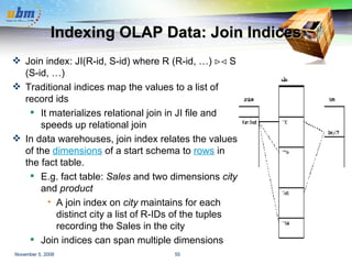
![Cube Definition Syntax (BNF) in DMQL Cube Definition (Fact Table) define cube <cube_name> [<dimension_list>]: <measure_list> Dimension Definition (Dimension Table) define dimension <dimension_name> as (<attribute_or_subdimension_list>) Special Case (Shared Dimension Tables) First time as “cube definition” define dimension <dimension_name> as <dimension_name_first_time> in cube <cube_name_first_time>](https://image.slidesharecdn.com/yoyopresentasi-1225941108853502-8/85/Data-Warehousing-and-Data-Mining-24-320.jpg)
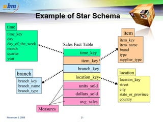
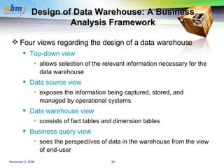
![Defining Star Schema in DMQL define cube sales_star [time, item, branch, location]: dollars_sold = sum(sales_in_dollars), avg_sales = avg(sales_in_dollars), units_sold = count(*) define dimension time as (time_key, day, day_of_week, month, quarter, year) define dimension item as (item_key, item_name, brand, type, supplier_type) define dimension branch as (branch_key, branch_name, branch_type) define dimension location as (location_key, street, city, province_or_state, country)](https://image.slidesharecdn.com/yoyopresentasi-1225941108853502-8/85/Data-Warehousing-and-Data-Mining-25-320.jpg)
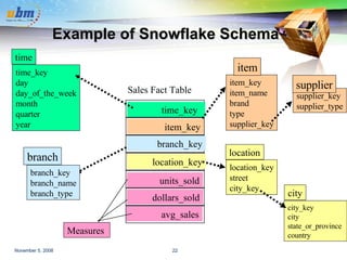
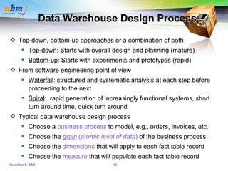
![Defining Snowflake Schema in DMQL define cube sales_snowflake [time, item, branch, location]: dollars_sold = sum(sales_in_dollars), avg_sales = avg(sales_in_dollars), units_sold = count(*) define dimension time as (time_key, day, day_of_week, month, quarter, year) define dimension item as (item_key, item_name, brand, type, supplier(supplier_key, supplier_type)) define dimension branch as (branch_key, branch_name, branch_type) define dimension location as (location_key, street, city(city_key, province_or_state, country))](https://image.slidesharecdn.com/yoyopresentasi-1225941108853502-8/85/Data-Warehousing-and-Data-Mining-26-320.jpg)
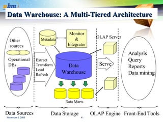
![Defining Fact Constellation in DMQL define cube sales [time, item, branch, location]: dollars_sold = sum(sales_in_dollars), avg_sales = avg(sales_in_dollars), units_sold = count(*) define dimension time as (time_key, day, day_of_week, month, quarter, year) define dimension item as (item_key, item_name, brand, type, supplier_type) define dimension branch as (branch_key, branch_name, branch_type) define dimension location as (location_key, street, city, province_or_state, country) define cube shipping [time, item, shipper, from_location, to_location]: dollar_cost = sum(cost_in_dollars), unit_shipped = count(*) define dimension time as time in cube sales define dimension item as item in cube sales define dimension shipper as (shipper_key, shipper_name, location as location in cube sales, shipper_type) define dimension from_location as location in cube sales define dimension to_location as location in cube sales](https://image.slidesharecdn.com/yoyopresentasi-1225941108853502-8/85/Data-Warehousing-and-Data-Mining-27-320.jpg)
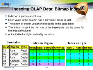
![Cube Operation Cube definition and computation in DMQL define cube sales[item, city, year]: sum(sales_in_dollars) compute cube sales Transform it into a SQL-like language (with a new operator cube by , introduced by Gray et al.’96) SELECT item, city, year, SUM (amount) FROM SALES CUBE BY item, city, year Need compute the following Group-Bys ( date, product, customer), (date,product),(date, customer), (product, customer), (date), (product), (customer) () (item) (city) () (year) (city, item) (city, year) (item, year) (city, item, year)](https://image.slidesharecdn.com/yoyopresentasi-1225941108853502-8/85/Data-Warehousing-and-Data-Mining-52-320.jpg)


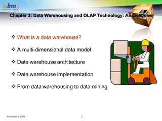
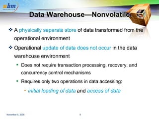
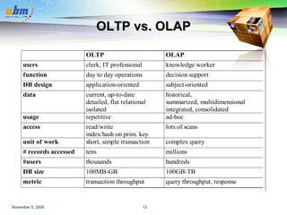
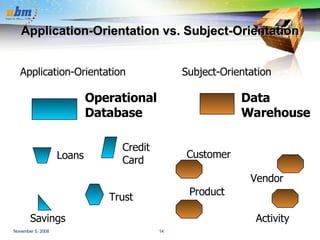
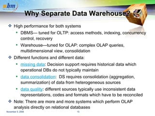
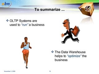
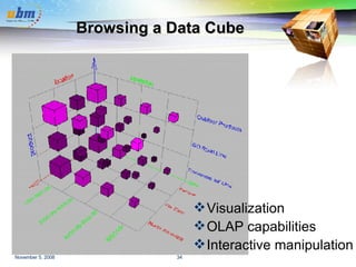
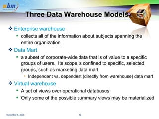
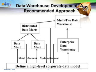
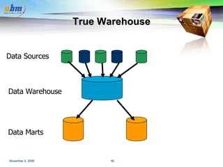
This document discusses data warehousing and OLAP (online analytical processing) technology. It defines a data warehouse as a subject-oriented, integrated, time-variant, and nonvolatile collection of data to support management decision making. It describes how data warehouses use a multi-dimensional data model with facts and dimensions to organize historical data from multiple sources for analysis. Common data warehouse architectures like star schemas and snowflake schemas are also summarized.


