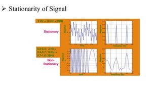
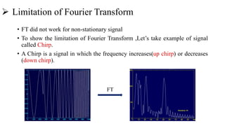
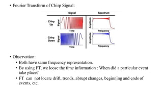
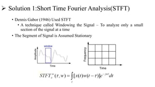
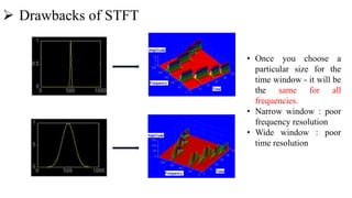
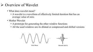
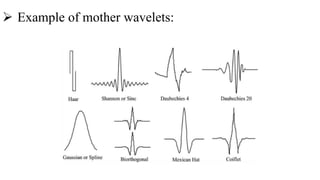
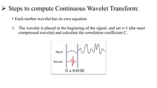
INTRODUCTION TO WAVELET TRANSFORM
OUTLINE
• Overview
• Limitation of Fourier transform
• Overview of Wavelet
• Principle of Wavelet Transform
• Continuous Wavelet Transform (CWT)
• Discrete Wavelet Transform (DWT)
• Applications
• Advantages
 Stationarity of Signal
 Limitation of Fourier Transform
• FT did not work for non-stationary signal
• To show the limitation of Fourier Transform ,Let’s take example of signal
called Chirp.
• A Chirp is a signal in which the frequency increases(up chirp) or decreases
(down chirp).
FT
• Fourier Transform of Chirp Signal:
• Observation:
• Both have same frequency representation.
• By using FT, we loose the time information : When did a particular event
take place?
• FT can not locate drift, trends, abrupt changes, beginning and ends of
events, etc.
 Solution 1:Short Time Fourier Analysis(STFT)
• Dennis Gabor (1946) Used STFT
• A technique called Windowing the Signal – To analyze only a small
section of the signal at a time
• The Segment of Signal is Assumed Stationary
 Drawbacks of STFT
• Once you choose a
particular size for the
time window - it will be
the same for all
frequencies.
• Narrow window : poor
frequency resolution
• Wide window : poor
time resolution
 Overview of Wavelet
• What does wavelet mean?
• A wavelet is a waveform of effectively limited duration that has an
average value of zero.
• Mother Wavelet
• A prototype for generating the other window functions
• All the used windows are its dilated or compressed and shifted versions
 Example of mother wavelets:
 Principle of Wavelet Transform:
• Split Up the Signal into a Bunch of Signals
• Representing the Same Signal, but all Corresponding to Different
Frequency Bands
• Only Providing What Frequency Bands Exists at What Time Intervals
• DEFINITION OF CONTINUOUS WAVELET TRANSFORM:
𝐶𝑊𝑇𝑥
𝜓
(𝜏 , 𝑠 ) = 𝛹𝑥
𝜓
(𝜏 , 𝑠 ) =
1
𝑆
𝑥 𝑡 ● 𝛹
𝑡 − 𝜏
𝑠
dt
where,
S=scale
• S > 1:dialate the signal
• S < 1:compress the signal
τ= translation
Ψ
t − τ
s
= mother wavelet
 Steps to compute Continuous Wavelet Transform:
• Each mother wavelet has its own equation
1. The wavelet is placed at the beginning of the signal, and set s=1 (the most
compressed wavelet) and calculate the correlation coefficient C.
2. Shift the wavelet to the right and repeat step 1 until the whole signal is
covered.
3. Scale s is increased by a sufficiently small value, the above procedure is
repeated for all s.
4. Repeat steps 1 to 3 for all scales.
Fig. the signal and the wavelet function are
shown for four different values of τ . The scale
value is 1, corresponding to the lowest scale,
or highest frequency.
Fig. The wavelet function with scale value of
20.The increased value of scale corresponds to
the lowest frequency.
Fig. Signal is composed of four different
frequency at 30 Hz, 20 Hz, 10 Hz and 5
Hz.
Fig. Continuous wavelet transform of the signal.
 Time and Frequency Resolution:
• lower scales (higher frequencies) have better scale resolution which correspond to
poorer frequency resolution. Similarly, higher scales have poorer scale
frequency which correspond to better frequency resolution of lower frequencies.
 Discrete Wavelet Transform
• Filters of different cutoff frequencies are used to analyze the signal
𝑥 𝑛 ∗ ℎ 𝑛 = 𝑘=−∞
∞
𝑥 𝑘 ● ℎ 𝑛 − 𝑘
• The signal is passed through a series of high pass filters to analyze the high
frequencies, and it is passed through a series of low pass filters to analyze
the low frequencies.
𝑦ℎ𝑖𝑔ℎ 𝑘 = 𝑛 𝑥 𝑛 ● 𝑔 2𝑘 − 𝑛
𝑦𝑙𝑜𝑤 𝑘 = 𝑛 𝑥 𝑛 ● ℎ 2𝑘 − 𝑛
where 𝑦ℎ𝑖𝑔ℎ 𝑘 and 𝑦𝑙𝑜𝑤 𝑘 are the outputs of the high pass and low pass filters,
respectively, after subsampling by 2.
• x[n] is the original signal to be decomposed
• h[n] and g[n] are low pass and high pass filters.
• The bandwidth of the signal at every level is
marked on the figure as "f".
• At every level, the filtering and subsampling
will result in half the number of samples (and
hence half the time resolution) and half the
frequency band spanned (and hence double the
frequency resolution).
 Applications:
• Image and signal Compression
• Image and signal Denoising
• Calculate the DWT of the image
• Threshold the wavelet coefficients.
• Compute the IDWT to get the denoised image.
• Time frequency Analysis
 Advantages:
• Provide a way for analyzing waveform in both time and frequency
duration.
• Provide a way to reconstruct finite, non-stationary and non-periodic
signal.
• Allow signal to be stored more efficiently compare to Fourier
transform.
Wavelet transform

Wavelet transform

  • 1.
  • 2.
    OUTLINE • Overview • Limitationof Fourier transform • Overview of Wavelet • Principle of Wavelet Transform • Continuous Wavelet Transform (CWT) • Discrete Wavelet Transform (DWT) • Applications • Advantages
  • 3.
  • 4.
     Limitation ofFourier Transform • FT did not work for non-stationary signal • To show the limitation of Fourier Transform ,Let’s take example of signal called Chirp. • A Chirp is a signal in which the frequency increases(up chirp) or decreases (down chirp). FT
  • 5.
    • Fourier Transformof Chirp Signal: • Observation: • Both have same frequency representation. • By using FT, we loose the time information : When did a particular event take place? • FT can not locate drift, trends, abrupt changes, beginning and ends of events, etc.
  • 6.
     Solution 1:ShortTime Fourier Analysis(STFT) • Dennis Gabor (1946) Used STFT • A technique called Windowing the Signal – To analyze only a small section of the signal at a time • The Segment of Signal is Assumed Stationary
  • 7.
     Drawbacks ofSTFT • Once you choose a particular size for the time window - it will be the same for all frequencies. • Narrow window : poor frequency resolution • Wide window : poor time resolution
  • 8.
     Overview ofWavelet • What does wavelet mean? • A wavelet is a waveform of effectively limited duration that has an average value of zero. • Mother Wavelet • A prototype for generating the other window functions • All the used windows are its dilated or compressed and shifted versions
  • 9.
     Example ofmother wavelets:
  • 10.
     Principle ofWavelet Transform: • Split Up the Signal into a Bunch of Signals • Representing the Same Signal, but all Corresponding to Different Frequency Bands • Only Providing What Frequency Bands Exists at What Time Intervals • DEFINITION OF CONTINUOUS WAVELET TRANSFORM: 𝐶𝑊𝑇𝑥 𝜓 (𝜏 , 𝑠 ) = 𝛹𝑥 𝜓 (𝜏 , 𝑠 ) = 1 𝑆 𝑥 𝑡 ● 𝛹 𝑡 − 𝜏 𝑠 dt where, S=scale • S > 1:dialate the signal • S < 1:compress the signal τ= translation Ψ t − τ s = mother wavelet
  • 11.
     Steps tocompute Continuous Wavelet Transform: • Each mother wavelet has its own equation 1. The wavelet is placed at the beginning of the signal, and set s=1 (the most compressed wavelet) and calculate the correlation coefficient C.
  • 12.
    2. Shift thewavelet to the right and repeat step 1 until the whole signal is covered. 3. Scale s is increased by a sufficiently small value, the above procedure is repeated for all s. 4. Repeat steps 1 to 3 for all scales.
  • 13.
    Fig. the signaland the wavelet function are shown for four different values of τ . The scale value is 1, corresponding to the lowest scale, or highest frequency. Fig. The wavelet function with scale value of 20.The increased value of scale corresponds to the lowest frequency.
  • 14.
    Fig. Signal iscomposed of four different frequency at 30 Hz, 20 Hz, 10 Hz and 5 Hz. Fig. Continuous wavelet transform of the signal.
  • 15.
     Time andFrequency Resolution: • lower scales (higher frequencies) have better scale resolution which correspond to poorer frequency resolution. Similarly, higher scales have poorer scale frequency which correspond to better frequency resolution of lower frequencies.
  • 16.
     Discrete WaveletTransform • Filters of different cutoff frequencies are used to analyze the signal 𝑥 𝑛 ∗ ℎ 𝑛 = 𝑘=−∞ ∞ 𝑥 𝑘 ● ℎ 𝑛 − 𝑘 • The signal is passed through a series of high pass filters to analyze the high frequencies, and it is passed through a series of low pass filters to analyze the low frequencies. 𝑦ℎ𝑖𝑔ℎ 𝑘 = 𝑛 𝑥 𝑛 ● 𝑔 2𝑘 − 𝑛 𝑦𝑙𝑜𝑤 𝑘 = 𝑛 𝑥 𝑛 ● ℎ 2𝑘 − 𝑛 where 𝑦ℎ𝑖𝑔ℎ 𝑘 and 𝑦𝑙𝑜𝑤 𝑘 are the outputs of the high pass and low pass filters, respectively, after subsampling by 2.
  • 17.
    • x[n] isthe original signal to be decomposed • h[n] and g[n] are low pass and high pass filters. • The bandwidth of the signal at every level is marked on the figure as "f". • At every level, the filtering and subsampling will result in half the number of samples (and hence half the time resolution) and half the frequency band spanned (and hence double the frequency resolution).
  • 18.
     Applications: • Imageand signal Compression • Image and signal Denoising • Calculate the DWT of the image • Threshold the wavelet coefficients. • Compute the IDWT to get the denoised image. • Time frequency Analysis
  • 19.
     Advantages: • Providea way for analyzing waveform in both time and frequency duration. • Provide a way to reconstruct finite, non-stationary and non-periodic signal. • Allow signal to be stored more efficiently compare to Fourier transform.