


![Properties of S matrix
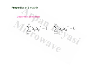
Under perfect matched condition,
diagonal elements of [S] are equal to ‘0’
0
ii
S ](https://image.slidesharecdn.com/scatteringmatrix-210220134538/85/Scattering-matrix-22-320.jpg)
![Properties of S matrix
[S] is symmetric for all reciprocal networks
T
S S
ij ji
S S
ii ij ii ji
ji jj ij jj
S S S S
S S S S
](https://image.slidesharecdn.com/scatteringmatrix-210220134538/85/Scattering-matrix-23-320.jpg)
![Properties of S matrix
For lossless network, [S] matrix is unitary
*
S S I
*
1 0
0 1
ii ij ii ij
ji jj ji jj
S S S S
S S S S
](https://image.slidesharecdn.com/scatteringmatrix-210220134538/85/Scattering-matrix-24-320.jpg)
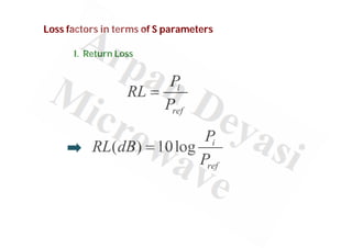
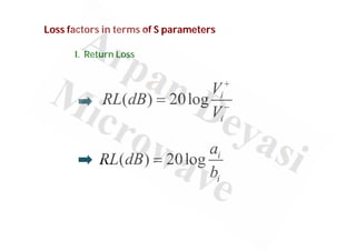
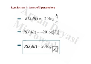
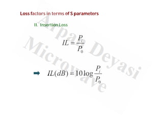
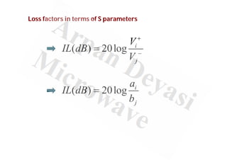
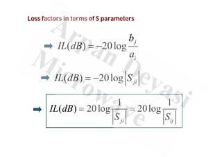
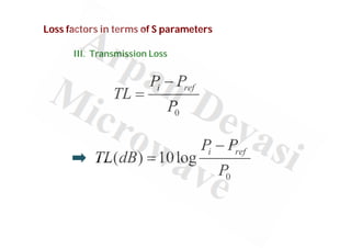
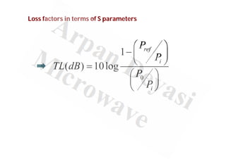
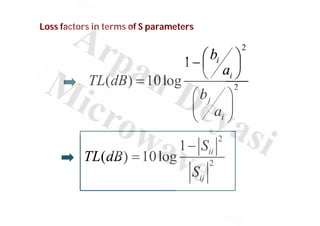
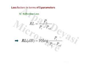
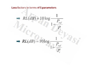
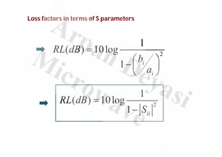

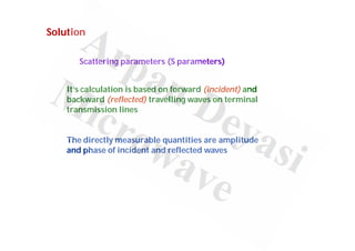
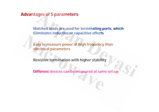
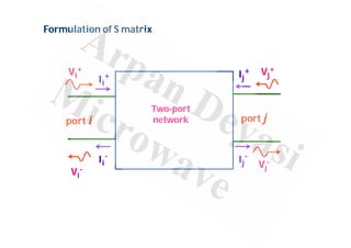
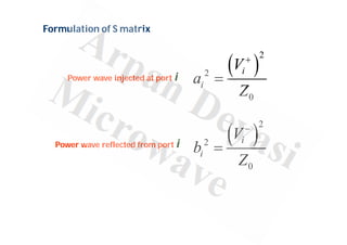
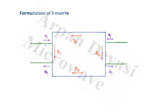
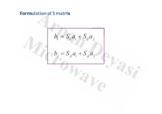
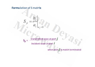
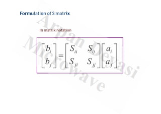
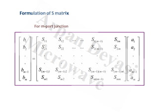
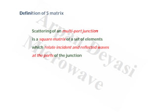
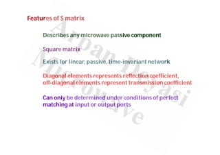
This document discusses scattering matrices (S-parameters) which relate the incoming and outgoing wave amplitudes at the ports of a network. It provides definitions and formulations for S-parameters, including that an S-matrix is a square matrix that describes the scattering properties of passive, linear, and time-invariant microwave networks. Key advantages of S-parameters are that matched loads are used, eliminating termination effects, and power can be easily measured at high frequencies. Loss factors like return loss, insertion loss, transmission loss, and reflection loss are also defined in terms of S-parameters.


![RF Circuit Design - [Ch3-1] Microwave Network](https://cdn.slidesharecdn.com/ss_thumbnails/ch3-1-150613064402-lva1-app6892-thumbnail.jpg?width=640&height=640&fit=bounds)


![RF Circuit Design - [Ch3-2] Power Waves and Power-Gain Expressions](https://cdn.slidesharecdn.com/ss_thumbnails/ch3-2-150613064404-lva1-app6891-thumbnail.jpg?width=640&height=640&fit=bounds)


![RF Circuit Design - [Ch1-2] Transmission Line Theory](https://cdn.slidesharecdn.com/ss_thumbnails/ch1-2-150613064349-lva1-app6892-thumbnail.jpg?width=640&height=640&fit=bounds)


