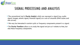
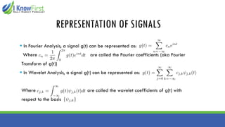
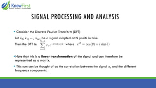
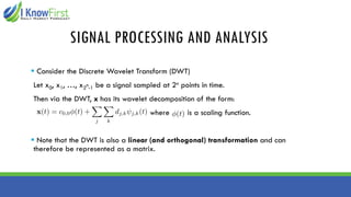
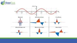
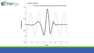
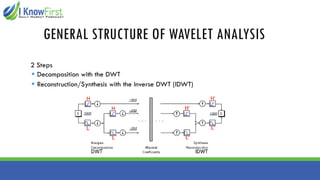
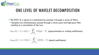
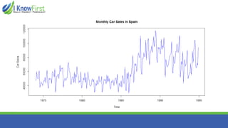
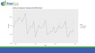
The document discusses wavelet analysis and its applications in various fields, including data compression, signal analysis, and financial markets. It compares wavelet analysis to traditional Fourier analysis, highlighting advantages such as the ability to capture both time and frequency information, particularly for signals with abrupt changes. Additionally, it presents a case study on forecasting car sales in Spain using wavelet analysis combined with ARIMA models, demonstrating improved accuracy in forecasts.

1. Wavelet Analysis
By Sam Luxenberg
23rd March 2017, Tel Aviv

2. INTRODUCTION TO WAVELETS
Applications:
▪ Data Compression
▪ Signal Analysis
▪ Smoothing/De-noising Data
▪ Modeling Abrupt Changes
▪ Pattern Recognition
▪ Solutions to Partial Differential Equations

3. WAVELETS AND FINANCIAL MARKETS
▪Markets are complex chaotic systems that have self-similarity properties.
▪Financial signals can be thought of as fractal signals having self-similarity properties
which allows for analysis with wavelets.

4. SIGNAL PROCESSING AND ANALYSIS
▪ The conventional tool is Fourier Analysis which can represent a signal (e.g. audio
signal, images, seismic signal, financial signal) as a sum of sinusoids (think cosine and
sine curves).
▪ We may be interested in certain cyclic or frequency components present in a signal.
▪ The Fourier Transform allows us to study the signal not just as it relates to time, but
also these frequency components.

5. REPRESENTATION OF SIGNALS
▪ In Fourier Analysis, a signal g(t) can be represented as:
Where are called the Fourier coefficients (aka Fourier
Transform of g(t))
▪ In Wavelet Analysis, a signal g(t) can be represented as:
Where are called the wavelet coefficients of g(t) with
respect to the basis

6. SIGNAL PROCESSING AND ANALYSIS
▪ Consider the Discrete Fourier Transform (DFT)
Let x0, x1, …, xN-1 be a signal sampled at N points in time.
Then the DFT is: where
▪Note that this is a linear transformation of the signal and can therefore be
represented as a matrix.
▪ This sum can be thought of as the correlation between the signal xn and the different
frequency components.

7. SIGNAL PROCESSING AND ANALYSIS
▪ Consider the Discrete Wavelet Transform (DWT)
Let x0, x1, …, x2n-1 be a signal sampled at 2n points in time.
Then via the DWT, x has its wavelet decomposition of the form:
where is a scaling function.
▪ Note that the DWT is also a linear (and orthogonal) transformation and can
therefore be represented as a matrix.

10. GENERAL STRUCTURE OF WAVELET ANALYSIS
2 Steps
▪ Decomposition with the DWT
▪ Reconstruction/Synthesis with the Inverse DWT (IDWT)

11. ONE LEVEL OF WAVELET DECOMPOSITION
▪ The DWT of a signal x is calculated by passing it through a series of filters.
▪ Samples are simultaneously passed through a lower-pass and high-pass filter
resulting in a convolution of the two.
▪ (approximation or scaling coefficients)
▪ (detail coefficients)

13. ADVANTAGES OVER FOURIER TRANSFORM
▪ Due to the Heisenberg Uncertainty Principle, we can study a signal with a Fourier
Transform with information in time or with information in frequency BUT NOT BOTH.
▪ E.g. We may know some frequency component occurs often throughout the existence
of a signal but we cannot know the timing this frequency occurs in the signal.
▪The two graphs below demonstrate the difference between examining a signal in the
time domain versus the frequency domain.

14. ADVANTAGES OVER THE FOURIER TRANSFORM

15. ADVANTAGES OVER THE FOURIER TRANSFORM
▪ The Wavelet Transform allows us to get both time and scale (the analogue for
frequency for wavelets) information simultaneously.
▪ J represents the “scale” or the “resolution level” at which we would want to examine
the signal.
▪ K represents the “translation” or “shift” in time.

16. ADVANTAGES OVER THE FOURIER TRANSFORM
▪ The Fourier Transform does NOT represent abrupt changes efficiently
▪ To accurately analyze signals and images with abrupt changes, use the wavelet
transform which is localized in time and frequency

17. WAVELET ANALYSIS AND TIME SERIES
“Time Series Forecasts Via Wavelets: An Application to Car Sales in the Spanish
Market” by Miguel Ariño, Ph.D.

18. GENERAL OUTLINE
▪ We will first forecast the time series using conventional time series modeling tools
such as Autoregressive Integrated Moving Average (ARIMA) and Seasonal ARIMA
(SARIMA).
▪ We want to compare the accuracy of these forecasts to forecasts combining wavelet
analysis and ARIMA models.

19. COMBINING WAVELET ANALYSIS AND ARIMA
▪ Decompose the time series into its long-term trend and seasonal component using
wavelet decomposition and reconstruction.
▪ Using ARIMA models, forecast each component separately.
▪ Combine these forecasted components to get the forecast for the original time series.

20. DATA
▪ Monthly Car Sales in Spain from January 1974 to December 1994.
▪ 252 total observations
▪ We will use the first 240 observations to build the models and the last 12 to
compare our forecasts with the actual number of sales during 1994.

22. ARIMA MODELS
▪ There are general rules of thumb to follow when identifying ARIMA models.
▪ Examine the Autocorrelation (correlation between each observation and the past
observations) and Partial Autocorrelation (correlation not accounted for by lags in-
between)
▪ Take differences (if necessary) to remove non-stationarity of the time series
▪ Two good models describe our time series:
▪ ARIMA(0, 1, 1)x(0, 1, 1)12
▪ ARIMA(2, 1, 0)x(0, 1, 1)12

23. ARIMA (0, 1, 1) X (0, 1, 1)12
▪ While both models give similar forecasts, the first model is simpler so we will use this
one.
▪ No AR component, 1 non-seasonal difference, 1 moving average component
▪ No seasonal AR component, 1 seasonal difference, 1 seasonal moving average
component with seasonal frequency being 12 months
▪ The out-of-sample root mean square error (RMSE) is 16,963.9

25. WAVELET MODEL – PREPARING TO USE DWT
▪ In order to use the DWT, we need the number of data points to be a power of 2
▪ Center the time series by subtracting its mean 60,603
▪ This centered or zero-mean series is called x = (xt)
▪ Daubechies of order 8 Wavelet basis

26. WAVELET MODEL - DWT
▪ Apply DWT to our time series x to obtain another series or vector called d which will
represent our scaling and wavelet coefficients.
▪ The DWT can be represented as a matrix, so applying the DWT can be thought of
as:
▪ For each level there will be associated coefficients

28. LONG-TERM TREND AND SEASONAL COMPONENT
▪ Scalogram is a graph of the amount of “energy” for each level of resolution to
identify the two most dominant resolution levels to use as the long-term trend and
seasonal components.
▪ For each resolution level and amount of shift/translation k
▪ Example for 2nd Resolution level:

30. SPLITTING THE COEFFICIENTS INTO 2 SETS
▪ There are two major peaks in the scalogram at levels 1 (7th decomposition) and 7
(1st decomposition).
▪ Existence of peaks at high or low levels indicates the existence of high or low
frequency components.
▪ Take coefficients at levels around each of the major peaks and pad each of these 2
coefficient vectors with zeros.

31. RECONSTRUCTION OF THE COMPONENTS
▪ Now that we have the 2 separate sets of coefficients, let’s reconstruct the individual
components using the IDWT.

32. BACK TO FORECASTING
▪ We have decomposed our time series into simpler and easier-to-forecast
components.
▪ In order to forecast y we need to add back in the mean of the original time series
that we subtracted before doing the wavelet analysis.
▪ Decomposition and Reconstruction on the boundary
▪ Delete first 36 and last 16 data points of each of our series x, y, and z.
▪ Left with car sales from January 1977 to December 1993

34. FORECASTING THE COMPONENTS
▪ Seasonality removed from the long-term trend y
▪ Best model for y: ARIMA(1,3,0)
▪ Seasonal model z
▪ Best model for z: ARIMA(0,1,1)12
▪ Forecasts for x
▪ x = y + z

36. COMPARISON OF THE MODELS
▪ Wavelet Model RMSE = 12,194
▪ SARIMA Model RMSE = 16,964

37. POTENTIAL APPLICATIONS FOR I KNOW FIRST
▪ Could provide more confidence to investment forecasts
▪ Overlay current forecasting systems on top of each of the decomposed wavelet
components.
▪ Wavelet analysis does not have to be constrained to 1-dimensional problems
▪Could be used for n-dimensional problems which could include considering an entire
portfolio of investments.

38. USEFUL RESOURCES
▪ Wavelet Toolbox User’s Guide
▪http://web.mit.edu/1.130/WebDocs/wavelet_ug.pdf
▪The Discrete Wavelet Transform in S
▪http://www.stat.ucla.edu/~cocteau/stat204/readings/nasonsilverman.pdf
▪Wavelet Scalograms and Their Applications in Economic Time Series
▪https://www.ime.usp.br/~pam/amv.pdf
▪“Conceptual Wavelets in Digital Signal Processing: An In-Depth, Practical Approach
for the Non-Mathematician” by D. Lee Fugal