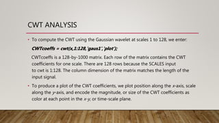
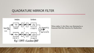
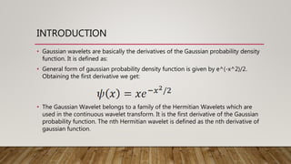
The Gaussian wavelet is defined as the derivative of the Gaussian probability density function. It belongs to a family of Hermitian wavelets used in continuous wavelet transforms. The nth Gaussian wavelet is the nth derivative of the Gaussian function. Gaussian wavelets have no scaling function and are not orthogonal or compactly supported, making the discrete wavelet transform and perfect reconstruction impossible. However, the continuous wavelet transform can be used to detect discontinuities in signals using Gaussian wavelets.

1. GAUSSIAN WAVELET
BY – MAHESH SAI CHAGANTI (2K19/SPDD/09)

2. INTRODUCTION
• Gaussian wavelets are basically the derivatives of the Gaussian probability density
function. It is defined as:
• General form of gaussian probability density function is given by e^(-x^2)/2.
Obtaining the first derivative we get:
• The Gaussian Wavelet belongs to a family of the Hermitian Wavelets which are
used in the continuous wavelet transform. It is the first derivative of the Gaussian
probability function. The nth Hermitian wavelet is defined as the nth derivative of
gaussian function.

3. PROPERTIES
• gaus(x,n) = Cn * diff(exp(-x^2),n) where diff denotes the symbolic derivative and
where Cn is a constant
• Orthogonal no
• Biorthogonal no
• Compact support no
• DWT no
• CWT possible

4. PROPERTIES

5. PROPERTIES
• Since Gaussian function is perfectly local in both time and frequency domain and
is infinitely derivable, so derivative of any order n of Gaussian function may be a
wavelet.

6. PROPERTIES
Fourier transform of Gaussian wavelet is:
When compared with Gaussian wavelet in time domain i.e.
We see that both have the same shape. The difference between both of them is
only a constant.

7. PROPERTIES
This figure graphically shows
Gaussian wavelet and its
transform

8. WAVELET ADMISSIBILITY CONDITION
• Regardless of its scale and magnitude, a function ψ is admissible as a wavelet if
and only if
• for which it is sufficient that its mean vanish or zero-mean condition:
• Since H(0)=0 for Gaussian wavelet i.e. ∫h(t)dt=0. So the wavelet admissibility
condition is satisfied.

9. GAUSSIAN WAVELET IN MATLAB
• [psi,x] = gauswavf(lb,ub,n,1);
• Where lb and ub represent lower and upper boundaries(grid parameters)
respectively.
• ‘n’ represents effective support width
• 1 is the order of the gaussian wavelet.
• Psi-wavelet function
• Gaussian wavelet has no scaling function(phi)

10. INTERPRETING WAVELET COEFFICIENTS
• CWT coefficients depend on the wavelet.
• A signal feature that wavelets are very good at detecting is a
discontinuity or singularity.
• Abrupt transitions in signal result in wavelet coefficients with large
absolute values.

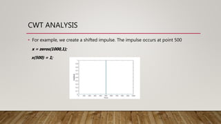
11. CWT COEFFICIENTS
• Assume that you have a wavelet supported on [-C, C]. Shifting the wavelet by b and scaling
by a results in a wavelet supported on [Ca+b, Ca+b].
• For the simple case of a shifted impulse, δ(t−τ), the CWT coefficients are only nonzero in
an interval around τ equal to the support of the wavelet at each scale.
• For the impulse, the CWT coefficients are equal to the conjugated, time-reversed, and
scaled wavelet as a function of the shift parameter, b

12. CWT ANALYSIS
• For example, we create a shifted impulse. The impulse occurs at point 500
x = zeros(1000,1);
x(500) = 1;

13. CWT ANALYSIS
• To compute the CWT using the Gaussian wavelet at scales 1 to 128, we enter:
CWTcoeffs = cwt(x,1:128,’gaus1’,’plot’);
CWTcoeffs is a 128-by-1000 matrix. Each row of the matrix contains the CWT
coefficients for one scale. There are 128 rows because the SCALES input
to cwt is 1:128. The column dimension of the matrix matches the length of the
input signal.
• To produce a plot of the CWT coefficients, we plot position along the x-axis, scale
along the y-axis, and encode the magnitude, or size of the CWT coefficients as
color at each point in the x-y, or time-scale plane.

16. CWT ANALYSIS
• Examining the CWT of the shifted impulse signal, we can see that the set of large
CWT coefficients is concentrated in a narrow region in the time-scale plane at
small scales centered around point 500. As the scale increases, the set of large
CWT coefficients becomes wider, but remains centered around point 500.
• CWT coefficients became large in the vicinity of an abrupt change in the signal.
This ability to detect discontinuities is a strength of the wavelet transform.
• The preceding example also demonstrated that the CWT coefficients localize the
discontinuity best at small scales. At small scales, the small support of the wavelet
ensures that the singularity only affects a small set of wavelet coefficients

17. DWT ANALYSIS
• Requirement for perfect reconstruction:
• Most constructions of DWT make use of MRA which defines
wavelet by a scaling function.
Multi Resolution analysis is a design method of most of the
practically relevant DWTs.

18. DWT ANALYSIS
• In case of Gaussian wavelet, no such scaling function exists, so perfect
reconstruction is not possible.
• However both DWT and Inverse DWT of Gaussian wavelet can be implemeted
using Quadrature Mirror Filter(QMF) bank which approximates Gaussian function.
• Although a truly lossless QMF DWT is still an area of research.

19. QUADRATURE MIRROR FILTER
• A quadrature mirror filter is a filter whose magnitude response is the mirror
image of that of another filter with respect to quadrature frequency /2 .
Together these filters are known as the Quadrature Mirror Filter pair.
• It is often used to implement a filter bank that splits an input signal into two
bands. The resulting high-pass and low-pass signals are often reduced by a factor
of 2, giving a critically sampled two-channel representation of the original signal

20. QMF INTRO
The main stress of most of the researchers while designing filters for the QMF bank
has been on the elimination orminimization of the three distortions to obtain a
perfect reconstruction (PR) or nearly perfect reconstruction (NPR) system
The PR condition is:

23. QUADRATURE MIRROR FILTER
When alpha=2, this filter was illustrated as a
Gaussian Bell-like function by Daubechies

24. APPLICATIONS
• Mostly used in sharply transitioning parts of signals, which contain the richest
information.
• Biomedical signals like Heart-rate and ECG analyses especially to detect
arrhythmia(heart rate being either too slow or high).
• Vibration transients detection like earthquakes damage detection,etc.
• Internet traffic analysis

25. LIMITATIONS
• Gaussian wavelets have fixed mother wavelets, thus the time-frequency
waveforms are identical in form so it can be a hindrance in providing variety of
gains and resolutions.
• Gaussian wavelets do not have applicable fast algorithms. It is computationally
intensive.
• High redundancy is present in the coefficients at high scales.
• Only approximate reconstruction is possible.