This document provides an overview of adaptive filters, including: - Adaptive filters have coefficients that are adjusted based on input data to optimize performance, unlike fixed filters. - The LMS algorithm is commonly used to adjust coefficients to minimize the mean square error between the filter output and a desired signal. - Key applications of adaptive filters include noise cancellation, system identification, channel equalization, and echo cancellation.

1. E E 315
T
Adaptive Filter
Vol-7
A.H.M. Asadul Huq, Ph.D.
http://asadul.drivehq.com/students.htm
asadul.huq@ulab.edu.bd
02/03/13 15:14 A.H. 1

2. Adaptive Digital Filter
References
1. Digital Signal Processing Principles … 4/e – John G.
Proakis et al.
2. Adaptive filter theory – Simon Haykin
3. Adaptive Filters Theory and Applications – B.
Farhang-Boroujeny
4. Digital Signal Processing A practical Approach –
Emmanuel C. Ifeachor (P 645 – 680, 2/e)
02/03/13 15:14 A.H. 2

3. Fixed versus Adaptive Filter Design
Fixed
w0, w1, w2, …, wN-1
Determine the values of the coefficients of the digital filter
that meet the desired specifications and the values are
not changed once they are implemented.
Adaptive
W0(n), w1(n), w2(n), …, wN-1(n)
The coefficient values are not fixed. They are adjusted to
optimize some measure of the filter performance using
incoming input data and error.
02/03/13 15:14 A.H. 3

4. Introduction to Adaptive Filter [Efea 541]
• An adaptive filter is a digital filter with self-
adjusting characteristics.
• It adapts, automatically, to changes in its
input signals.
• A variety of recursive algorithms have been
developed for the operation of adaptive
filters, e.g., LMS, RLS, etc.
02/03/13 15:14 A.H. 4

5. Continued … Introduction to the Adaptive Filter
[Far 2]
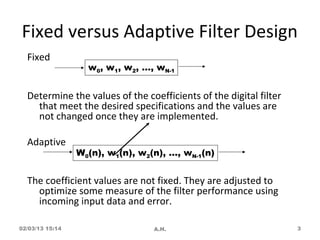
• The figure shows a filter emphasizing the way it is used in
typical problems.
• The filter is used to reshape certain input signals in such a
way that its output is a good estimate of the given desired
signal.
• The process of selecting or adapting in this case the filter
parameters (coefficients) so as to achieve the best match
between the desired signal and the filter output is often
done by optimizing an appropriately defined performance
function.
02/03/13 15:14 A.H. 5

6. Continued … Introduction to the Adaptive Filter
• The performance function can be defined in a statistical or
deterministic framework.
• In the statistical approach, the most commonly used performance
function is the mean-square value of the error signal, i.e. the
difference between the desired signal and the filter output. For
stationary input and desired signals, minimizing the mean-square
error results in the well-known Wiener filter, which is said to be
optimum in the mean-square sense.
• Most algorithms are practical solutions to Wiener filters.
• In the deterministic approach, the usual choice of performance
function is a weighted sum of the squared error signal. Minimizing
this function results in a filter which is optimum for the given set of
data.
• Depending on the certain statistical properties of the data, the
deterministic solution will approach the statistical solution, i.e. the
Wiener filter, for large data lengths.
02/03/13 15:14 A.H. 6

7. AF Classes
• Identification – The AF provides a model that
represents an unknown system.
• Inverse Modeling – The AF provides an inverse model
that represents an unknown system.
• Prediction – The AF provides the best prediction of
the present value of a random signal.
• Interference Canceling – The AF is used in such a way
that it can cancel unknown interference contained in
an information signal.
02/03/13 15:14 A.H. 7

8. Applications of AF
AF Classes Applications
Identification System Identification
Layered Earth Modeling
Inverse Modeling Adaptive equalization
Prediction ADPCM
Signal detection
Interference canceling Adaptive noise Canceling
Echo Cancellation
02/03/13 15:14 A.H. 8

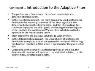
9. Adaptive Filter Structure [Far 3]
M −1
y (n) = ∑ wi (n) x(n − i )
i =0
02/03/13 15:14 A.H. 9

10. Continued .. Adaptive Filter Structure
• Adaptive filter is implemented using a transversal (FIR),
lattice or even IIR structure.
• FIR structure is the most widely used because of its
simplicity and guaranteed stability
• Where, the filter has input x(n) and an output, y(n). The
sequence d(n) is called the desired signal. wi(n)s are the
filter tap weights (coefficients) and M is the filter length.
The tap weights vary in time and are controlled by a
suitable adaptive algorithm.
• The output, y(n), is generated as a linear combination of the
delayed samples of the input sequence, x(n), according to
the equation - M −1
y (n) = ∑ wi (n) x(n − i )
i =0
02/03/13 15:14 A.H. 10

11. Adaptive Filter Algorithms [Ifea 648]
• LMS – Least Mean Square
• RLS – Recursive Least Squares
• Kalman Filter Algorithms
LMS
• The most efficient in terms of computation and storage
requirements
• Does not suffer from the numerical instability problem.
• Popular
02/03/13 15:14 A.H. 11

12. The LMS Algorithm
[Far 138, Ifea 654, Hay 299, Proa 902-905]
02/03/13 15:14 A.H. 12

13. Continued .. The LMS Algorithm
• The algorithm was derived by Widrow and Hoff in 1959
• The algorithm adapts each of the coefficient values of the tap vector
in the direction of the squared amplitude of the error signal
• Algorithm adaptation step size may be fixed to a suitable value.
• Input vector = {x(n)}=x(n), x(n-1) … x(n-M+1)
• Tap vector = {w(n)}=w0(n), w1(n), … wM-1(n)
where M-1 is the number of delay elements.
• Expected {w(n)} is computed using LMS algorithm.
• During the process of filtering, d(n) is supplied as the desired
response.
• Given the input vector, {x(n)}, and tap vector {w(n)}, the filter
produces an output y(n) which is an estimate of d(n).
• Now, calculate e(n)=d(n)-y(n)
02/03/13 15:14 A.H. 13

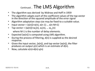
14. Continued .. The LMS Algorithm
We write here 3 basic relations of the LMS
algorithm [Hay 303, Far 141]
1. Filter output y ( n) = w T ( n) x ( n)
2. Estimation error e( n ) = d ( n ) − y ( n )
3. Tap-weight update w (n + 1) = w (n) + µx (n)e(n)
02/03/13 15:14 A.H. 14

15. Summary of the LMS Algorithm [Far 141]
02/03/13 15:14 A.H. 15

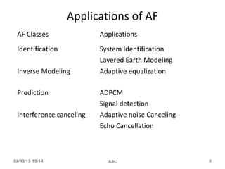
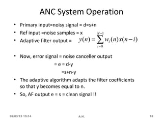
16. AF Application: Noise Cancellation
[Hay 48, Far 21, Proa 896]
• Adaptive Noise Cancelling (ANC) is performed by
subtracting noise from a signal (where noise has
been mixed) for the purpose of improved signal-
to-noise ratio.
• The filtering and subtraction are controlled by the
adaptive process.
• Basically an adaptive noise canceller is a dual
input, closed adaptive control system.
02/03/13 15:14 A.H. 16

17. Adaptive Noise Canceller (ANC)
Fig. (Proa 13.1.14) AF Canceller
02/03/13 15:14 A.H. 17

18. ANC System Operation
• Primary input=noisy signal = d=s+n
• Ref input =noise samples = x N −1
• Adaptive filter output = y ( n) = ∑ wi (n) x(n − i )
i =0
• Now, error signal = noise canceller output
= e = d-y
=s+n-y
• The adaptive algorithm adapts the filter coefficients
so that y becomes equal to n.
• So, AF output e = s = clean signal !!
02/03/13 15:14 A.H. 18

19. HOME WORKS
• Application of Adaptive filtering to system
identification(System Modeling) problem [Proa
P882].
• Adaptive Channel Equalization [Proa 883].
• Adaptive Echo Canellation [Proa 887].
02/03/13 15:14 A.H. 19

20. DSP Lecture
ADAPTIVE FILTER
THE END
THANK YOU
02/03/13 15:14 A.H. 20