Downloaded 965 times


![Flood Frequency Analysis
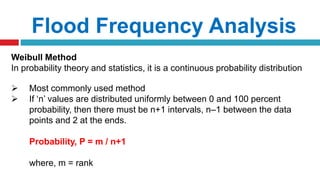
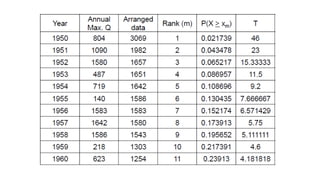
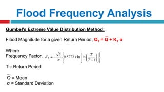
Gumbel’s Extreme Value Distribution Method:
E.J. Gumbel in 1941 was consider that annual flood peaks are extreme values of
floods in each of the annual series of recorded data. Hence, floods follow the
extreme value distribution.
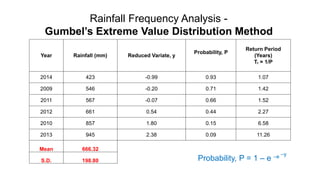
Probability, P = 1 – e –e –y
Return Period, T = 1/P
Where
y = reduced variate = [1.282 (Q – Q) / σ] + 0.577
e = base of Naperian Logarithm](https://image.slidesharecdn.com/wm-unitiii-160115174218/85/Runoff-Flood-Frequency-Analysis-52-320.jpg)
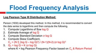
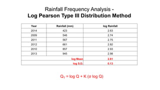

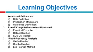
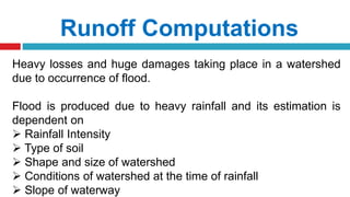
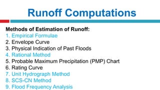
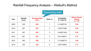
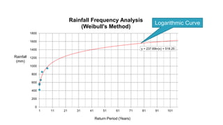
The document outlines methodologies for watershed management, including delineation, runoff computation, and flood frequency analysis. It describes various methods for estimating runoff, such as empirical formulae and the rational method, as well as techniques for flood frequency analysis, including the Weibull, Gumbel, and Log Pearson methods. Emphasis is placed on the significance of understanding watershed behavior and hydrological statistics in managing flood risks.