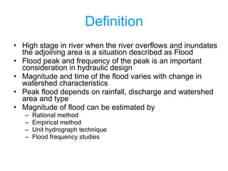
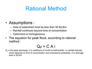
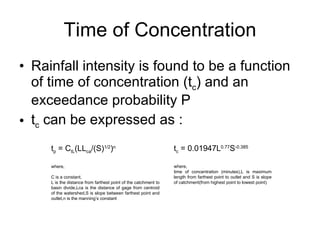
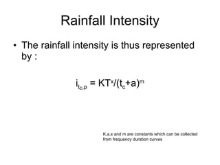
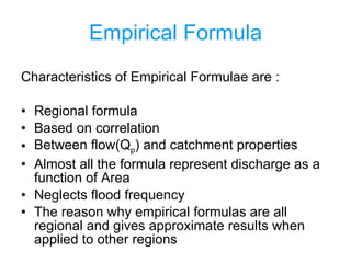
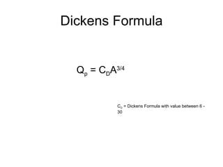
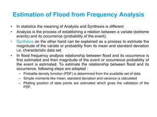
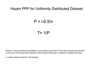
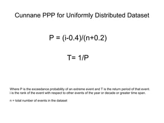
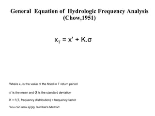
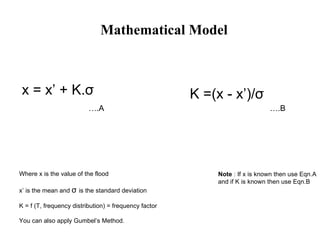
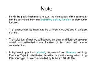
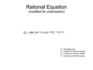
The document discusses various methods for estimating flood peaks, including the rational method, empirical formulas, unit hydrograph technique, and frequency analysis. It describes estimating time of concentration, rainfall intensity, and flood magnitude from watershed characteristics. Frequency analysis involves determining a probability density function from data, validating it using plotting positions, and estimating flood magnitudes for different return periods.

1. An Introduction to F L OO D Mrinmoy Majumder www.baipatra.ws

2. Definition High stage in river when the river overflows and inundates the adjoining area is a situation described as Flood Flood peak and frequency of the peak is an important consideration in hydraulic design Magnitude and time of the flood varies with change in watershed characteristics Peak flood depends on rainfall, discharge and watershed area and type Magnitude of flood can be estimated by Rational method Empirical method Unit hydrograph technique Flood frequency studies

3. Rational Method Assumptions : Area of watershed must be less than 50 Sq.Km Rainfall continues beyond time of concentration Catchment is homogeneous The equation for peak flood, according to rational method : Q p = C A i Q p is the peak discharge, C is coefficient of runoff (runoff/rainfall), i is rainfall intensity which depends on time of concentration and exceedance probability, A is drainage area in Sq.Km

4. Time of Concentration Rainfall intensity is found to be a function of time of concentration (t c ) and an exceedance probability P t c can be expressed as : t p = C tL (LL ca /(S) 1/2 ) n where, C is a constant, L is the distance from farthest point of the catchment to basin divide,Lca is the distance of gage from centroid of the watershed,S is slope between farthest point and outlet,n is the manning’s constant t c = 0.01947L 0.77 S -0.385 where, time of concentration (minutes),L is maximum length from farthest point to outlet and S is slope of catchment(from highest point to lowest point)

5. Rainfall Intensity The rainfall intensity is thus represented by : i t c ,p = KT x /(t c +a) m K,a,x and m are constants which can be collected from frequency duration curves

6. Empirical Formula Characteristics of Empirical Formulae are : Regional formula Based on correlation Between flow(Q p ) and catchment properties Almost all the formula represent discharge as a function of Area Neglects flood frequency The reason why empirical formulas are all regional and gives approximate results when applied to other regions

7. Dickens Formula Q p = C D A 3/4 C D = Dickens Formula with value between 6 - 30

8. Ryves Formula Q p = C R A 2/3 C R = Ryves Formula with value between 6.8 – 10.2

9. Inglis Formula Q p = (124A)/(A+10.4) 1/2 For Western Ghats in Maharashtra

10. Fullers Formula Q Tp = (C f A 0.8 )/(1+0.8logT) For USA,T = return period, C f is a constant =0.18 – 1.88.

11. Baird and Mcillwraith(1951) Q mp = (3025A)/(278+A) 0.78 From maximum rrecorded floods throughout the world

12. Estimation of Flood from Frequency Analysis In statistics the meaning of Analysis and Synthesis is different Analysis is the process of establishing a relation between a variate (extreme events) and its occurrence (probability of the event). Synthesis on the other hand can be explained as a process to estimate the magnitude of the variate or probability from its mean and standard deviation i.e. characteristic data set. In flood frequency analysis relationship between flood and its occurrence is first estimated and then magnitude of the event or occurrence probability of the event is estimated. To estimate the relationship between flood and its occurrence, following steps are adopted : Probable density function (PDF) is determined from the available set of data Simple moments like mean, standard deviation and variance is calculated Plotting position of data points are estimated which gives the validation of the PDF.

13. Analysis .Step.1 : Probability Density Function

14. Gumbels Method Where the distribution has mode α , mean α + γβ (where γ =0.5772156649... is Euler's constant ), and variance ⅙ β 2π2 If f(x) is probability density function, then, Gumbel’s distribution is given by :

15. Gumbel’s Distribution Explained There are essentially three types of Fisher-Tippett extreme value distributions. The most common is the type I distribution, which are sometimes referred to as Gumbel types or just Gumbel distributions. The term "Gumbel distribution" is used to refer to the distribution corresponding to a minimum extreme value distribution (i.e., the distribution of the minimum ). The Gumbel distribution has a location parameter α and scale parameter β

16. Normal Distribution = variate = mean = variance P(x) and D(x) is respectively the probability density function and distribution function

17. Log-Normal Distribution Normal distribution of the Logarithm of Variate. Mean and standard deviation is estimated with the help of logarithm of the variates. The probable density function and distribution function is adjusted accordingly.

18. Pearson Type III Distribution = gamma function = variate = mean = = variance = P(x) and Φ (t) is respectively the probability density function and characteristic function = kurtosis = = kurtosis =

19. Log-Pearson Distribution Pearson distribution of the Logarithm of the Variates. Mean and standard deviation is estimated with the help of logarithm of the variates. The probable density function is adjusted accordingly.

20. Analysis.Step.2 : Validation of the PDF by Estimation of Plotting Position of the Event or Plotting Position Probability

21. Plotting Position Probability (PPP) P = m/(N+1) T= 1/P Where P is the probability of an extreme event and T is the return period of that event. P rn is the occurrence of the event for r times in n successive years m is the rank of the event with respect to other events of the year or decade or greater time span. N = total number of events in the dataset C =combination of n and r and q = 1-P P rn = n C r P r q n-r T= 1/P

22. Bulletin 17B PPP (InterAgency Advisory Committee on Water Data,1982) P = (i-a)/(n-a-b+1) T= 1/P Where P is the exceedance probability of an extreme event and T is the return period of that event. i is the rank of the event with respect to other events of the year or decade or greater time span. n = total number of events in the dataset a and b are constants = f(PDF)

23. Weibull PPP for Uniformly Distributed Dataset P = i/(n+1) T= 1/P Where P is the exceedance probability of an extreme event and T is the return period of that event. i is the rank of the event with respect to other events of the year or decade or greater time span. n = total number of events in the dataset Uniformly distributed dataset means a = b = 0

24. Hazen PPP for Uniformly Distributed Dataset P = i-0.5/n T= 1/P Where P is the exceedance probability of an extreme event and T is the return period of that event. i is the rank of the event with respect to other events of the year or decade or greater time span. n = total number of events in the dataset

25. Cunnane PPP for Uniformly Distributed Dataset P = (i-0.4)/(n+0.2) T= 1/P Where P is the exceedance probability of an extreme event and T is the return period of that event. i is the rank of the event with respect to other events of the year or decade or greater time span. n = total number of events in the dataset

26. Synthesis i.e. Determination of the Magnitude

27. General Equation of Hydrologic Frequency Analysis (Chow,1951) x T = x ’ + K. σ Where x T is the value of the flood in T return period x’ is the mean and σ is the standard deviation K = f (T, frequency distribution) = frequency factor You can also apply Gumbel’s Method.

28. Mathematical Model x = x ’ + K. σ Where x is the value of the flood x’ is the mean and σ is the standard deviation K = f (T, frequency distribution) = frequency factor You can also apply Gumbel’s Method. K =(x - x ’)/ σ Note : If x is known then use Eqn.A and if K is known then use Eqn.B ….A ….B

29. Note If only the peak discharge is known, the distribution of the parameter can be estimated from the probability density function or distribution function. The function can be estimated by different methods and in different manner. The selection of method will depend on error or difference between actual and estimated curve, location of the basin and time of concentration. In hydrologic problems Normal , Log-normal and Pearson and Log-Pearson Type III distribution function is used among which Log-Pearson Type III is recommended by Bulletin 17B of USA.

30. Adjustment for Urbanization

31. Rational Equation (modified for urbanization) Q p = 484.1A 0.723 (1+U) 1.516 P E 1.113 T r 0.403 A = drainage area U = fraction of imperviousness P E = volume of excess rainfall T r = duration of rainfall excess

32. Adjustment for Urbanization Adjusted peak discharge due to observed impervious factor = Observed Peak Discharge multiplied by adjustment factor of the observed imperviousness

33. Urban Adjustment Factor (Leopold,1968)

34. Probable Maximum Precipitation PMP as the greatest depth of precipitation for a given duration that is meteorologically possible over a given station or a specified area. There are two major methods available to estimate value of PMP. The first is the meteorological method in which the PMP for different durations over an area is determined by transposition and maximisation of major historical rainstorms. The second is a statistical method where the estimates of PMP are derived from frequency analysis of the annual maximum rainfall series for different durations. The statistical method is useful when there is insufficient meteorological data to apply storm maximization method. A statistical method for estimating PMP for small areas has been developed by Hershfield , 1961 and Hershfield , 1965 based on a general frequency equation given by Chow (1951) .

35. Hershfield Method where X PMP is the PMP for a given station for a specific duration and X¯ n and σ n are the mean and standard deviation for a series of n annual maximum rainfall values of a given duration respectively. K m is the frequency factor and is the largest of all the calculated K values for all stations in a given area.

36. Frequency Factor Calculation where X 1 , X¯ n −1 and σ n −1 are the highest value, mean and standard deviation respectively excluding the X 1 value from the series.

37. Homogeneity of Dataset The use of a longer series in the estimation of PMP is appropriate only if they show no significant increasing or decreasing trends. The presence or absence of trends in the annual maximum rainfall series for the rainfall stations used were investigated using the Mann–Kendall rank statistics test ( WMO, 1966 ). the ratio of τ to the σ τ gives an indication of trend in the data. For no trend in the data series, this value should lie within the limits of ± 1.96 at the 5% level of significance.