This document defines key concepts and symbols used in hydrologic analysis for drainage design. It discusses hydrology as relating to estimating flood magnitudes from precipitation. Floods are considered in terms of peak runoff and hydrographs. The summary defines important concepts like antecedent moisture conditions, depression storage, frequency, hydraulic roughness, hydrographs, hyetographs, infiltration, interception, lag time, peak discharge, rainfall excess, stage, time of concentration, unit hydrograph. Symbols used in hydrologic analysis are also defined.


![Chapter 5
Hydrology Drainage Design Manual - 2002
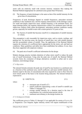
Time of Concentration
The time of concentration is the sum of T
t values for the various consecutive flow
segments:
T
c = T
t1 + T
t2 + … T
tm (5.8)
Where:
T
c = time of concentration, hr
m = number of flow segments.
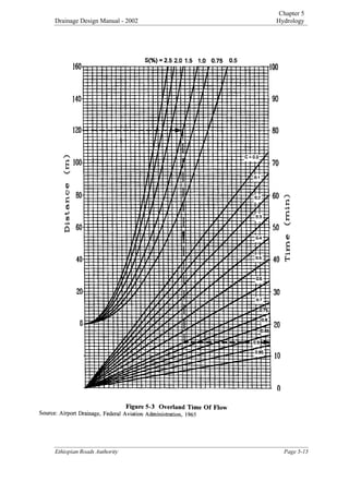
Sheet Flow
Sheet flow is flow over plane surfaces. It usually occurs in the headwater of streams.
With sheet flow, the friction value (Manning's n) is an effective roughness coefficient
that includes the effect of raindrop impact; drag over the plane surface; obstacles such as
litter, crop ridges, and rocks; and erosion and transportation of sediment. These n values
are for very shallow flow depths of about 0.03 m or so. Table 5-14 gives Manning's n
values for sheet flow for various surface conditions.
7DEOH5RXJKQHVVRHIILFLHQWV 0DQQLQJ¶VQ IRU6KHHW)ORZ
Surface Description
Smooth surfaces (concrete, asphalt, gravel, or bare soil
Fallow (no residue)
Cultivated soils:
Residue cover ≤ 20%
Residue cover 20%
Grasses:
Short grass
Dense Grasses
Range (natural)
Woods:
2
Light underbrush
Dense underbrush
n
1
0.011
0.05
0.06
0.17
0.15
0.24
0.13
0.40
0.80
1
The n values are a composite of information complied by Engman (1986).
2
When selecting n, consider cover to a height of about 0.03 m. This is the only part of the plant cover
that will obstruct sheet flow.
For sheet flow of less than 100 meters, use Manning's kinematic solution (Overton and
Meadows 1976) to compute T
t:
T
t = [0.091 (nL)
0.8
/ (P
2)
0.5
s
0.4
] (5.9)
Where:
T
t = travel time, hr
n = Manning's roughness coefficient (Table 5-14)
L = flow length, m
P
2 = 2-year, 24-hour rainfall, mm
s = slope of hydraulic grade line (land slope), m/m
3DJH (WKLRSLDQ5RDGV$XWKRULW](https://image.slidesharecdn.com/05-hydrology-231004074758-2bdad53e/85/Hydrology-pdf-30-320.jpg)
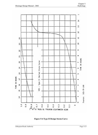
![Chapter 5
Hydrology Drainage Design Manual - 2002
Travel Time
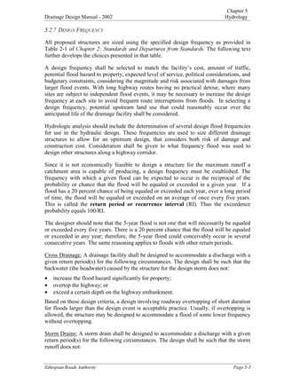
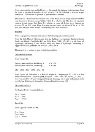
)LJXUHDWFKPHQW$UHD6HJPHQWV
For Segment A-B (see Figure 5-6): Sheet flow, natural range, slope = 0.10 m/m, length =
50m. From Table 5-14, Manning’s n = 0.13. The 2-year, 24-Hour rainfall is determined
from Figure 5-13 to be 65mm. From Equation 5.9,
T
t = [0.091 (nL)
0.8
/ (P
2)
0.5
s
0.4
] = 0.127 hr
For Segment B-C: Shallow concentrated flow, unpaved, s = 0.04 m/m, length = 500m.
From Equation 5.10:
V = 4.9178 (s)
0.5
= 0.984 m/s
From Equation 5.7:
T
t = L/(3600V) = 0.141 hr
For Segment C-D: channel flow, natural stream channel, winding with weeds and pools,
s = 0.01m/m, length = 2000m. From the survey, bottom width = 2m, sideslopes = 1V:1H,
25-year storm depth = 1m.
See Table 6-1 KDSWHUKDQQHOV: Manning’s n = 0.050.
A = Cross-sectional flow area = (2 x 1) + 2[1/2(1)] = 3m
2
P
w = wetted perimeter = 2m + 2¥ P
R = Hydraulic radius = A/P
w = 3/4.828 = 0.621m
From Equation 5.12
V = (r
2/3
s
1/2
)/n = 1.46 m/s. From Equation 5.7:
T
t = L/(3600V) = 0.381 hr
Total Time of Concentration = 0.127 + 0.141 + 0.381 = 0.649 hr
Peak Runoff
From the above data and calculations, catchment area = 100ha, Runoff Curve Number =
84, Time of Concentration = 0.649 hr, 25-year, 24-hour Storm, P = 118mm, Run-Off Q
25
= 81mm.
Determine Initial Abstraction from Table 5-15:
3DJH (WKLRSLDQ5RDGV$XWKRULW](https://image.slidesharecdn.com/05-hydrology-231004074758-2bdad53e/85/Hydrology-pdf-34-320.jpg)