Download as PDF, PPTX


The document provides definitions and concepts related to matrices and determinants. It begins with definitions of matrices, operations on matrices like transpose and trace. It then discusses row echelon form, elementary row operations, and using matrices to represent systems of linear equations. The document will cover topics like inverse matrices, matrix rank and nullity, polynomials of matrices, properties of determinants, minors and cofactors, and Cramer's rule.
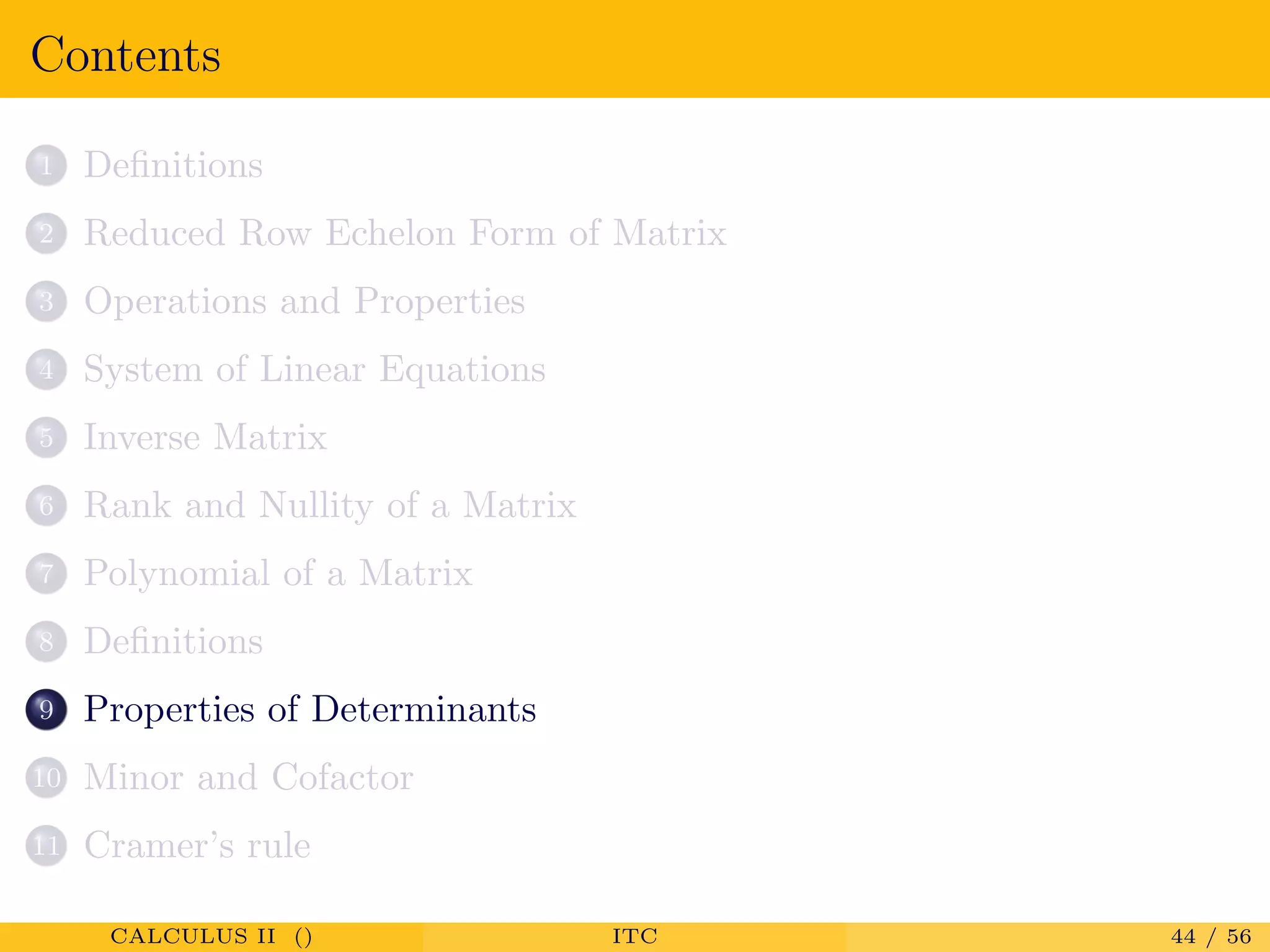
Introduction to matrices and determinants along with chapter contents for a calculus course.
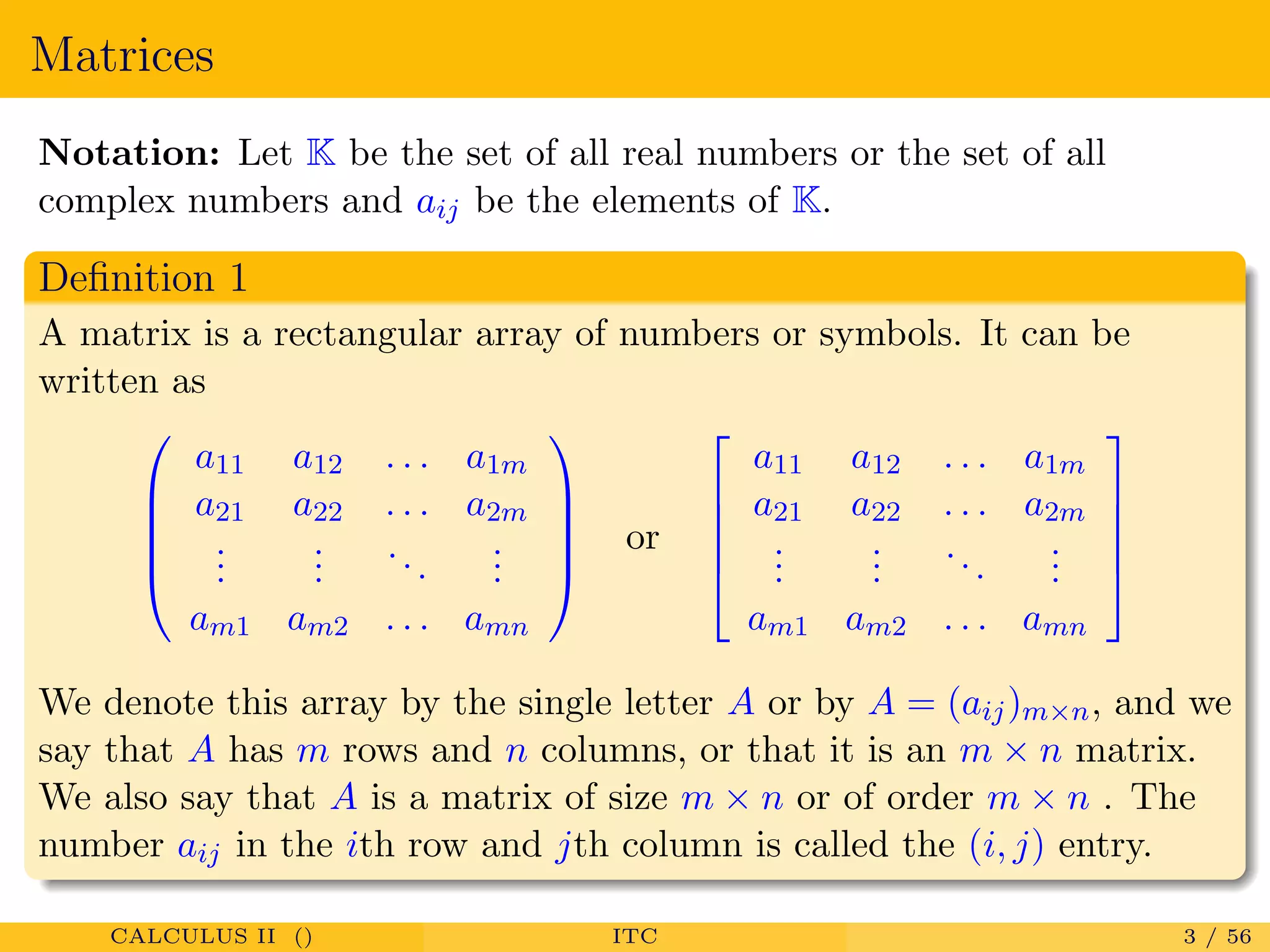
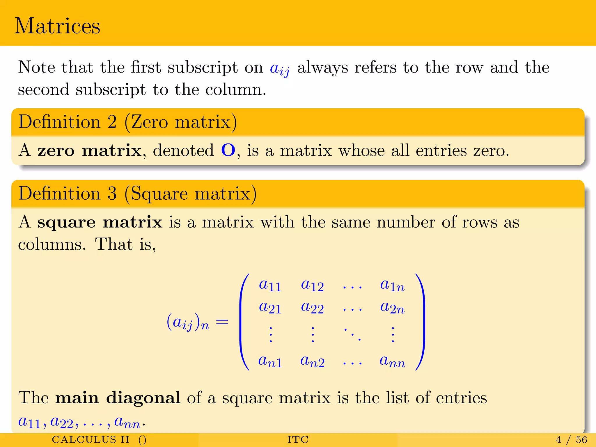
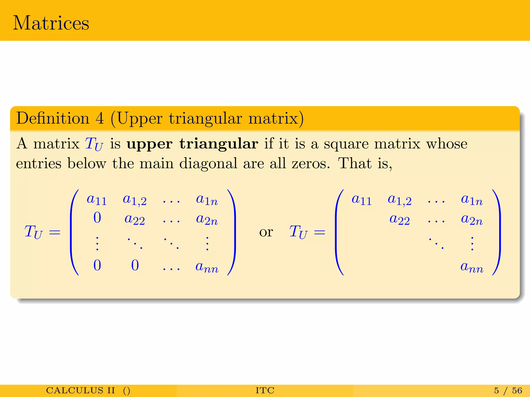
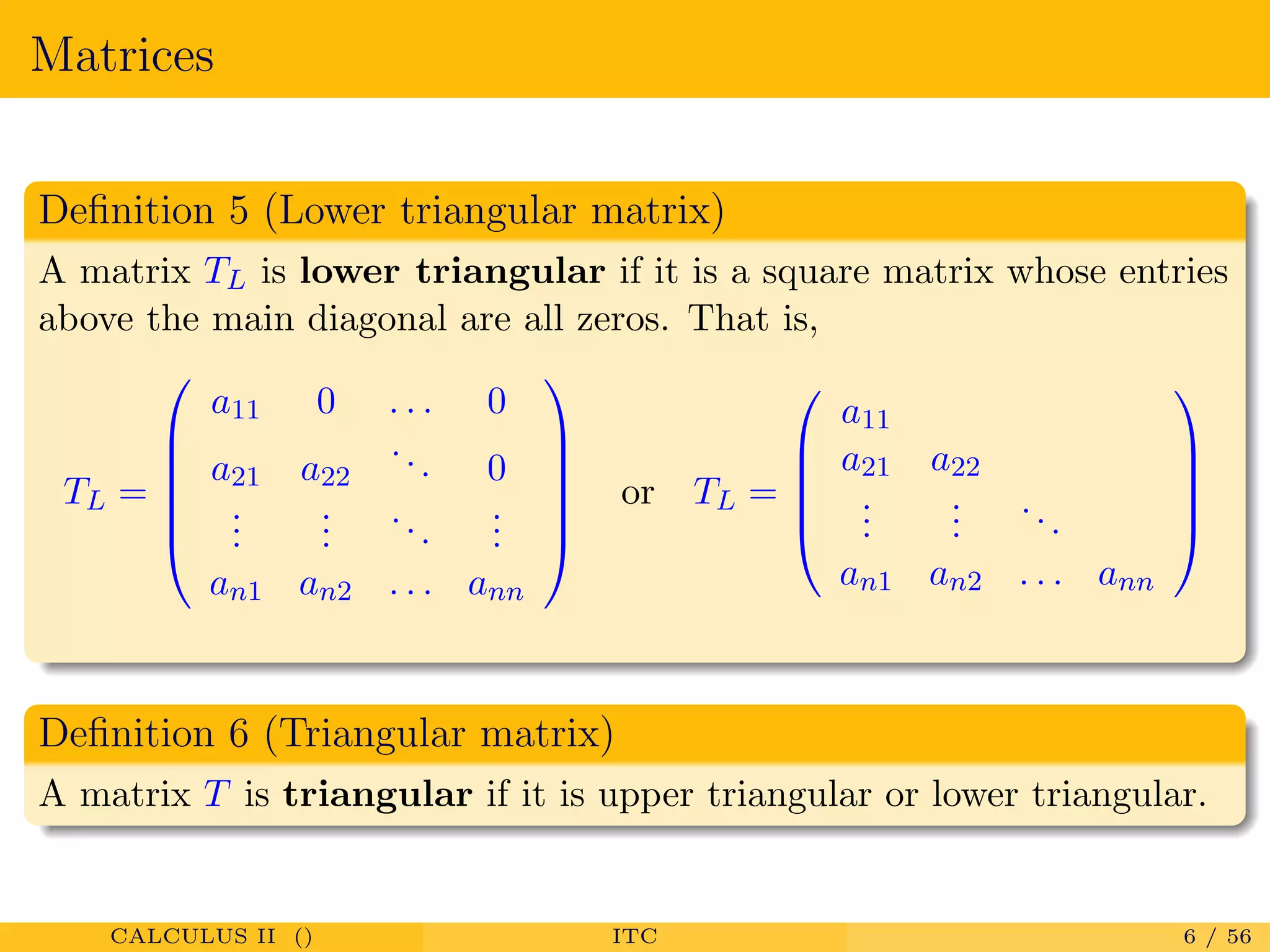
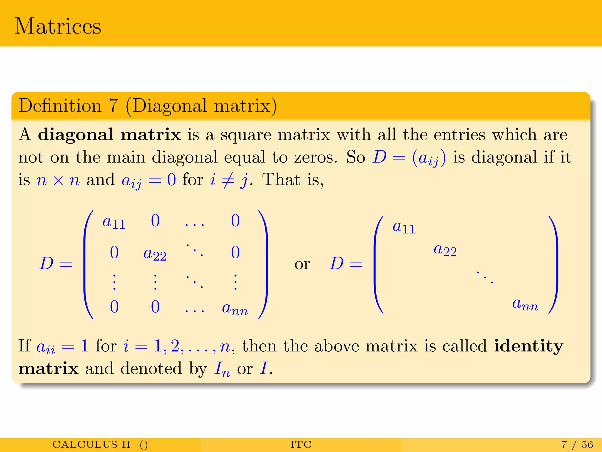
Definitions of matrix types including zero, square, upper/lower triangular, and diagonal matrices with their characteristics.
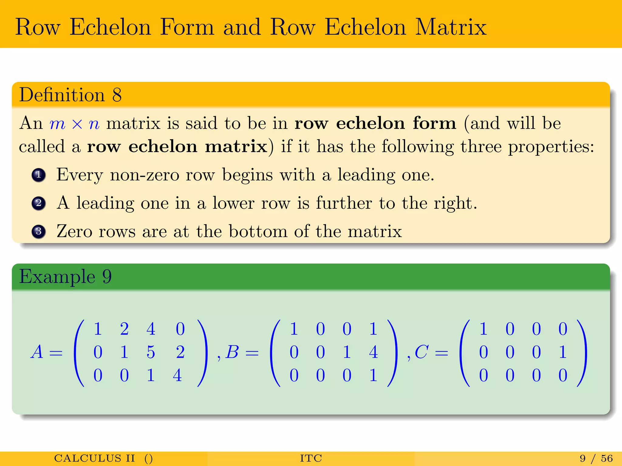
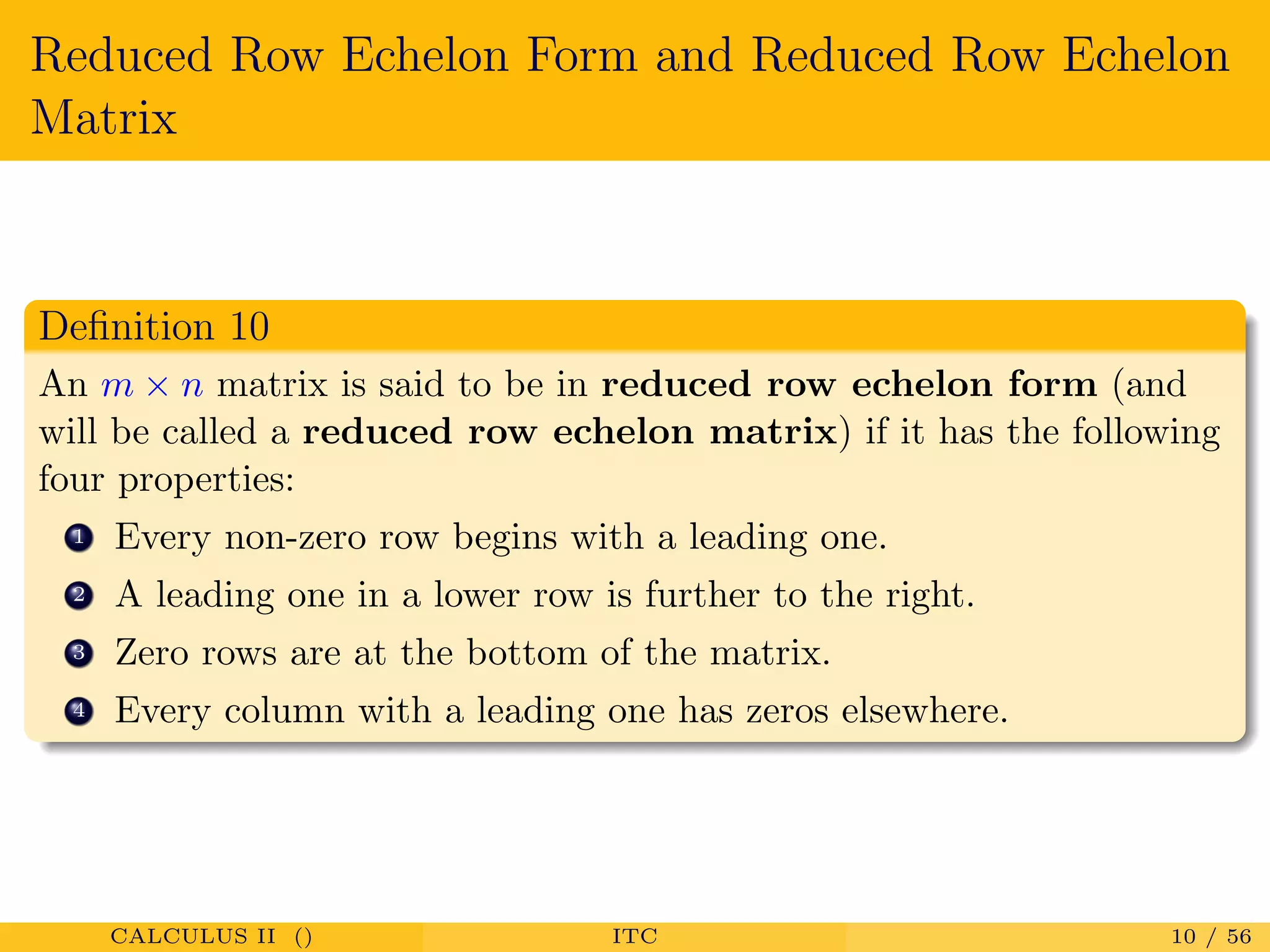
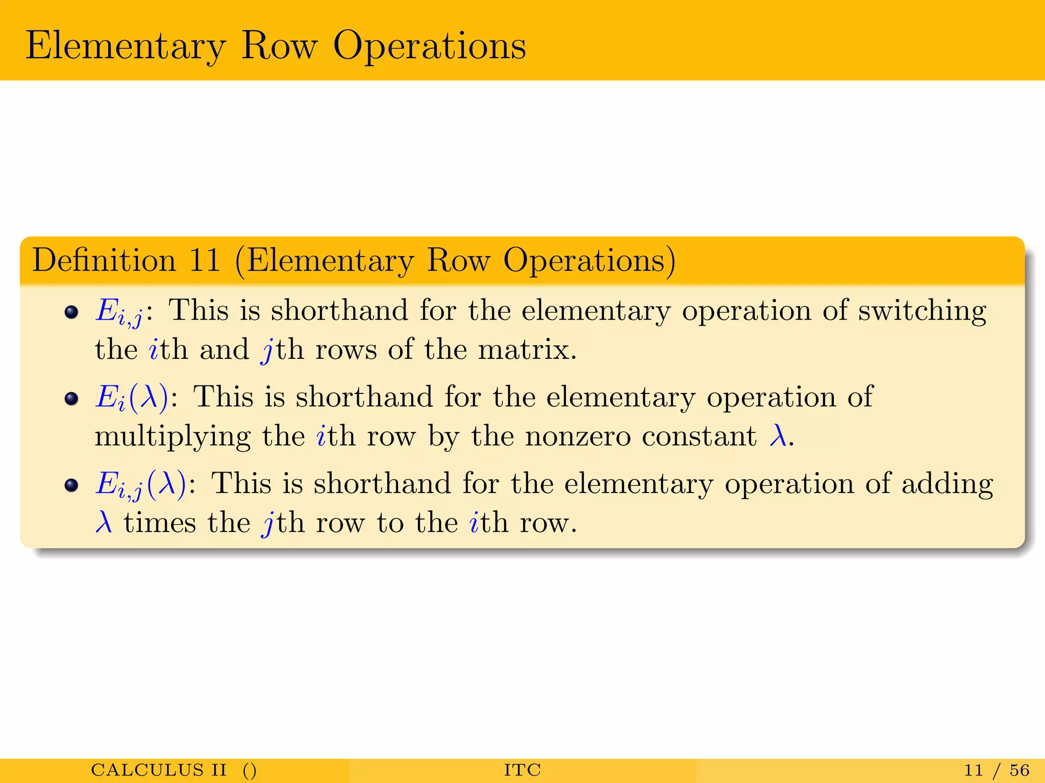
Introduction to row echelon forms and reduced row echelon forms, along with elementary row operations.
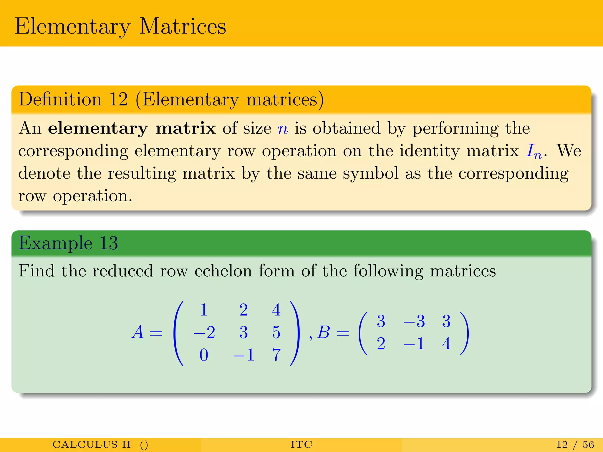
Definition of elementary matrices derived from row operations. Examples on finding reduced row echelon forms.
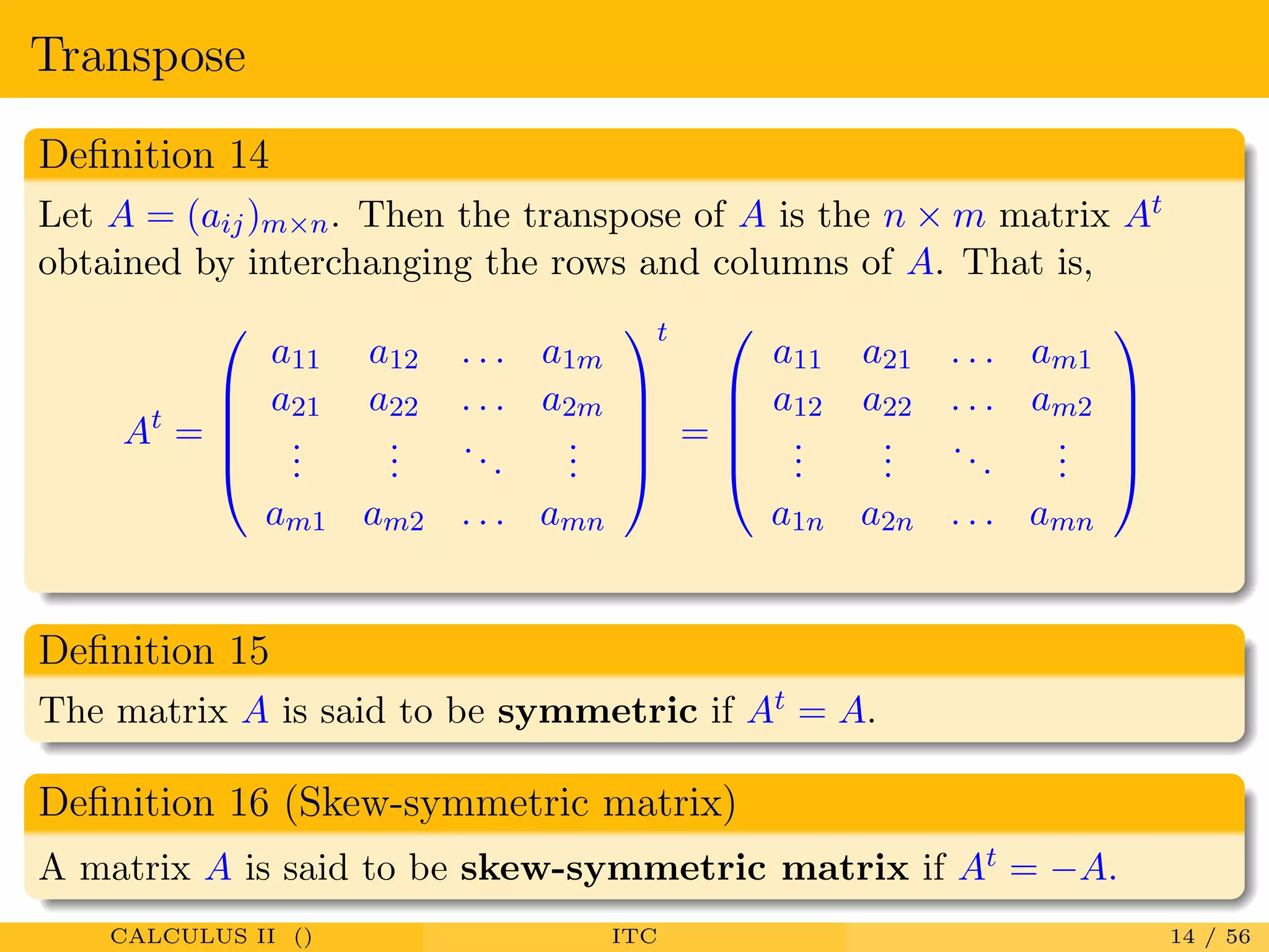
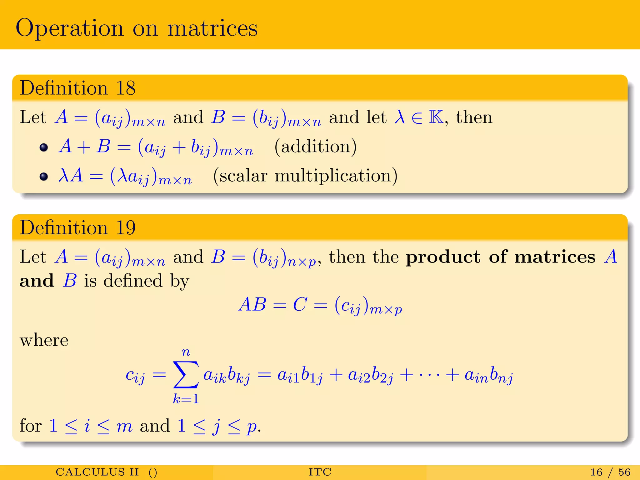
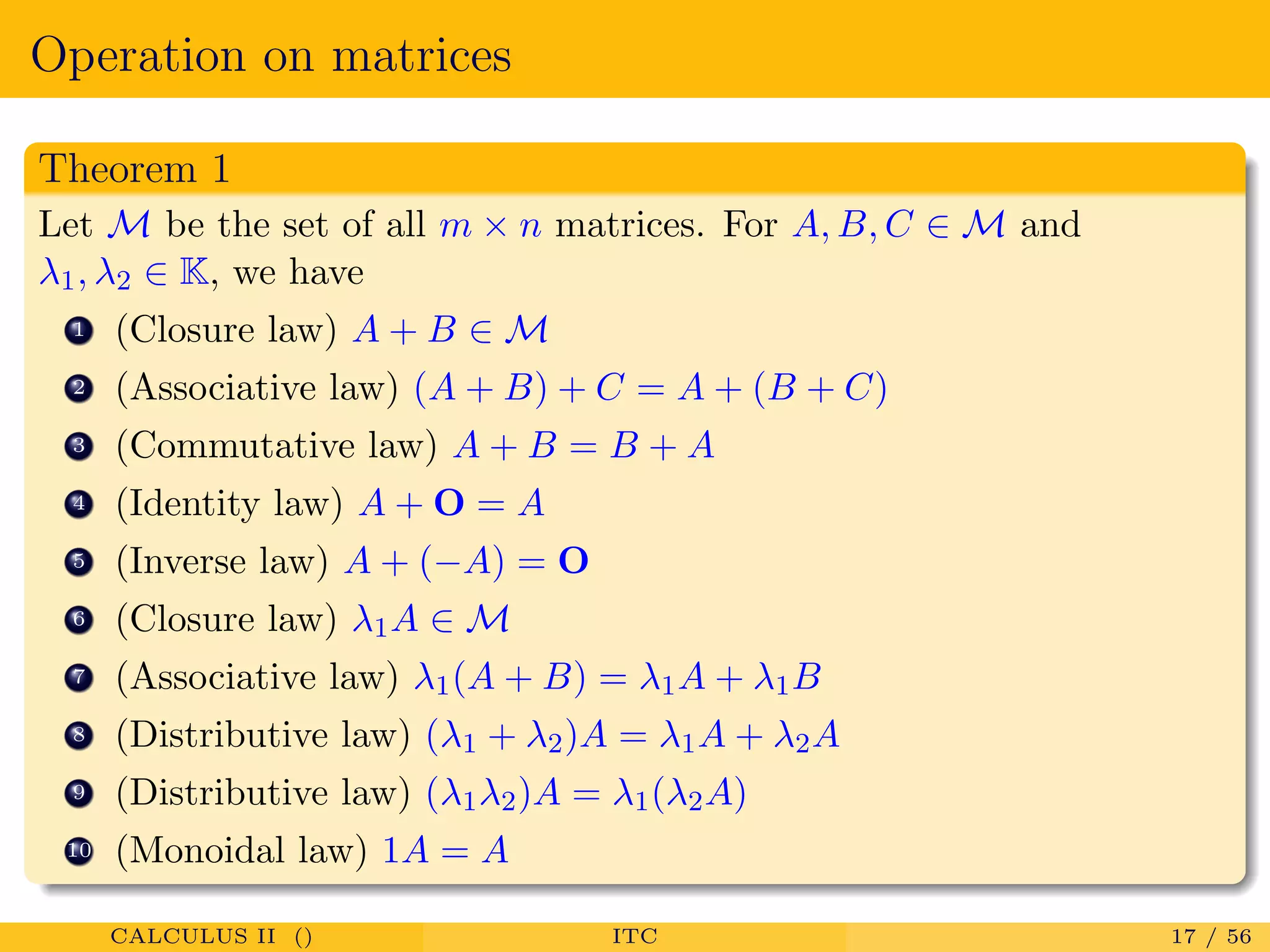
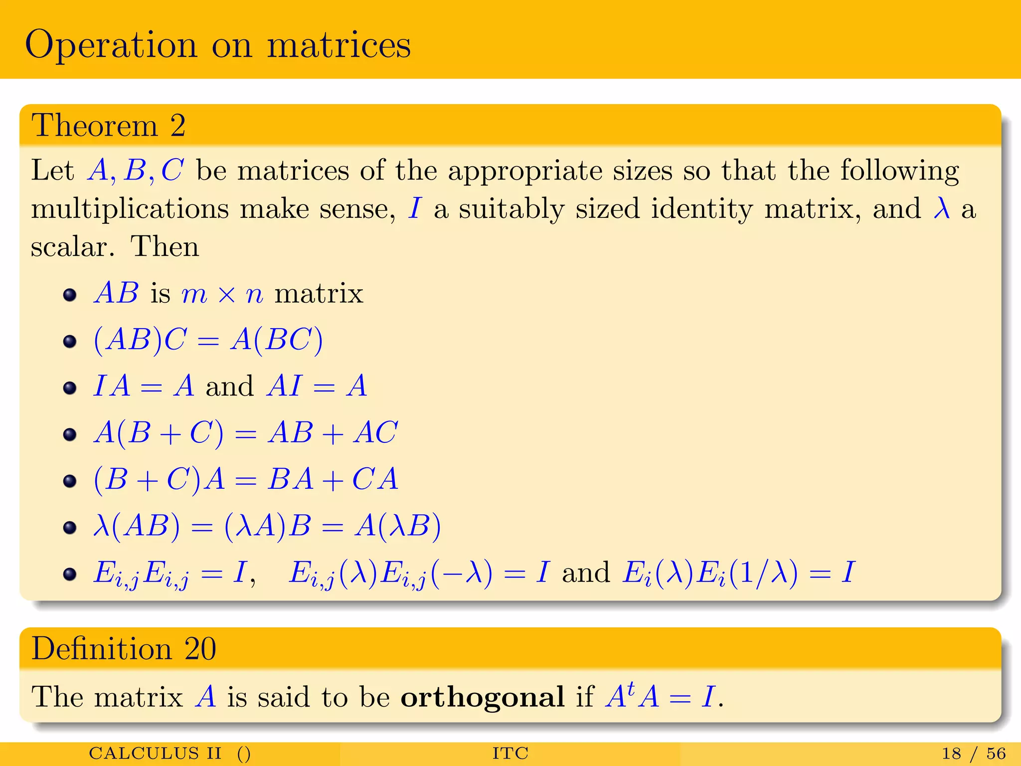
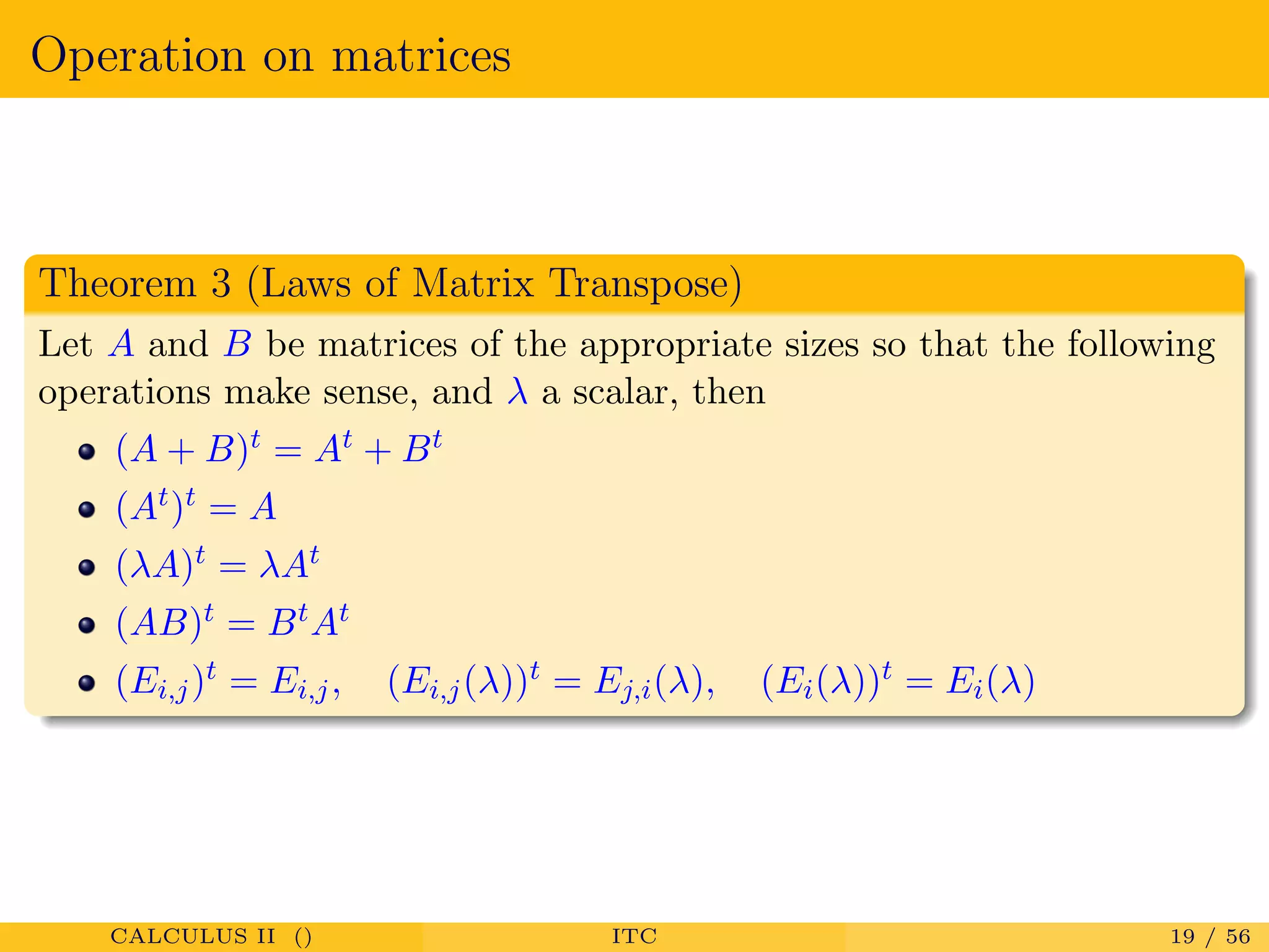
Definitions of transpose, symmetric, and skew-symmetric matrices and properties of matrix operations.
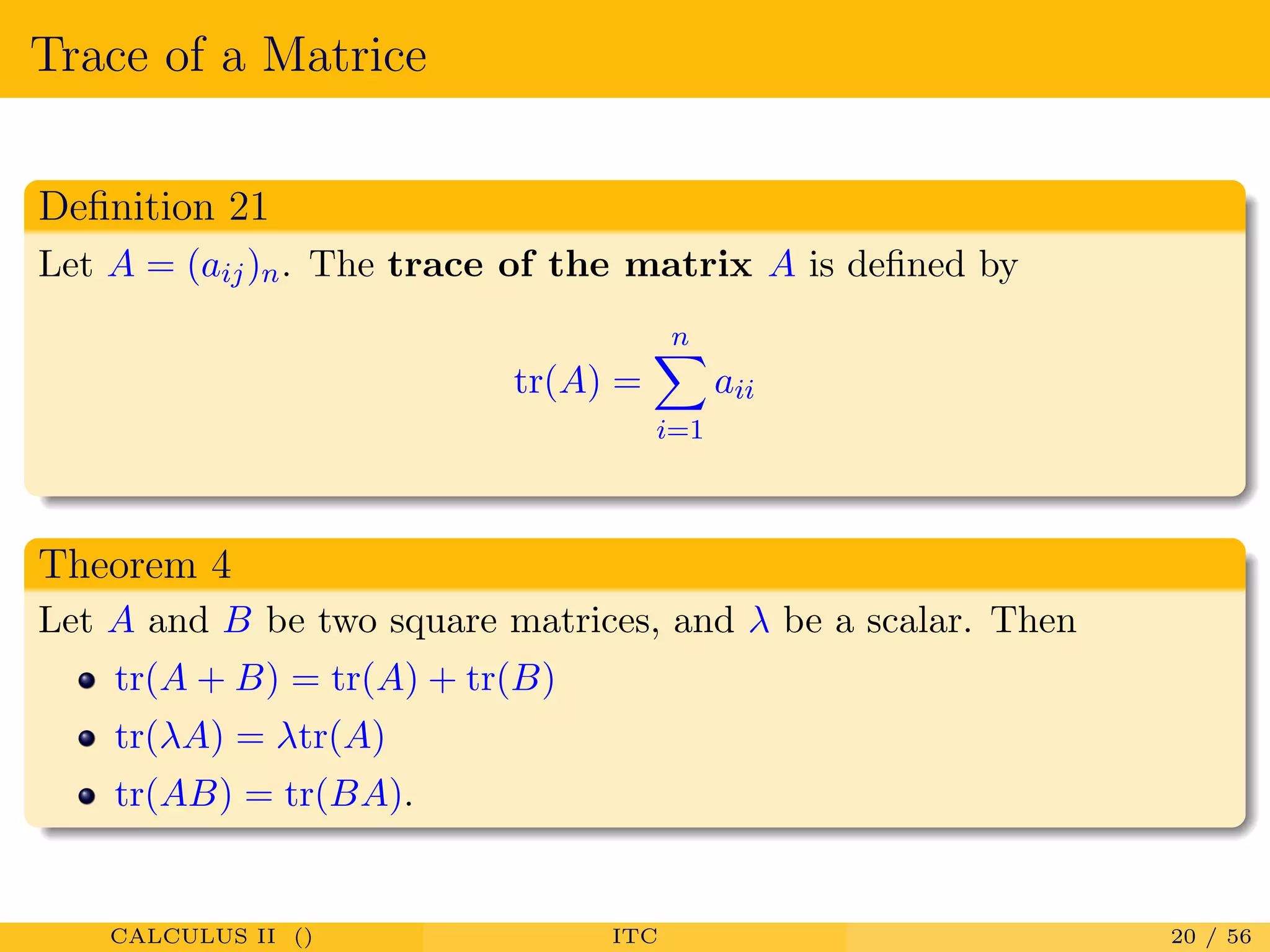
Definition of trace, a key feature of square matrices with its related properties.
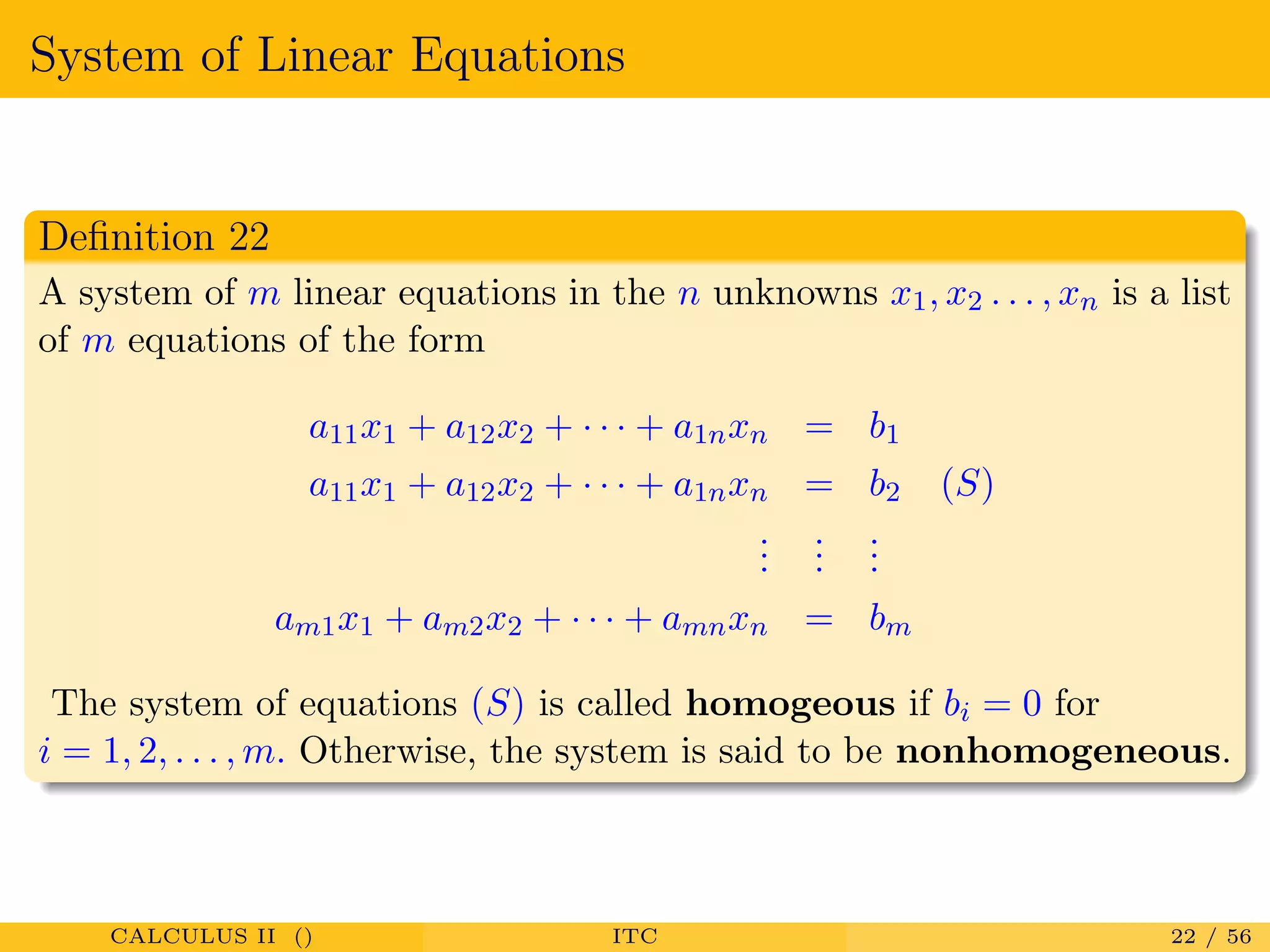
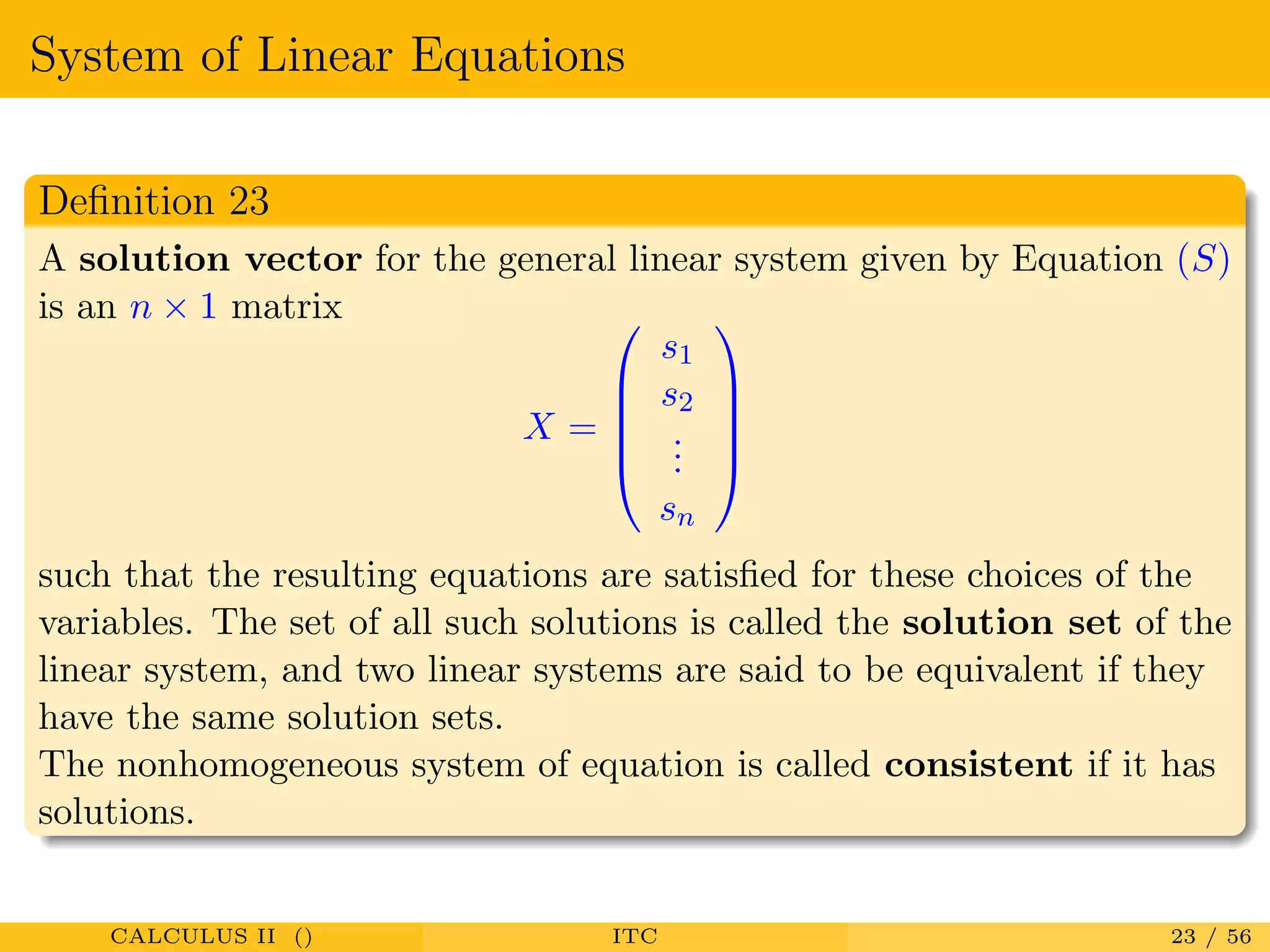
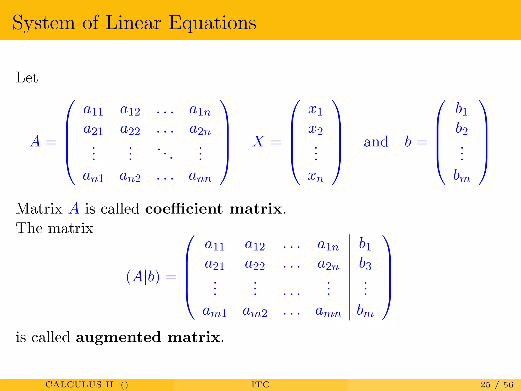
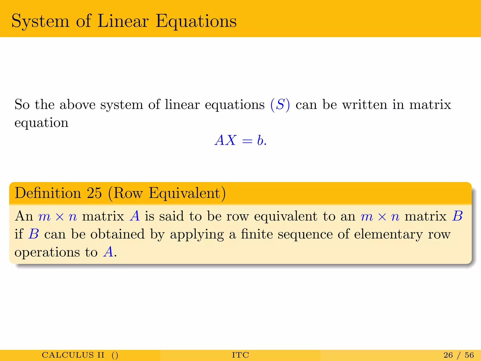
Defining systems of linear equations, distinguishing between homogeneous and nonhomogeneous systems.
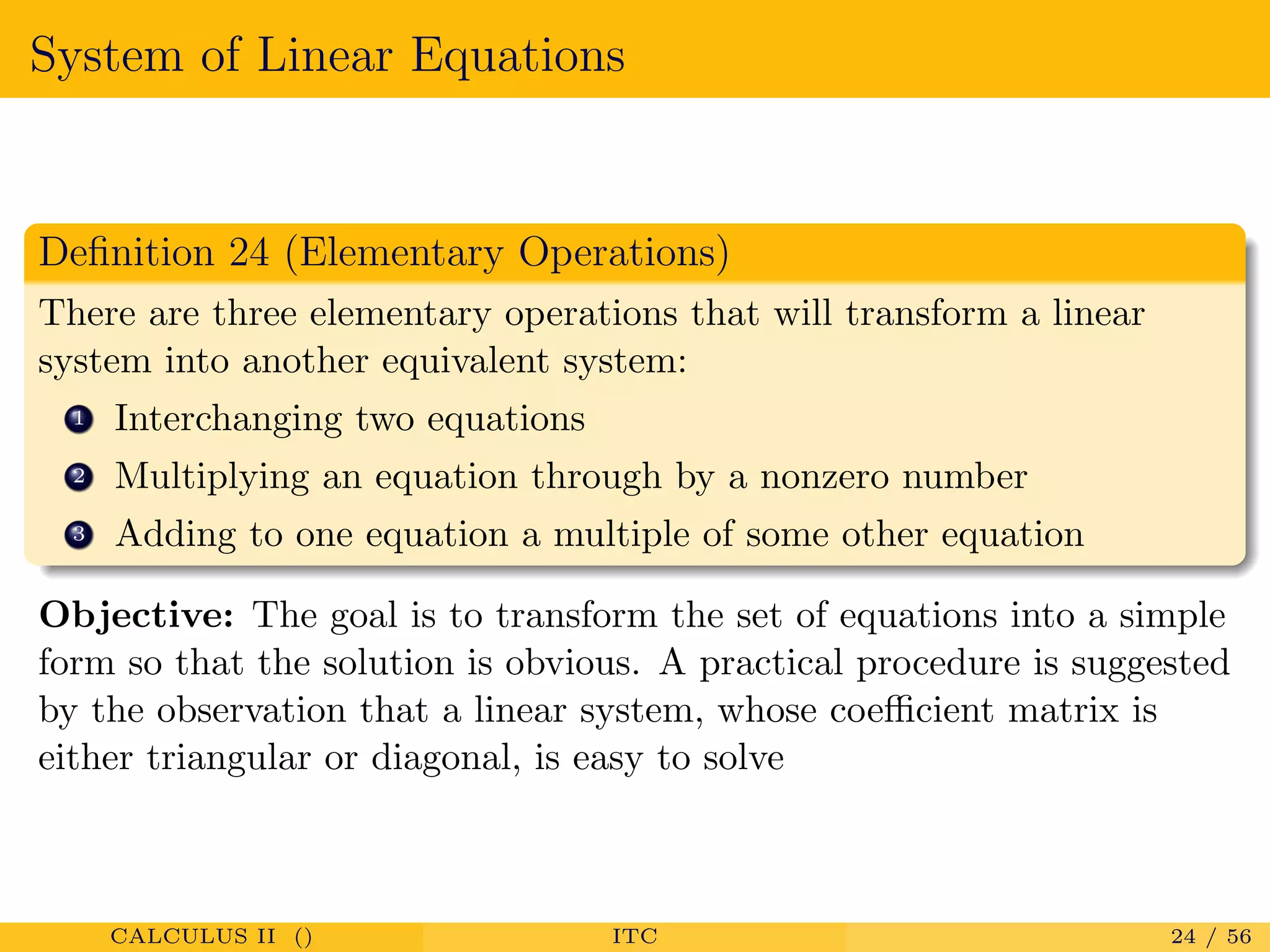
Description of elementary operations to transform linear systems and notation of augmented matrices.
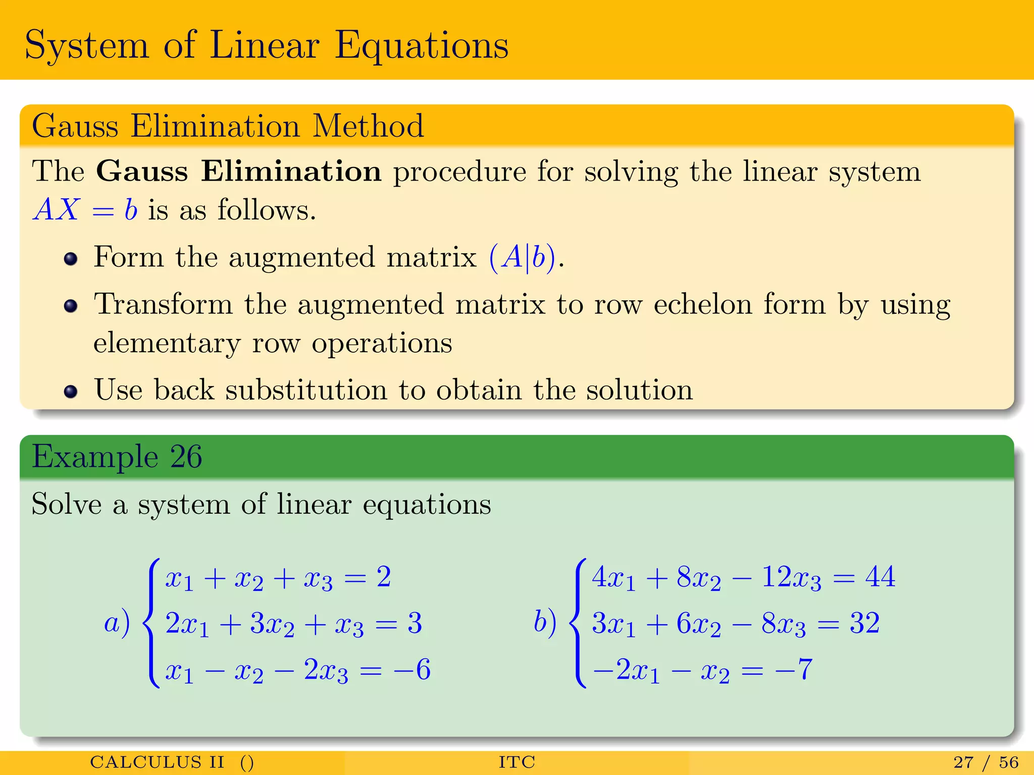
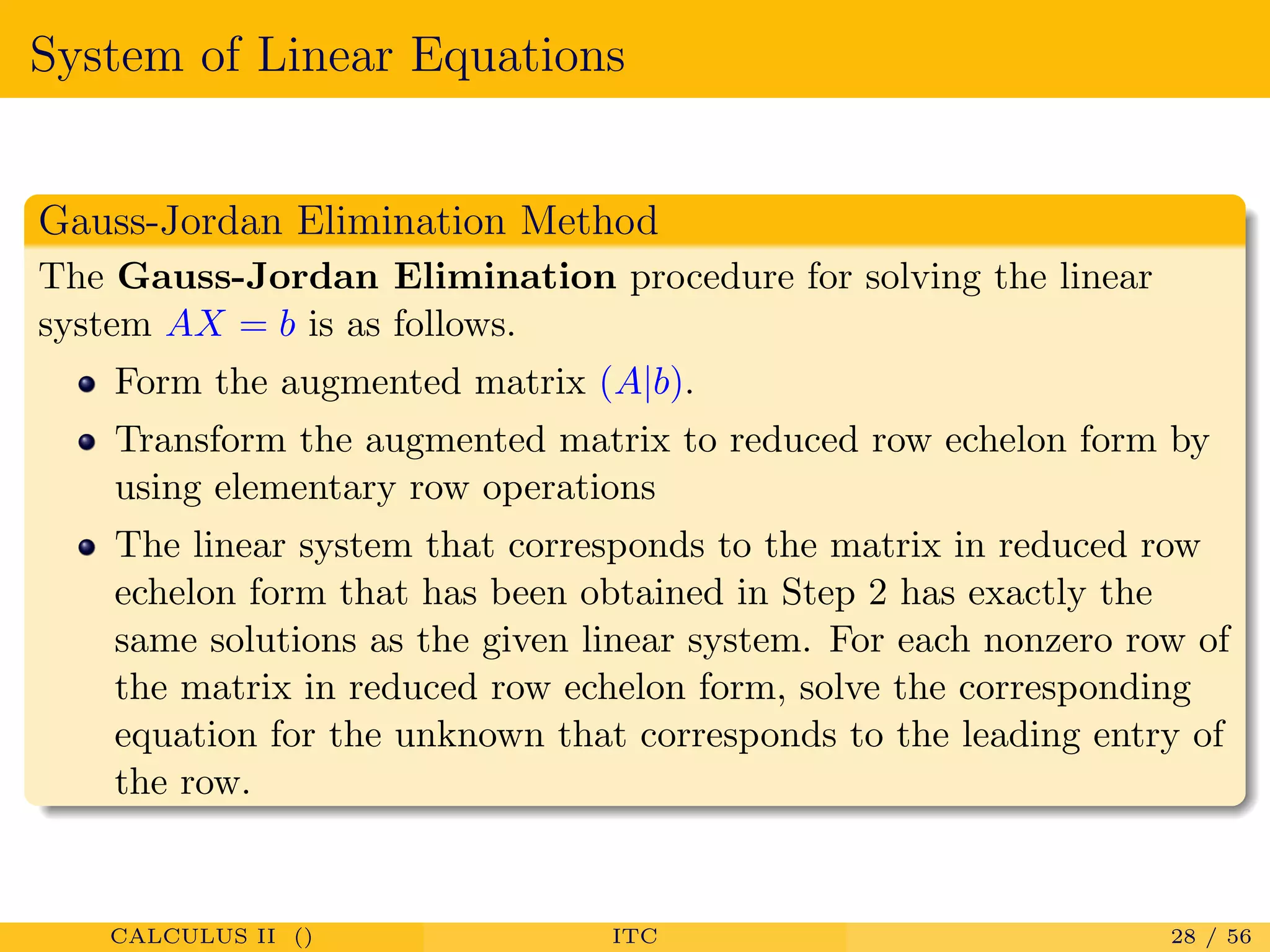
Gauss elimination and Gauss-Jordan elimination methods for solving linear systems.
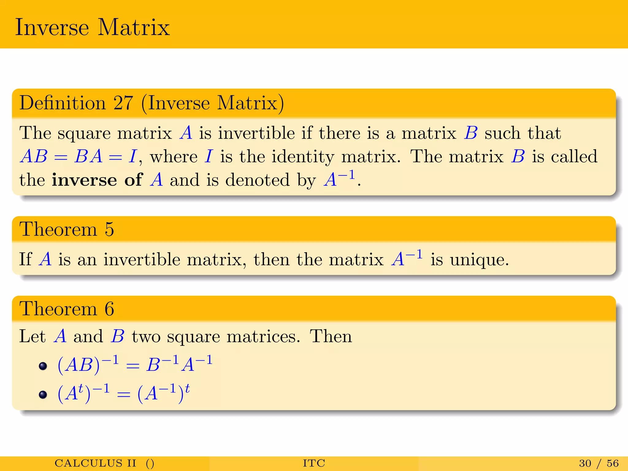
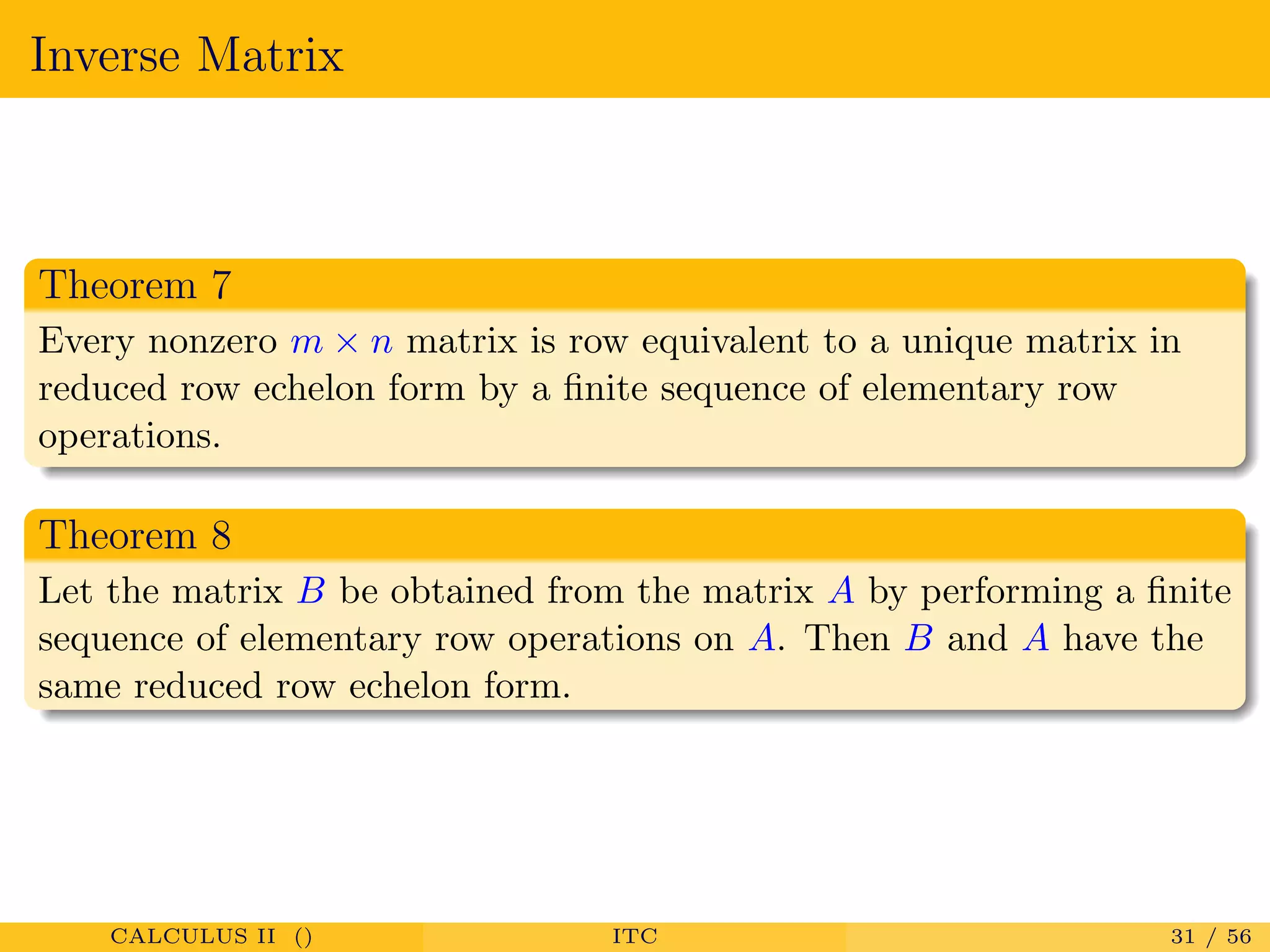
Definition and properties of inverse matrices, including uniqueness and relationships between matrices.
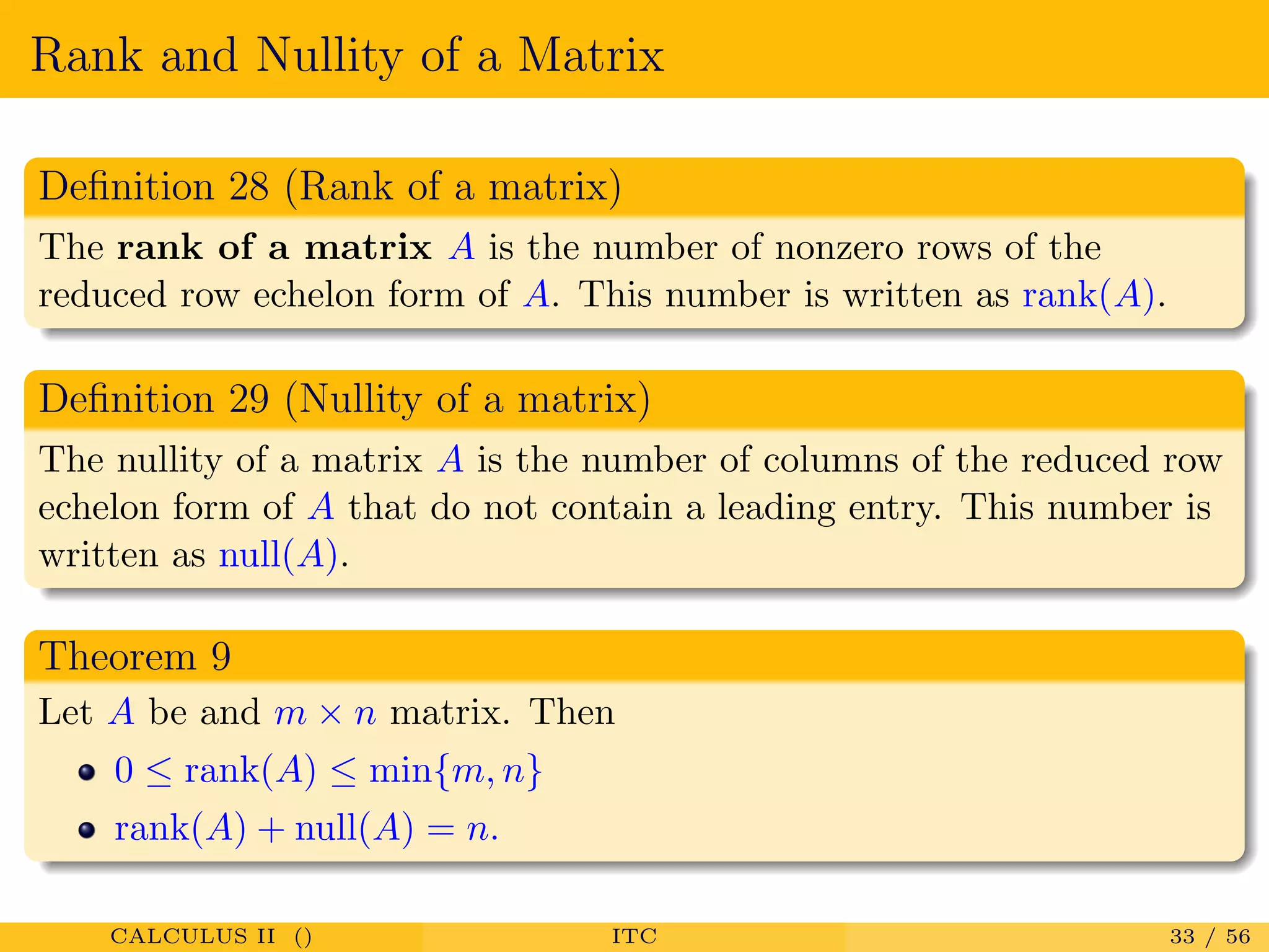
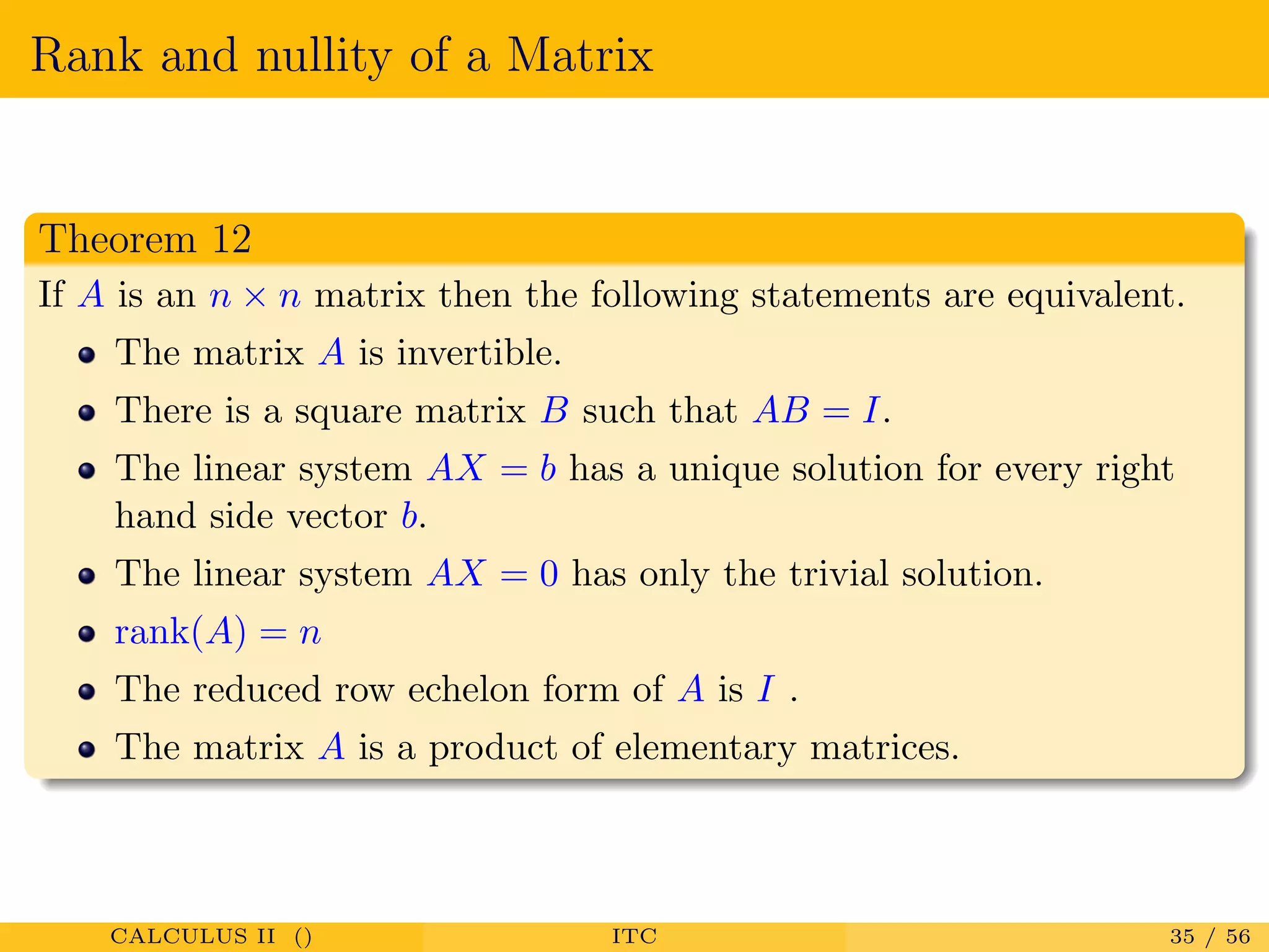
Definitions of rank and nullity of matrices, related theorems, and their implications.
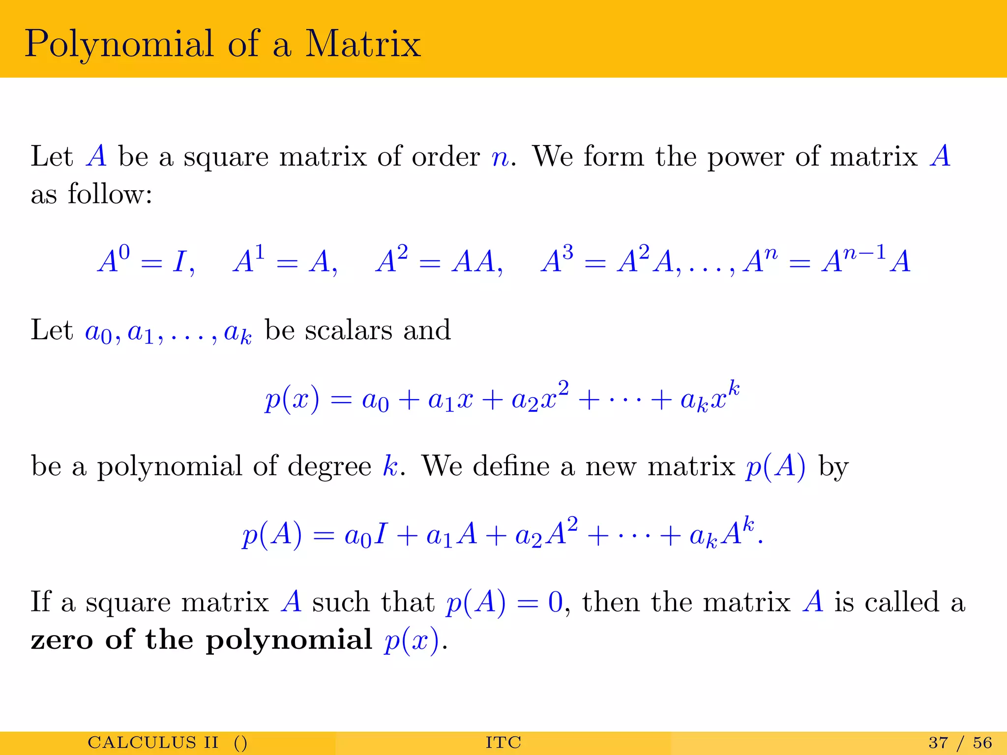
Definition of polynomials in the context of matrices, including forming new matrices with polynomials.
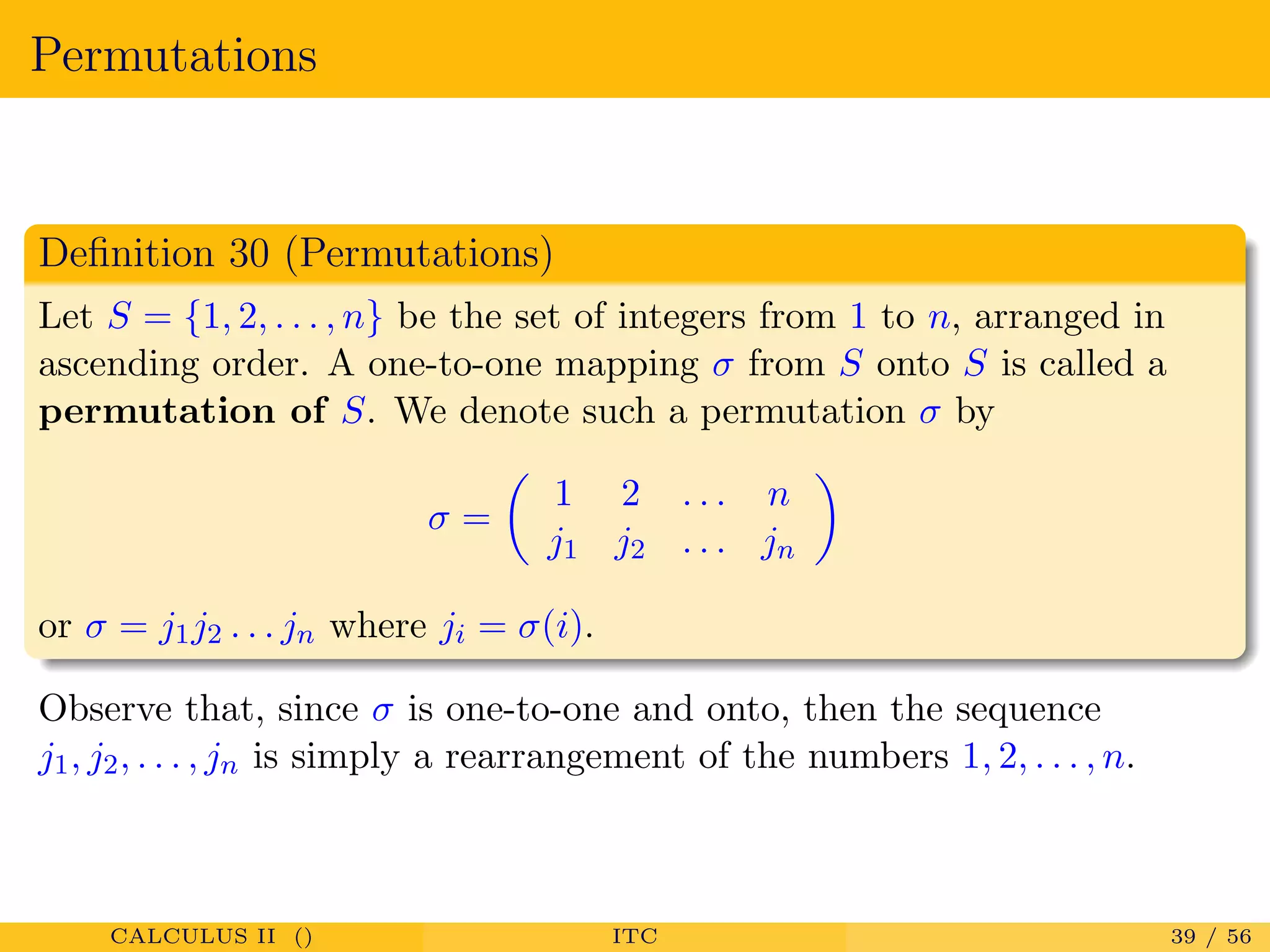
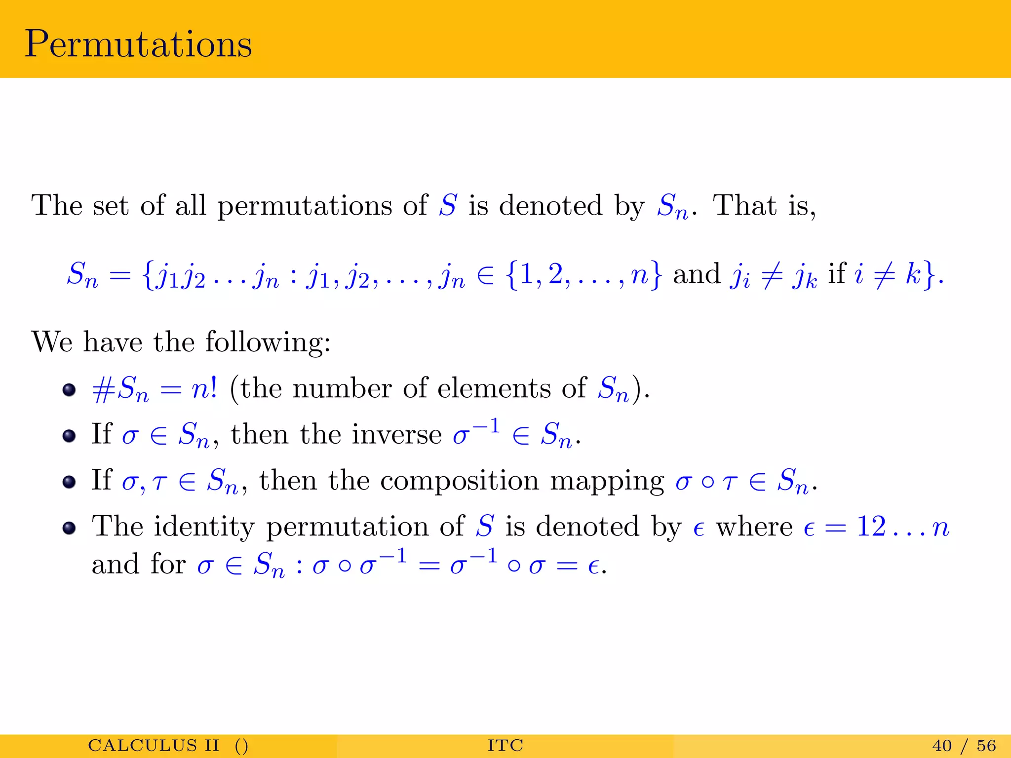
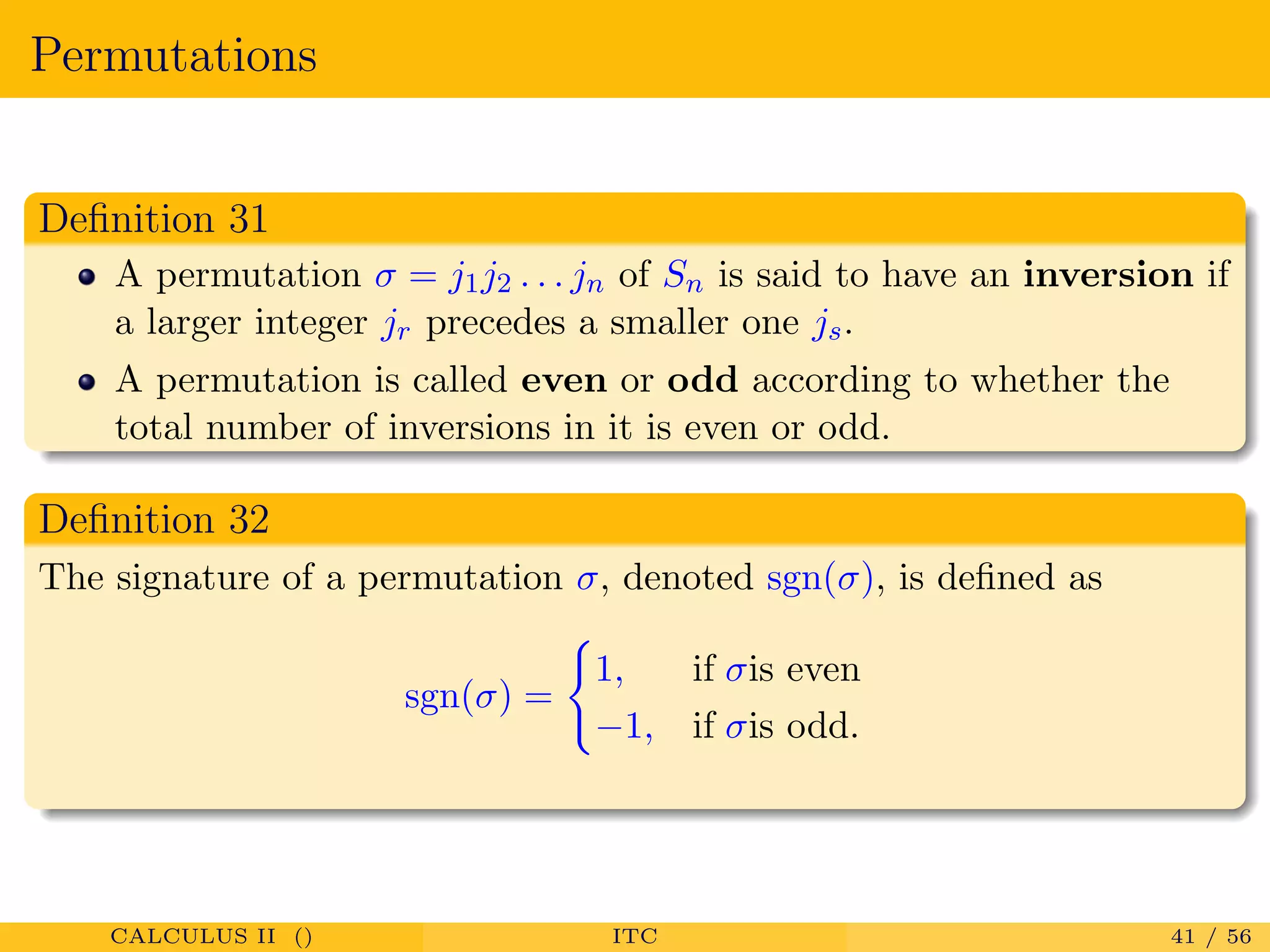
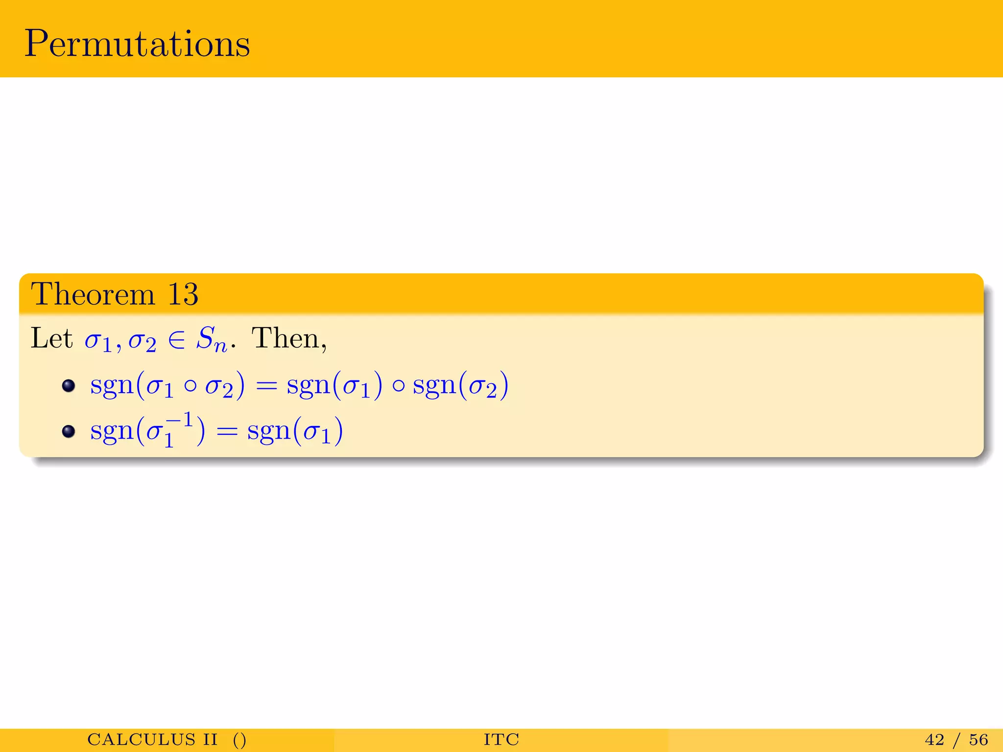
Introduction and definitions related to permutations, including the number of permutations and their characteristics.
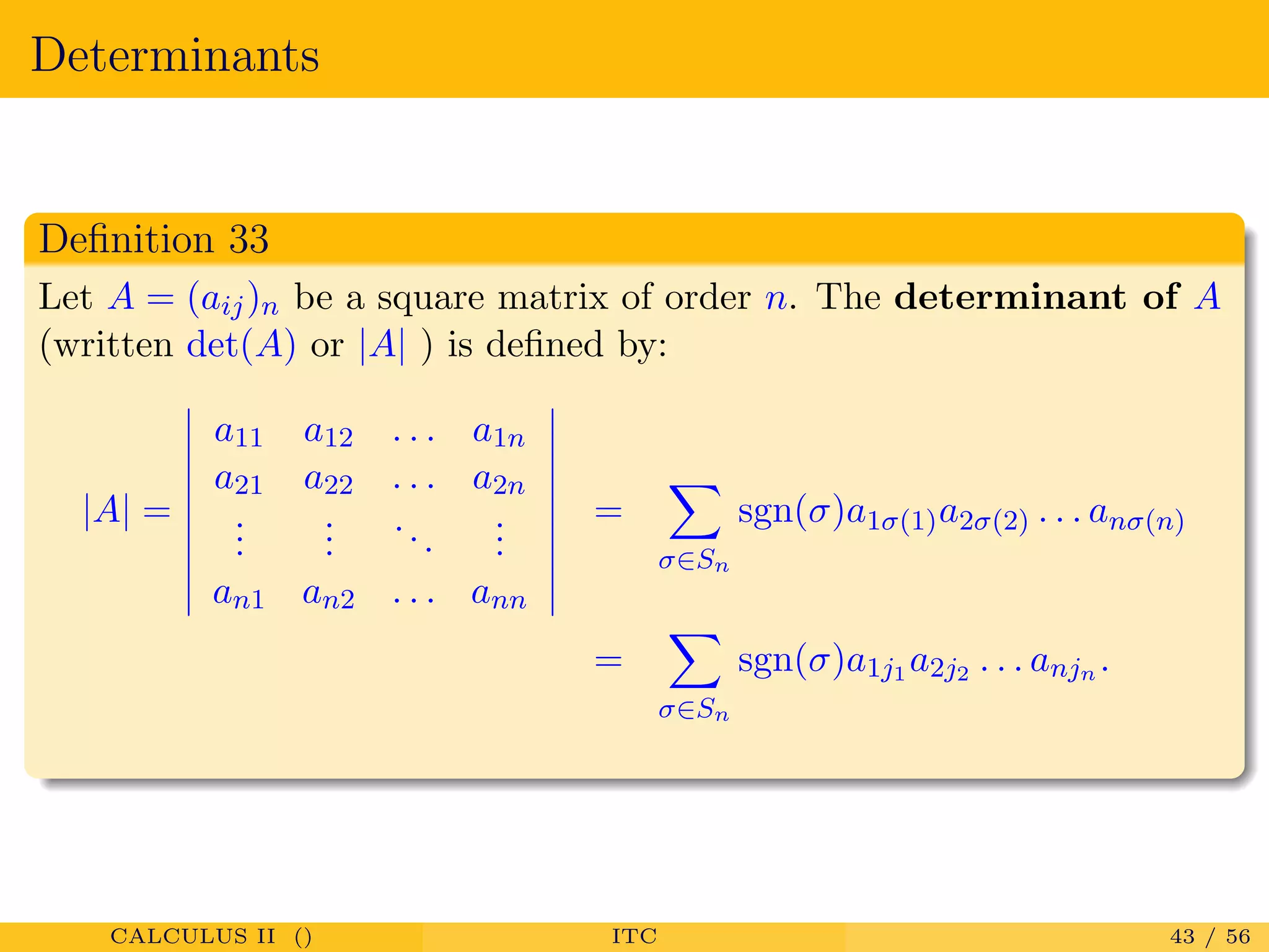
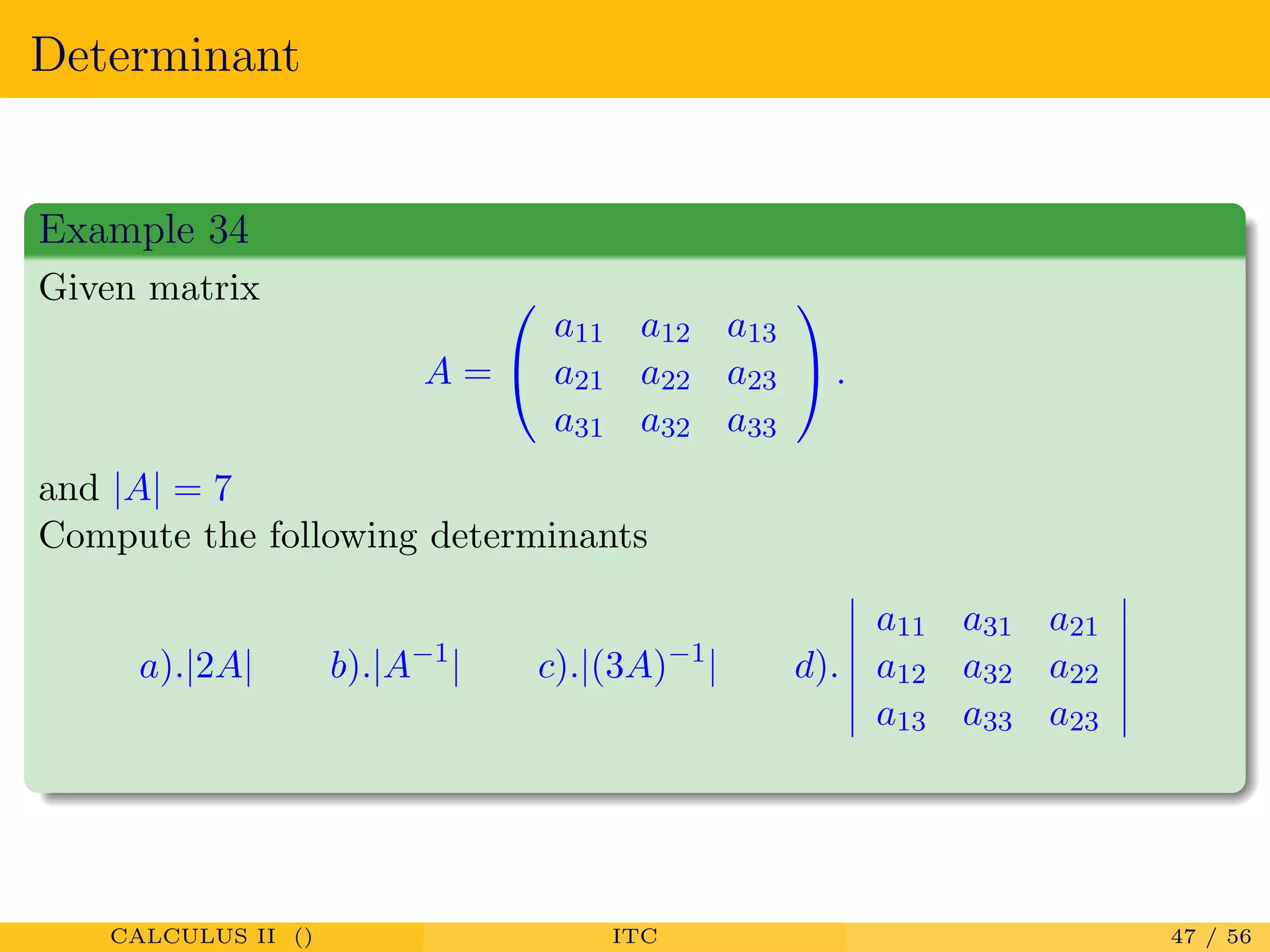
Definitions of determinants of square matrices and properties, as well as how they are calculated.
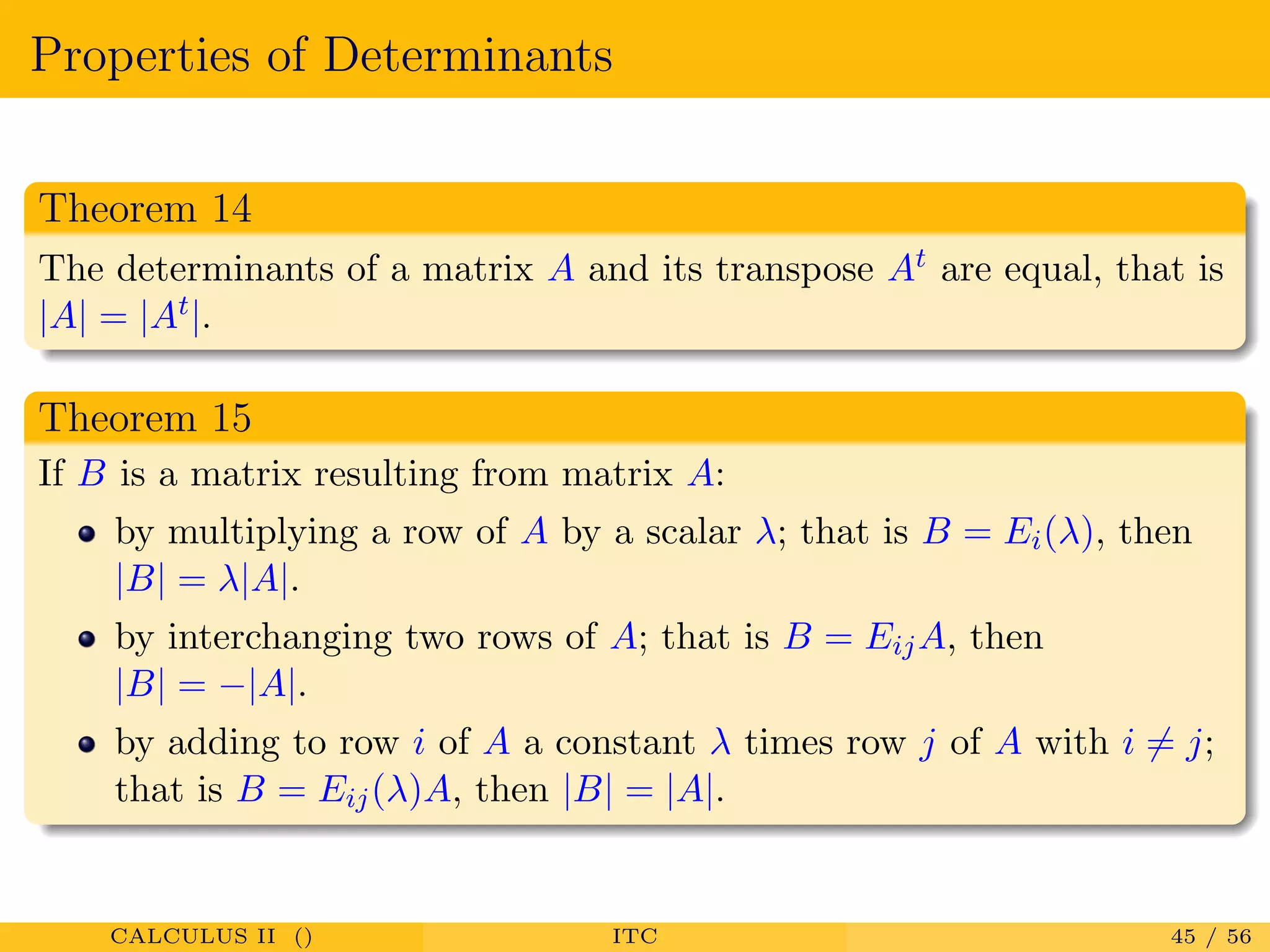
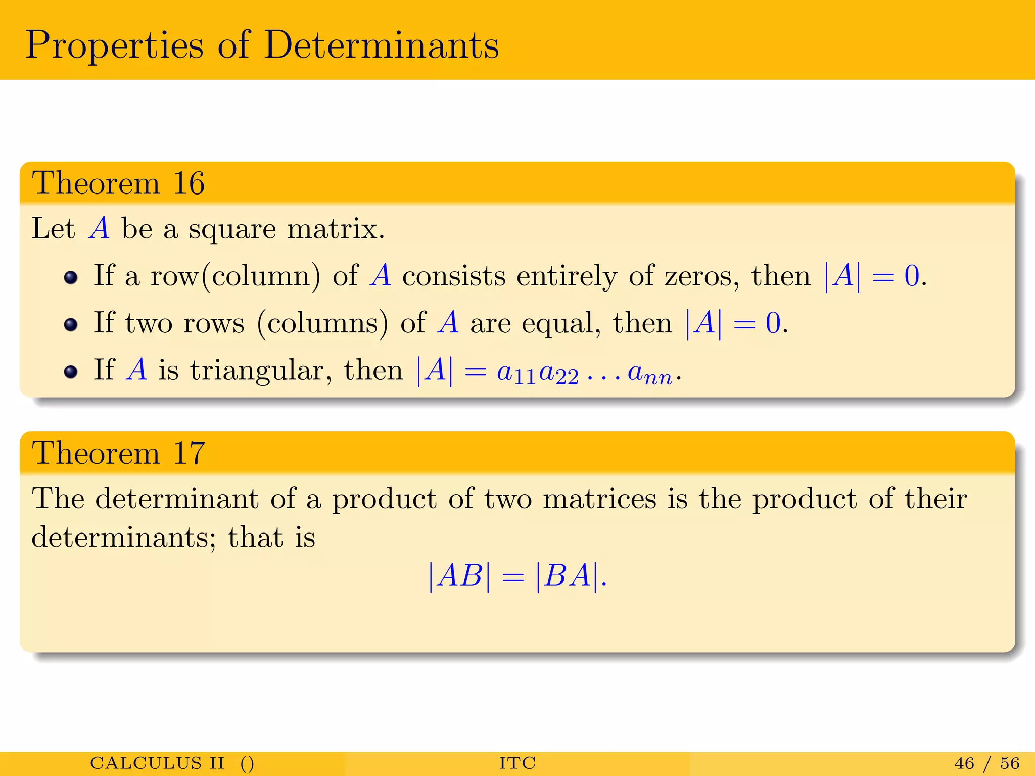
Theorems related to determinants including operations affecting determinants and their characteristics.
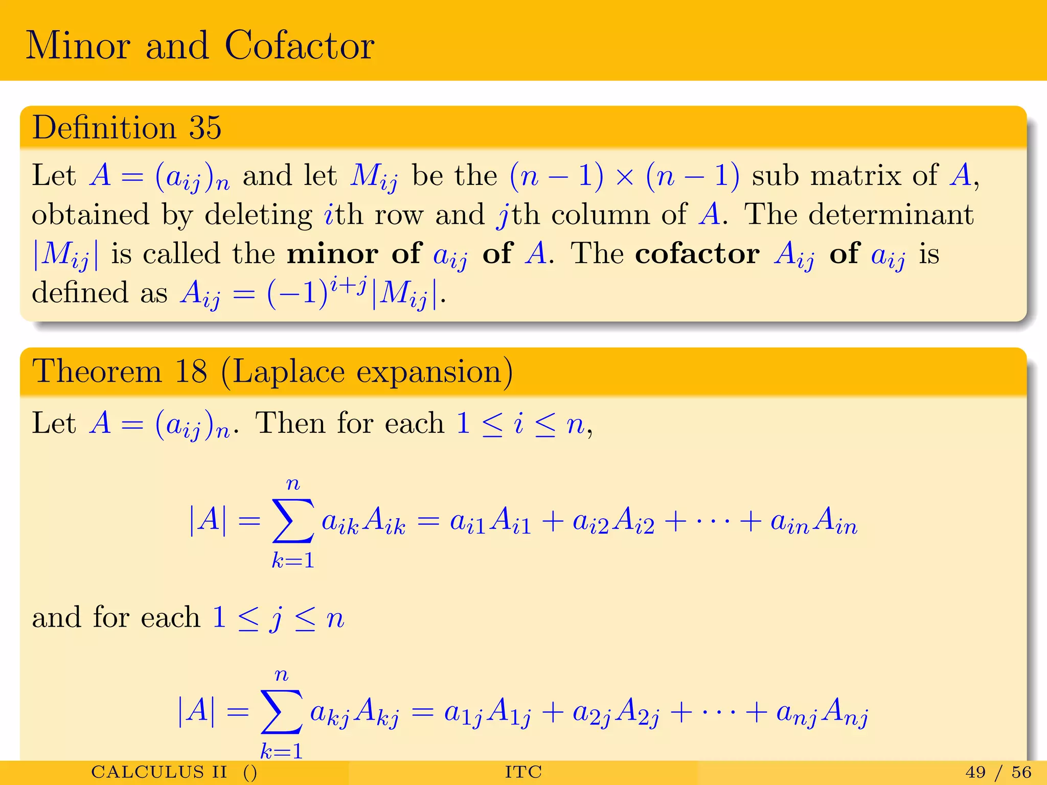
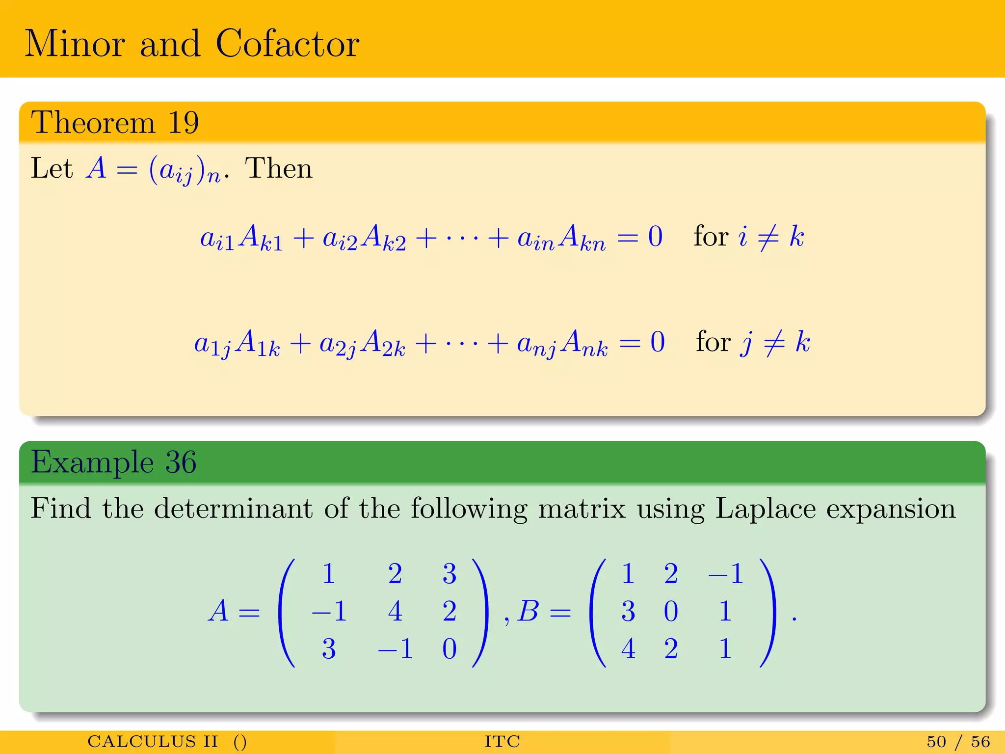
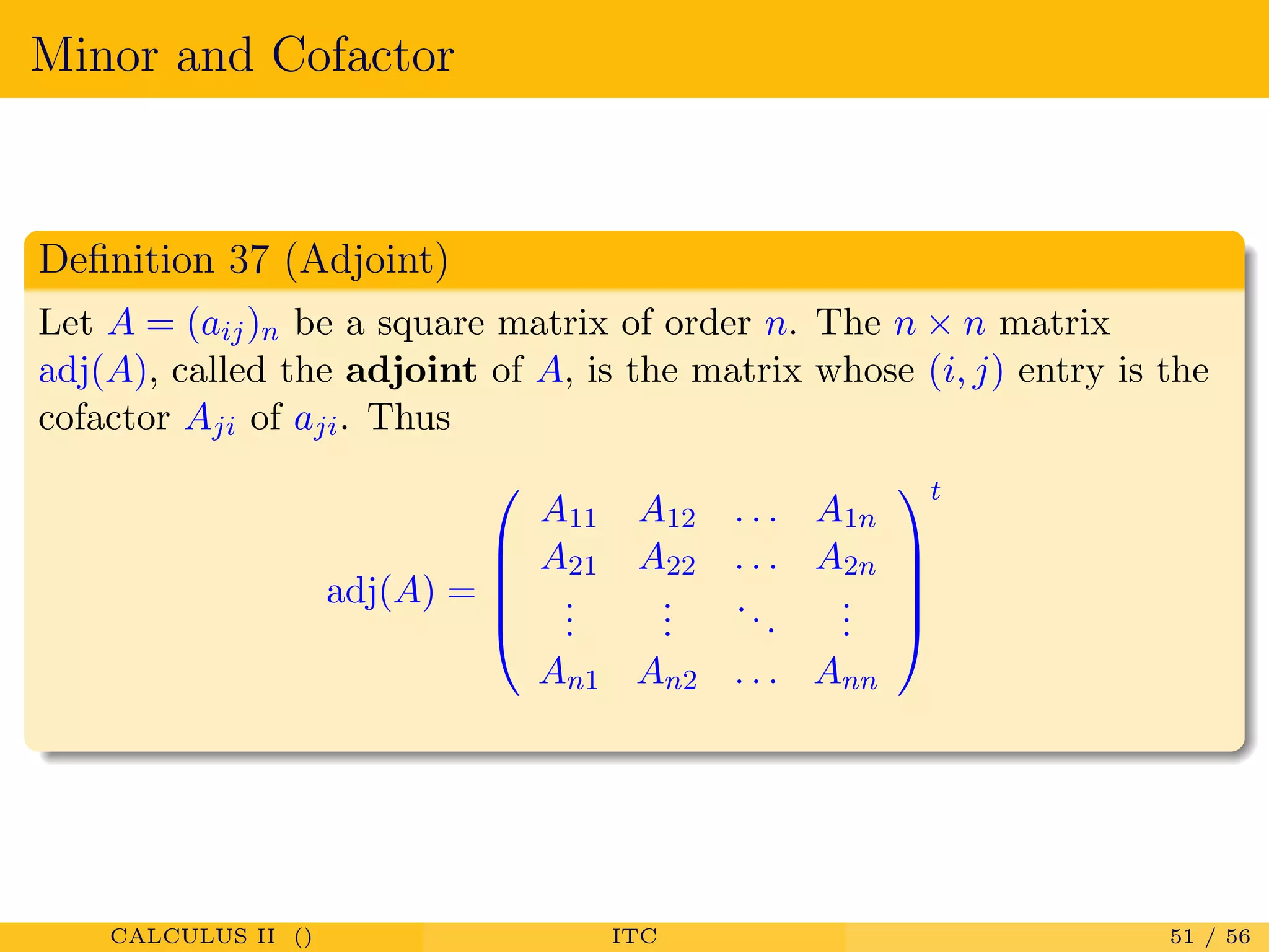
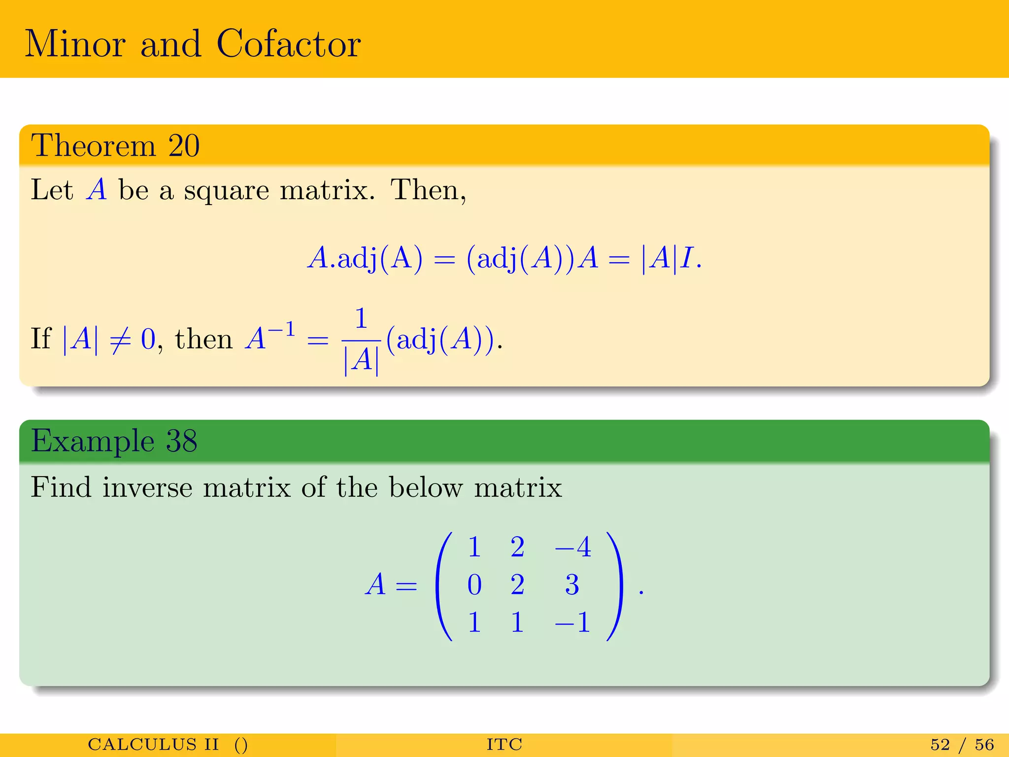
Definitions of minors and cofactors, including Laplace expansion for determining determinants.
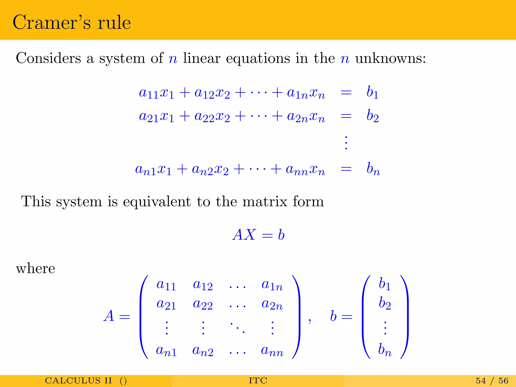
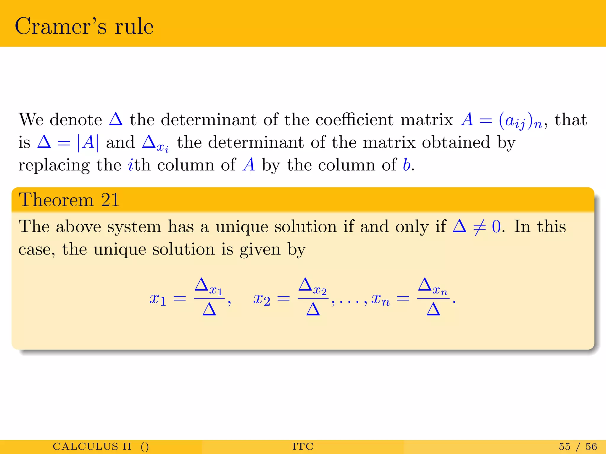
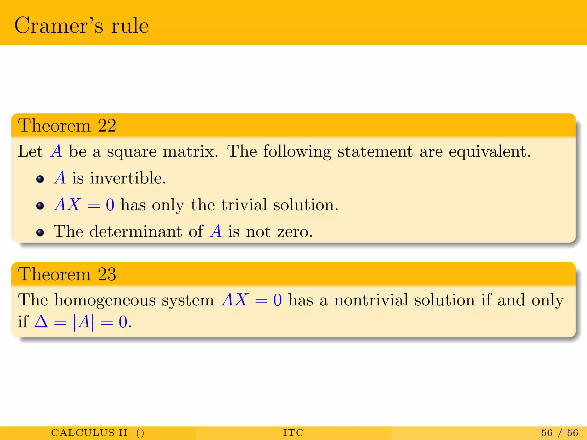
Definition and application of Cramer's rule for solving systems of linear equations using determinants.