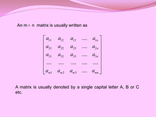
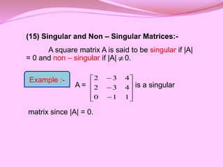
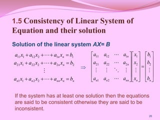
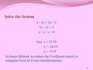
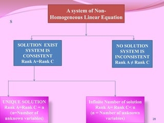
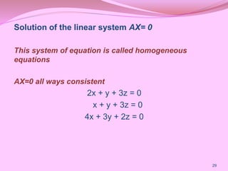
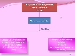
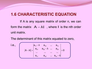
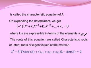
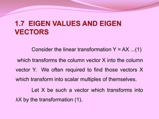
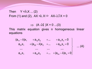
This document provides definitions and examples of different types of matrices including: real matrix, square matrix, row matrix, column matrix, null matrix, sub-matrix, diagonal matrix, scalar matrix, unit matrix, upper triangular matrix, lower triangular matrix, triangular matrix, single element matrix, equal matrices, singular and non-singular matrices. It also discusses elementary row and column transformations, rank of a matrix, solutions to homogeneous and non-homogeneous systems of linear equations, characteristic equations, eigenvectors and eigenvalues.

1. -227R1A1203
-Asrith chowdary
-IT(A)

2. MATRICES
CONTENT
1.1 INTRODUCTION
1.2 TYPES OF MATRICES
1.3 ELEMENTARY ROW AND COLUMN
TRANSFORMATION
1.4 RANK OF MATRIX
2

3. 3

4. 
MATRICES

5. An m n matrix is usually written as
A matrix is usually denoted by a single capital letter A, B or C
etc.
11 12 13 1
21 22 23 2
31 32 33 3
1 2 3
....
....
....
.... .... .... .... ....
....
n
n
n
m m m mn
a a a a
a a a a
a a a a
a a a a
 
 
 
 
 
 
 
 


6. Thus, an m n matrix A may be written as
A = , where i = 1, 2, 3, … , m ;
j = 1, 2, 3, … , n
In Algebra, the matrices have their largest
application in the theory of simultaneous
equations and linear transformations.

6
ij
a
 
 

7. 







7
2
0
1
3
5
1.2 TYPES OF MATRICES
(1) Real Matrix :- A matrix is said to be
real if all its elements are real numbers.
E.g., is a real matrix.

8. (2) Square Matrix:- A matrix in which the number
of rows is equal to the number of columns is called
a square matrix, otherwise, it is said to be
rectangular matrix.
i.e., a matrix A = is a square matrix if m = n
a rectangular matrix if m n
ij m n
a

 
 


9. A square matrix having n rows and n columns is
called “ n – rowed square matrix”,
is a 3 – rowed square matrix
The elements of a square matrix are
called its diagonal elements and the diagonal
along with these elements are called principal or
leading diagonal.
11 12 13
21 22 23
31 32 33
a a a
a a a
a a a
 
 
 
 
 
33
,
22
11 a
a
,
a

10. The sum of the diagonal elements of a
square matrix is called its trace or spur.
Thus, trace of the n rowed square matrix
A= is
ij
a
 
 







n
1
i
ij
nn
33
22
11 a
a
....
a
a
a

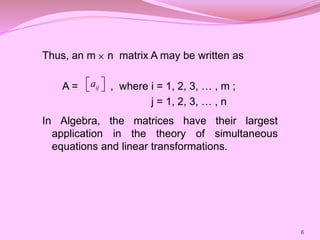
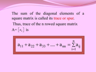
11. (3) Row Matrix :-
A matrix having only one row and any
number of columns,
i.e., a matrix of order 1 n is called a row
matrix.
[2 5 -3 0] is a row matrix.

Example:-

12. (4) Column Matrix:-
A matrix having only one column
and any number of rows,
i.e., a matrix of order m 1 is called a column
matrix.
is a column matrix.










1
0
2

Example:-

13. (5) Null Matrix:-
A matrix in which each element is zero
is called a null matrix or void matrix or zero matrix.
A null matrix of order m n is denoted by
=
13
 n
m
O 
Example :-






0
0
0
0
0
0
0
0
4
2
O 

14. (6) Sub - matrix :-
A matrix obtained from a given matrix A by
deleting some of its rows or columns or both is
called a sub – matrix of A.
is a sub – matrix of






4
1
0
3












2
4
6
1
7
0
5
3
5
2
1
0
Example:-

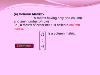
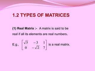
15. (7) Diagonal Matrix :-
A square matrix in which all non – diagonal
elements are zero is called a diagonal matrix.
i.e., A = [a ] is a diagonal matrix if a = 0 for i j.
is a diagonal matrix.
ij n
n ij 
Example:-











0
0
0
0
1
0
0
0
2

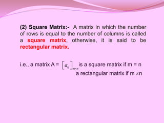
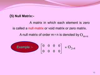
16. (8) Scalar Matrix:-
A diagonal matrix in which all the diagonal
elements are equal to a scalar, say k, is called a
scalar matrix.
i.e., A = [a ] is a scalar matrix if
is a scalar matrix.










2
0
0
0
2
0
0
0
2
ij n
n 





j
i
when
k
j
i
when
0
aij
Example :-

17. (9) Unit Matrix or Identity Matrix:-
A scalar matrix in which each diagonal
element is 1 is called a unit or identity matrix. It is
denoted by .
i.e., A = [a ] is a unit matrix if
is a unit matrix.
n
I
ij n
n 





j
i
when
1
j
i
when
0
aij
Example






1
0
0
1

18. (10) Upper Triangular Matrix.
A square matrix in which all the elements
below the principal diagonal are zero is called an
upper triangular matrix.
i.e., A = [a ] is an upper triangular matrix if a = 0
for i > j
is an upper triangular
matrix











3
0
0
5
1
0
4
3
2
ij n
n ij
Example:-

19. (11) Lower Triangular Matrix.
A square matrix in which all the elements
above the principal diagonal are zero is called a
lower triangular matrix.
i.e., A = [a ] is a lower triangular matrix if a = 0
for i < j
is a lower triangular
matrix.
ij n
n ij
Example:-










0
2
3
0
6
5
0
0
1

20. (12) Triangular Matrix:-
A triangular matrix is either upper
triangular or lower triangular.
(13) Single Element Matrix:-
A matrix having only one element is
called a single element matrix.
i.e., any matrix [3] is a single element matrix.

21. (14) Equal Matrices:-
Two matrices A and B are said to be equal iff
they have the same order and their corresponding
elements are equal.
i.e., if A = and B = , then A = B
iff a) m = p and n = q
b) a = b for all i and j.
q
p
ij]
b
[ 
n
m
ij]
a
[ 
ij ij

22. (15) Singular and Non – Singular Matrices:-
A square matrix A is said to be singular if |A|
= 0 and non – singular if |A| 0.
A = is a singular
matrix since |A| = 0.













1
1
0
4
3
2
4
3
2

Example :-

23. 1.3 ELEMENTARY ROW AND COLUMN
TRANSFORMATION
Some operations on matrices called as elementary
transformations. There are six types of elementary
transformations, three of then are row transformations and
other three of them are column transformations. There are
as follows
1) Interchange of any two rows or columns.
2) Multiplication of the elements of any row (or column)
by a non zero number k.
3) Multiplication to elements of any row or column by a
scalar k and addition of it to the corresponding elements
of any other row or column.
23

24. 1.4 RANK OF MATRIX
A positive integer ‘r’ is said to be the rank of a non- zero
matrix A if
1) There exists at least one non-zero minor of order r of A
and whose determinate is not equal to zero.
2) Every minor of order greater than r of A is zero.
The rank of a matrix A is denoted by ρ(A) .
24

25. 25

26. 1.5 Consistency of Linear System of
Equation and their solution
Solution of the linear system AX= B
26
n
n
nn
n
n
n
n
n
n
b
x
a
x
a
x
a
b
x
a
x
a
x
a
b
x
a
x
a
x
a
















2
2
1
1
2
2
2
22
1
21
1
1
2
12
1
11





































n
n
nn
n
n
n
n
b
b
b
x
x
x
a
a
a
a
a
a
a
a
a









2
1
2
1
2
1
2
22
21
1
12
11

If the system has at least one solution then the equations
are said to be consistent otherwise they are said to be
inconsistent.

27. Solve the System
x - 2y + 3z = 2
2x - 3z = 3
x + y +z = 0
Ans x = 21/19
y = -16/19
z = -5/19
In Gauss Method, we reduce the Coefficient matrix to
triangular form by E-row transformations.
27

28. s
28
A system of Non-
Homogeneous Linear Equation
SOLUTION EXIST
SYSTEM IS
CONSISTENT
Rank A=Rank C
NO SOLUTION
SYSTEM IS
INCONSISTENT
Rank A ≠ Rank C
UNIQUE SOLUTION
Rank A=Rank C = n
(n=Number of
unknown variables)
Infinite Number of solution
Rank A= Rank C< n
(n = Number of unknown
variables)

29. Solution of the linear system AX= 0
This system of equation is called homogeneous
equations
AX=0 all ways consistent
2x + y + 3z = 0
x + y + 3z = 0
4x + 3y + 2z = 0
29

30. s
30
A system of Homogeneous
Linear Equation
AX=0
Always has a solution
Unique Or Trivial Solution
Rank A = n (n=Number of
unknown variables)
(Each Unknown equal to
zero)
Infinite Or Non-Trivial
solution
Rank A< n
(n = Number of unknown
variables)
Find R(A)

31. Vectors :
Any ordered n-tuple of numbers is called n-vectors . By an
ordered n-tuple we means a set consisting of n-numbers in
which the place of each number is fixed . If x1, x2, x3, ….. xn
is called n-vector.
Eg. (1 ,2 ,3 ,4) is a 4 vectors
Linearly Dependent :
Vectors (Matrices ) x1, x2, x3, ….. xn are said to be dependent
.if there exist r scalars λ1, λ2, λ3, ….. λn . Not all zero . If the
relation of the type
31

32. λ1 x1+ λ2 x2+ λ3 x3+….. λn xn =0
λ1 ≠ λ2 ≠ λ3 =0
λ4 =λ5=….. λn =0
Linearly Independent :
Vectors (Matrices ) x1, x2, x3, ….. xn are said to be
independent .if there exist r scalars λ1, λ2, λ3, ….. λn . All
are zero . If the relation of the type
λ1 x1+ λ2 x2+ λ3 x3+….. λn xn =0
λ1 = λ2 = λ3 =….. λn = 0
32

33. Linearly dependence and independence of
vectors by Rank Method
1) Rank of MATRIX = Number of vector
(then vector are Linearly Independent)
2) Rank of MATRIX < Number of vector
(then vector are Linearly dependent)
t
33

34. 1.6 CHARACTERISTIC EQUATION
If A is any square matrix of order n, we can
form the matrix , where is the nth order
unit matrix.
The determinant of this matrix equated to zero,
i.e.,
I
λ
A  I
0
λ
a
...
a
a
...
...
...
...
a
...
λ
a
a
a
...
a
λ
a
λ
A
nn
n2
n1
2n
22
21
1n
12
11





 I

35. 0
k
...
λ
k
λ
k
λ
1)
( n
2
n
2
1
n
1
n
n





 

ij

36. Consider the linear transformation Y = AX ...(1)
which transforms the column vector X into the column
vector Y. We often required to find those vectors X
which transform into scalar multiples of themselves.
Let X be such a vector which transforms into
λX by the transformation (1).
1.7 EIGEN VALUES AND EIGEN
VECTORS

37. Then Y = X ... (2)
From (1) and (2), AX = X AX- X = 0
(A - )X = 0 ...(3)
This matrix equation gives n homogeneous linear
equations
... (4)
I


 























0
λ)x
(a
...
x
a
x
a
....
....
....
....
0
x
a
...
λ)x
(a
x
a
0
x
a
...
x
a
λ)x
(a
n
nn
2
n2
1
n1
n
2n
2
22
1
21
n
1n
2
12
1
11
 I

38. These equations will have a non-trivial solution only
if the co-efficient matrix A - is singular
i.e., if |A - | = 0 ... (5)
Corresponding to each root of (5), the
homogeneous system (3) has a non-zero solution
X = is called an eigen vector or latent
vector

I
I













4
2
1
x
...
x
x

39. Properties of Eigen Values:-
1.The sum of the eigen values of a matrix is the sum
of the elements of the principal diagonal.
2.The product of the eigen values of a matrix A is
equal to its determinant.
3.If is an eigen value of a matrix A, then 1/ is
the eigen value of A-1 .
4.If is an eigen value of an orthogonal matrix, then
1/ is also its eigen value.
39
 



40. PROPERTY 1:- If λ1, λ2,…, λn are the eigen values of
A, then
i. k λ1, k λ2,…,k λn are the eigen values of the matrix
kA, where k is a non – zero scalar.
ii. are the eigen values of the inverse
matrix A-1.
iii. are the eigen values of Ap, where p
is any positive integer.
n
2
1 λ
1
,...,
λ
1
,
λ
1
p
n
p
2
p
1 λ
...,
,
λ
,
λ
40

41. 7. Find the eigen values and eigen vectors of the
matrix A =
Solution:- The characteristic equation of the given
matrix is















0
2
1
6
1
2
3
2
2
0
|
I
A
| 


0
2
1
6
1
2
3
2
2













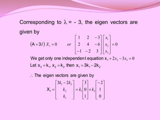
42. Thus,
5
3,
3,
λ
0
5)
3)(λ
3)(λ
(λ
0
15)
2λ
3)(λ
(λ
it.
satisfies
3
λ
trial,
By
0
45
21λ
λ
λ
0
λ)]
1(1
4
3[
6]
2λ
2[
12]
λ)
λ(1
λ)[
2
(
2
2
3



































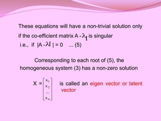
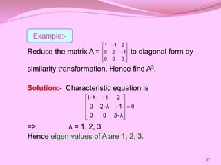
the eigen values of A are -3, -3, 5.

43. Corresponding to = - 3, the eigen vectors are
given by

 































 




































0
1
2
1
0
3
2
3
0
3
2
0
3
2
1
6
4
2
3
2
1
0
2
1
1
2
2
1
3
2
3
2
1
1
k
k
k
k
k
k
x
x
x
x
x
or
X
I
1
2
1
1
2
2
1
3
1
X
by
given
are
vectors
eigen
The
2k
3k
x
then
k
x
,
k
x
Let
x
equation
t
independen
one
only
get
We
3
A

44. Corresponding to λ = 5, the eigen vectors are
given by (A – 5 I )X2 = 0.
0
5
2
0
3
2
0
3
2
7
0
0
0
5
2
1
6
4
2
3
2
7
3
2
1
3
2
1
3
2
1
3
2
1



















































x
x
x
x
x
x
x
x
x
x
x
x

45. 


























1
2
1
k
X
k
x
2k
x
,
k
x
(say)
k
1
x
2
x
1
x
2
2
x
5
3
x
6
-
10
x
3
2
3
3
3,
2
3
1
3
3
2
1
3
2
1
by
given
are
vectors
eigen
the
Hence
,
equations.
two
first
From
45

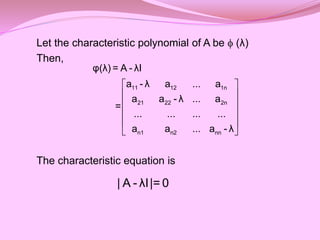
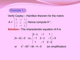
46. 1.8 CAYLEY HAMILTON THEOREM
Every square matrix satisfies its own
characteristic equation.
Let A = [aij]n×n be a square matrix
then,
n
n
nn
2
n
1
n
n
2
22
21
n
1
12
11
a
...
a
a
....
....
....
....
a
...
a
a
a
...
a
a
A















47. Let the characteristic polynomial of A be  (λ)
Then,
The characteristic equation is
 
 
 
 
 
 
11 12 1n
21 22 2n
n1 n2 nn
φ(λ) = A - λI
a - λ a ... a
a a - λ ... a
=
... ... ... ...
a a ... a - λ
| A - λI|= 0

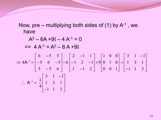
48. Note 1:- Premultiplying equation (1) by A-1 , we
have
 n n-1 n-2
0 1 2 n
n n-1 n-2
0 1 2 n
We are to prove that
p λ +p λ +p λ +...+p = 0
p A +p A +p A +...+p I= 0 ...(1)
I

n-1 n-2 n-3 -1
0 1 2 n-1 n
-1 n-1 n-2 n-3
0 1 2 n-1
n
0 =p A +p A +p A +...+p +p A
1
A =- [p A +p A +p A +...+p I]
p

49. This result gives the inverse of A in terms of
(n-1) powers of A and is considered as a practical
method for the computation of the inverse of the
large matrices.
Note 2:- If m is a positive integer such that m > n
then any positive integral power Am of A is linearly
expressible in terms of those of lower degree.

50. Verify Cayley – Hamilton theorem for the matrix
A = . Hence compute A-1 .
Solution:- The characteristic equation of A is














2
1
1
1
2
1
1
1
2
tion)
simplifica
(on
0
4
9λ
6λ
λ
or
0
λ
2
1
1
1
λ
2
1
1
1
λ
2
i.e.,
0
λI
A
2
3














Example 1:-

51. To verify Cayley – Hamilton theorem, we have to
show that A3 – 6A2 +9A – 4I = 0 … (1)
Now,


























































































22
21
21
21
22
21
21
21
22
2
1
1
1
2
1
1
1
2
6
5
5
5
6
5
5
5
6
6
5
5
5
6
5
5
5
6
2
1
1
1
2
1
1
1
2
2
1
1
1
2
1
1
1
2
2
3
2
A
A
A
A

52. A3 -6A2 +9A – 4I = 0
= - 6 + 9
-4
=
This verifies Cayley – Hamilton theorem.















22
21
21
21
22
21
21
21
22














6
5
5
5
6
5
5
5
6














2
1
1
1
2
1
1
1
2










1
0
0
0
1
0
0
0
1
0
0
0
0
0
0
0
0
0
0












53. Now, pre – multiplying both sides of (1) by A-1 , we
have
A2 – 6A +9I – 4 A-1 = 0
=> 4 A-1 = A2 – 6 A +9I







































































3
1
1
1
3
1
1
1
3
4
1
3
1
1
1
3
1
1
1
3
1
0
0
0
1
0
0
0
1
9
2
1
1
1
2
1
1
1
2
6
6
5
5
5
6
5
5
5
6
4
1
1
A
A
53

54. 1.9 DIAGONALISATION OF A
MATRIX
Diagonalisation of a matrix A is the
process of reduction A to a diagonal form.
If A is related to D by a similarity transformation,
such that D = M-1AM then A is reduced to the
diagonal matrix D through modal matrix M. D is
also called spectral matrix of A.
54

55. REDUCTION OF A MATRIX TO
DIAGONAL FORM
If a square matrix A of order n has n linearly
independent eigen vectors then a matrix B can
be found such that B-1AB is a diagonal matrix.
Note:- The matrix B which diagonalises A is called
the modal matrix of A and is obtained by
grouping the eigen vectors of A into a square
matrix.
55

56. Similarity of matrices:-
A square matrix B of order n is said to be a
similar to a square matrix A of order n if
B = M-1AM for some non singular
matrix M.
This transformation of a matrix A by a non –
singular matrix M to B is called a similarity
transformation.
Note:- If the matrix B is similar to matrix A, then B
has the same eigen values as A.
56

57. Reduce the matrix A = to diagonal form by
similarity transformation. Hence find A3.
Solution:- Characteristic equation is
=> λ = 1, 2, 3
Hence eigen values of A are 1, 2, 3.












3
0
0
1
2
0
2
1
1
57
0













λ
-
3
0
0
1
λ
-
2
0
2
1
λ
1-
Example:-

58. Corresponding to λ = 1, let X1 = be the eigen
vector then










3
2
1
x
x
x


























































0
0
1
k
X
x
0
x
,
k
x
0
2x
0
x
x
0
2x
x
0
0
0
x
x
x
2
0
0
1
1
0
2
1
0
0
X
)
I
(A
1
1
3
2
1
1
3
3
2
3
2
3
2
1
1
58

59. Corresponding to λ = 2, let X2 = be the eigen
vector then,










3
2
1
x
x
x



























































0
1
-
1
k
X
x
-k
x
,
k
x
0
x
0
x
0
2x
x
x
0
0
0
x
x
x
1
0
0
1
0
0
2
1
1
-
0
X
)
(A
2
2
3
2
2
2
1
3
3
3
2
1
3
2
1
2
0
,
I
2
59

60. Corresponding to λ = 3, let X3 = be the eigen
vector then,










3
2
1
x
x
x




























































2
2
-
3
k
X
x
k
-
x
,
k
x
0
x
0
2x
x
x
0
0
0
x
x
x
0
0
0
1
1
-
0
2
1
2
-
0
X
)
(A
3
3
1
3
3
3
2
3
3
2
1
3
2
1
3
3
2
2
3
,
2
I
3
k
x
60

61. Hence modal matrix is



























 
















2
1
0
0
1
1
-
0
2
1
-
1
1
M
M
Adj.
M
1
-
0
0
2
2
0
1
2
2
-
M
Adj.
2
M
2
0
0
2
1
-
0
3
1
1
M
1
61

62. 



















































3
0
0
0
2
0
0
0
1
2
0
0
2
1
-
0
3
1
1
3
0
0
1
2
0
2
1
1
2
1
0
0
1
1
-
0
2
1
1
1
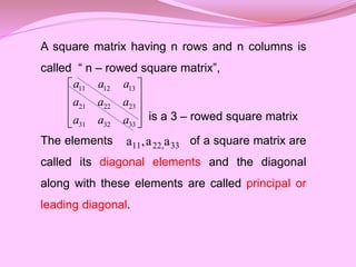
AM
M 1
62
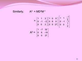
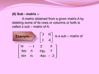
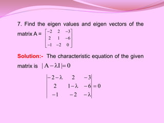
Now, since D = M-1AM
=> A = MDM-1
A2 = (MDM-1) (MDM-1)
= MD2M-1 [since M-1M = I]

63. Similarly, A3 = MD3M-1
=
A3 =















































27
0
0
19
-
8
0
32
7
-
1
2
1
0
0
1
1
-
0
2
1
1
1
27
0
0
0
8
0
0
0
1
2
0
0
2
1
-
0
3
1
1
63

64. Orthogonal Transformation
 Let A be a Symmetric Matrix, then
 AA ʹ = I
 We know that ,diagonalisation transformation of a
Symmetric Matrix is D = M-1AM
 If we Normalize each Eigen vector and use then
to form the Normalized Model Matrix N
 Then N is an Orthogonal Matrix
 D = NʹAN
 Transforming A into D by means of transformation
D = NʹAN is called Orthogonal transformation. 64
I
I
I
I

65. THANK YOU