Downloaded 10 times
![Example 1: General Solution (9 of 12)
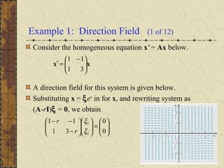
The two solutions of x' = Ax are
The Wronskian of these two solutions is
Thus x(1)
and x(2)
are fundamental solutions, and the general
solution of x' = Ax is
[ ] 0)(, 4
222
22
)2()1(
≠−=
−−
= t
ttt
tt
e
etee
tee
tW xx
−
+
−
+
−
=
+=
ttt
etecec
tctct
22
2
2
1
)2(
2
)1(
1
1
0
1
1
1
1
)()()( xxx
ttt
etetet 22)2(2)1(
1
0
1
1
)(,
1
1
)(
−
+
−
=
−
= xx](https://image.slidesharecdn.com/ch078-150731094838-lva1-app6891/85/Ch07-8-10-320.jpg)
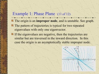
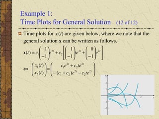
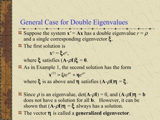
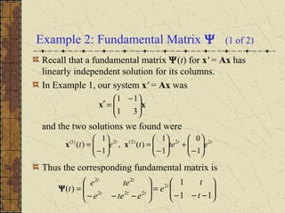
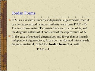

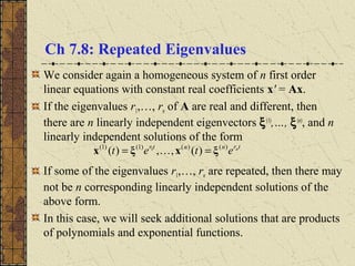
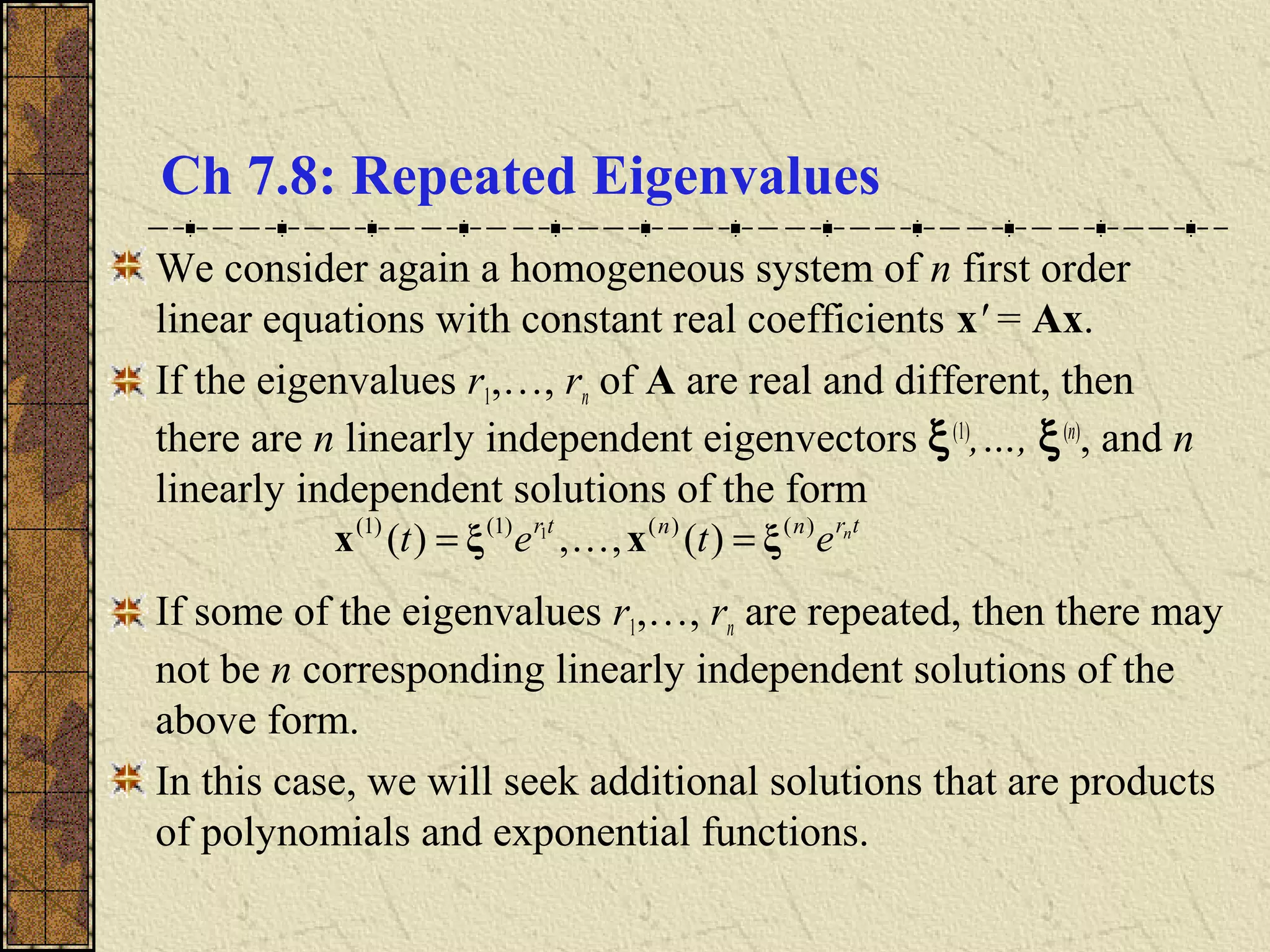
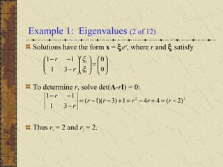
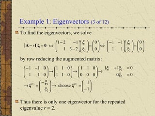
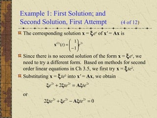
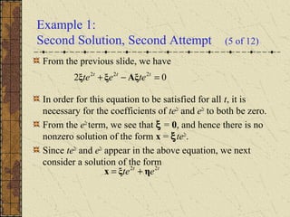
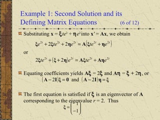
The document discusses repeated eigenvalues in systems of linear differential equations. If some eigenvalues are repeated, there may not be n linearly independent solutions of the form x = ξert. Additional solutions must be sought that are products of polynomials and exponential functions. For a double eigenvalue r, the first solution is x(1) = ξert, where ξ satisfies (A-rI)ξ = 0. The second solution has the form x(2) = ξtert + ηert, where η satisfies (A-rI)η = ξ and η is called a generalized eigenvector.