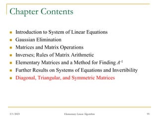
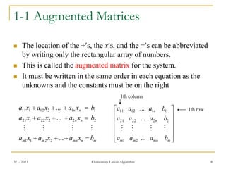
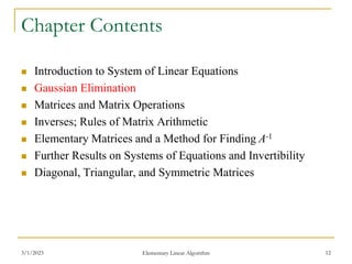
The chapter covers systems of linear equations and matrices. It introduces linear equations and systems of linear equations. It describes using elementary row operations to solve systems, representing systems as augmented matrices, and reducing matrices to row echelon and reduced row echelon form through row operations. It also covers diagonal, triangular, and symmetric matrices.
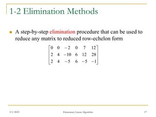
![3/1/2023 Elementary Linear Algorithm 31
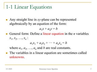
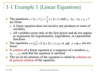
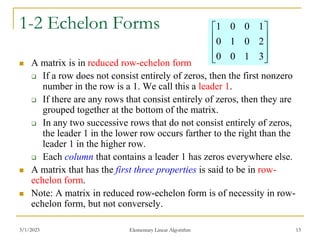
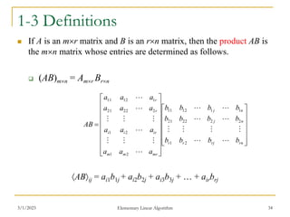
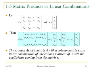
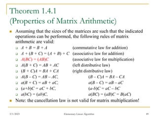
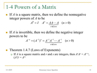
1-3 Definition and Notation
A matrix is a rectangular array of numbers. The numbers
in the array are called the entries in the matrix
A general mn matrix A is denoted as
The entry that occurs in row i and column j of matrix A
will be denoted aij or Aij. If aij is real number, it is
common to be referred as scalars
The preceding matrix can be written as [aij]mn or [aij]
mn
m
m
n
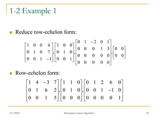
n
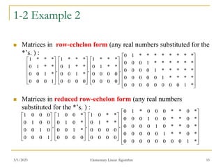
a
a
a
a
a
a
a
a
a
A
...
...
...
2
1
2
22
21
1
12
11
](https://image.slidesharecdn.com/6640173-230301011852-b3e4429f/85/6640173-ppt-31-320.jpg)
![3/1/2023 Elementary Linear Algorithm 32
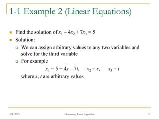
1-3 Definition
Two matrices are defined to be equal if they have the
same size and their corresponding entries are equal
If A = [aij] and B = [bij] have the same size, then A = B
if and only if aij = bij for all i and j
If A and B are matrices of the same size, then the sum A +
B is the matrix obtained by adding the entries of B to the
corresponding entries of A.](https://image.slidesharecdn.com/6640173-230301011852-b3e4429f/85/6640173-ppt-32-320.jpg)
![1-3 Definition
The difference A – B is the matrix obtained by subtracting
the entries of B from the corresponding entries of A
If A is any matrix and c is any scalar, then the product cA
is the matrix obtained by multiplying each entry of the
matrix A by c. The matrix cA is said to be the scalar
multiple of A
If A = [aij], then cAij = cAij = caij](https://image.slidesharecdn.com/6640173-230301011852-b3e4429f/85/6640173-ppt-33-320.jpg)
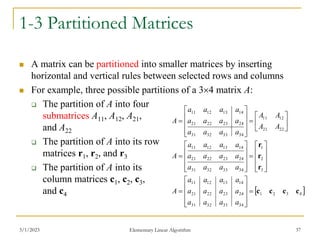
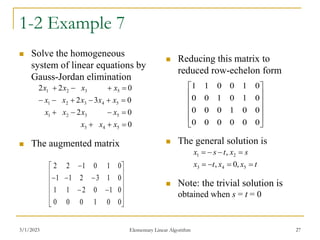
![3/1/2023 Elementary Linear Algorithm 38
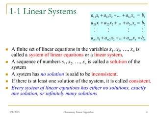
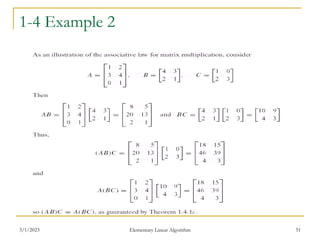
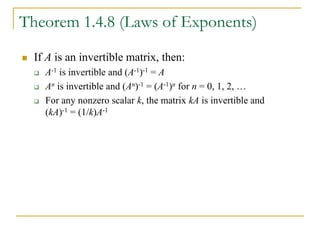
1-3 Multiplication by Columns and by Rows
It is possible to compute a particular row or column of a
matrix product AB without computing the entire product:
jth column matrix of AB = A[jth column matrix of B]
ith row matrix of AB = [ith row matrix of A]B
If a1, a2, ..., am denote the row matrices of A and b1 ,b2, ...,bn
denote the column matrices of B,then
B
B
B
B
AB
A
A
A
A
AB
m
m
n
n
a
a
a
a
a
a
b
b
b
b
b
b
2
1
2
1
2
1
2
1](https://image.slidesharecdn.com/6640173-230301011852-b3e4429f/85/6640173-ppt-38-320.jpg)
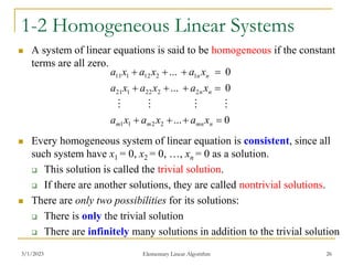
![3/1/2023 Elementary Linear Algorithm 45
1-3 Definitions
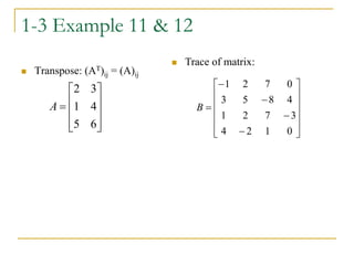
If A is any mn matrix, then the transpose of A, denoted
by AT, is defined to be the nm matrix that results from
interchanging the rows and columns of A
That is, the first column of AT is the first row of A, the second
column of AT is the second row of A, and so forth
If A is a square matrix, then the trace of A , denoted by
tr(A), is defined to be the sum of the entries on the main
diagonal of A. The trace of A is undefined if A is not a
square matrix.
For an nn matrix A = [aij],
n
i
ii
a
A
1
)
(
tr](https://image.slidesharecdn.com/6640173-230301011852-b3e4429f/85/6640173-ppt-45-320.jpg)
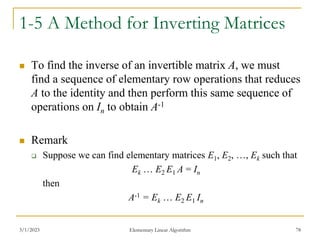
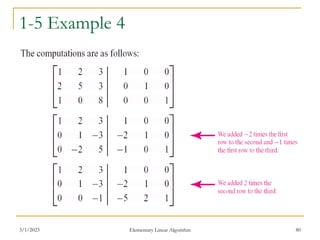
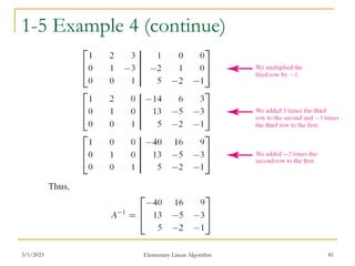
![3/1/2023 Elementary Linear Algorithm 79
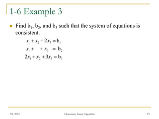
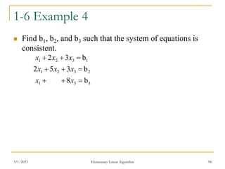
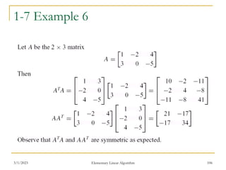
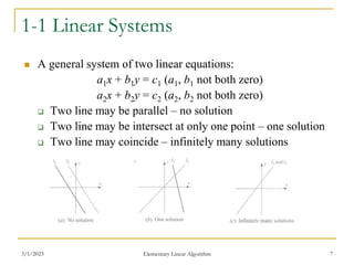
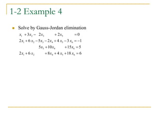
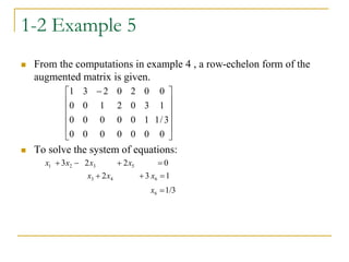
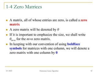
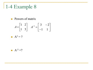
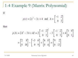
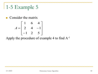
1-5 Example 4
(Using Row Operations to Find A-1)
Find the inverse of
Solution:
To accomplish this we shall adjoin the identity matrix to the right
side of A, thereby producing a matrix of the form [A | I]
We shall apply row operations to this matrix until the left side is
reduced to I; these operations will convert the right side to A-1, so
that the final matrix will have the form [I | A-1]
8
0
1
3
5
2
3
2
1
A](https://image.slidesharecdn.com/6640173-230301011852-b3e4429f/85/6640173-ppt-79-320.jpg)

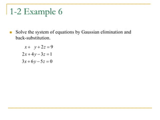
![3/1/2023 Elementary Linear Algorithm 88
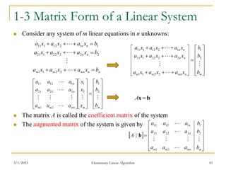
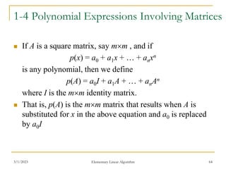
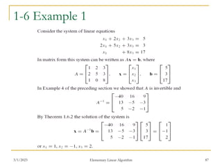
1-6 Linear Systems
with a Common Coefficient Matrix
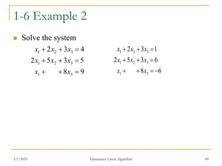
To solve a sequence of linear systems, Ax = b1, Ax = b1, …,
Ax = bk, with common coefficient matrix A
If A is invertible, then the solutions x1 = A-1b1, x2 = A-1b2 , …,
xk = A-1bk
A more efficient method is to form the matrix [A|b1|b2|…|bk]
By reducing it to reduced row-echelon form we can solve all k
systems at once by Gauss-Jordan elimination.](https://image.slidesharecdn.com/6640173-230301011852-b3e4429f/85/6640173-ppt-88-320.jpg)