Downloaded 59 times


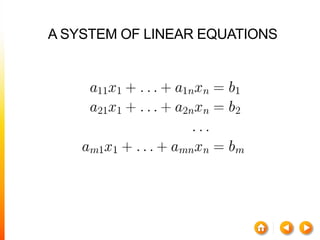

![A method to solve simultaneous linear
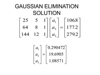
equations of the form [A][X]=[C]
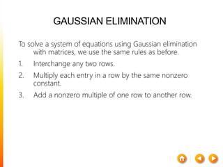
Two steps
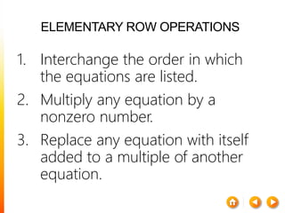
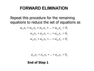
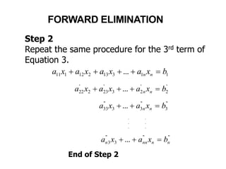
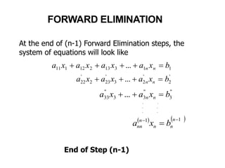
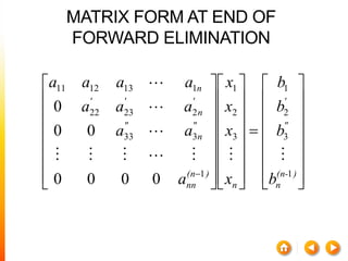
1. Forward Elimination
2. Back Substitution](https://image.slidesharecdn.com/dskmatrix-150412051806-conversion-gate01/85/Matrix-presentation-By-DHEERAJ-KATARIA-90-320.jpg)


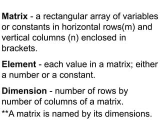
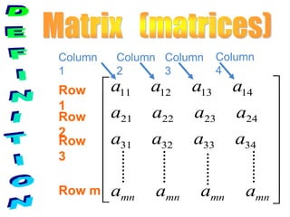
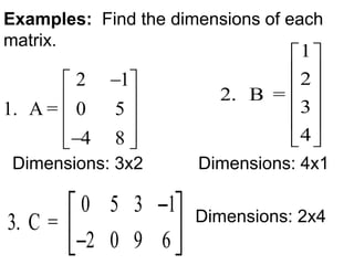
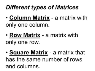
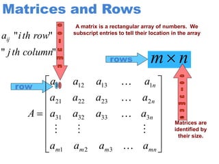
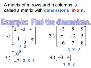
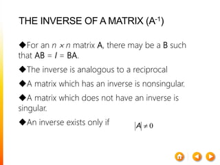
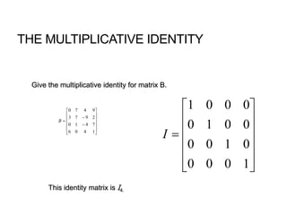
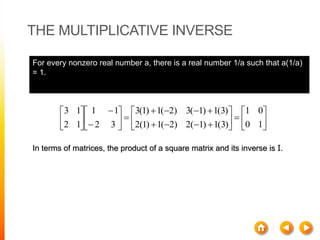
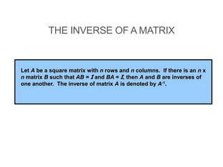
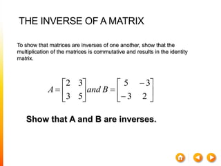
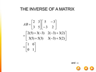
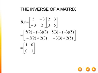
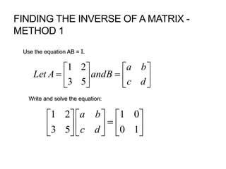
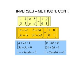
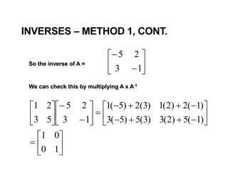
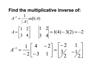
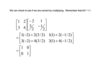
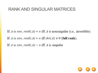
1) A matrix is a rectangular array of numbers arranged in rows and columns. The dimensions of a matrix are specified by the number of rows and columns. 2) The inverse of a square matrix A exists if and only if the determinant of A is not equal to 0. The inverse of A, denoted A^-1, is the matrix that satisfies AA^-1 = A^-1A = I, where I is the identity matrix. 3) For two matrices A and B to be inverses, their product must result in the identity matrix regardless of order, i.e. AB = BA = I. This shows that one matrix undoes the effect of the other.