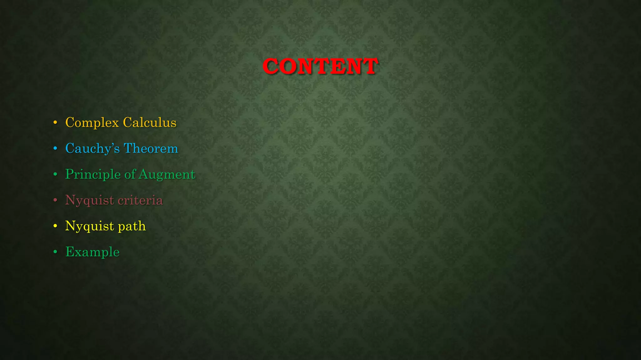
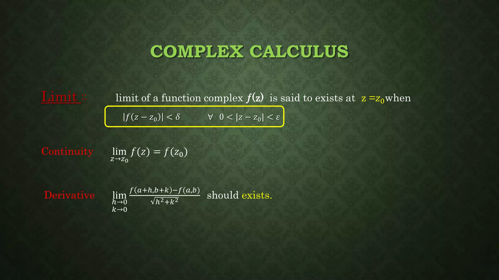
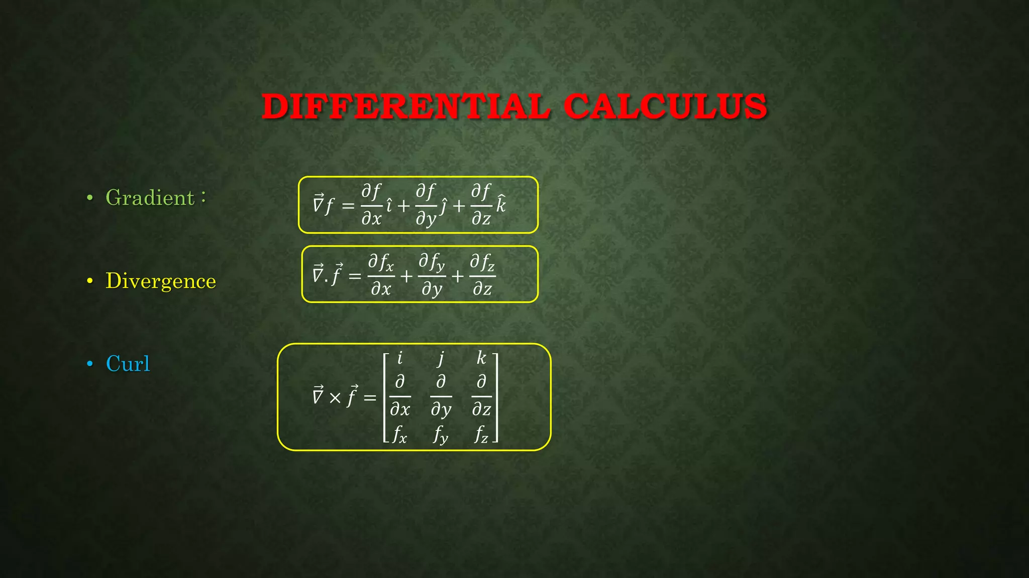
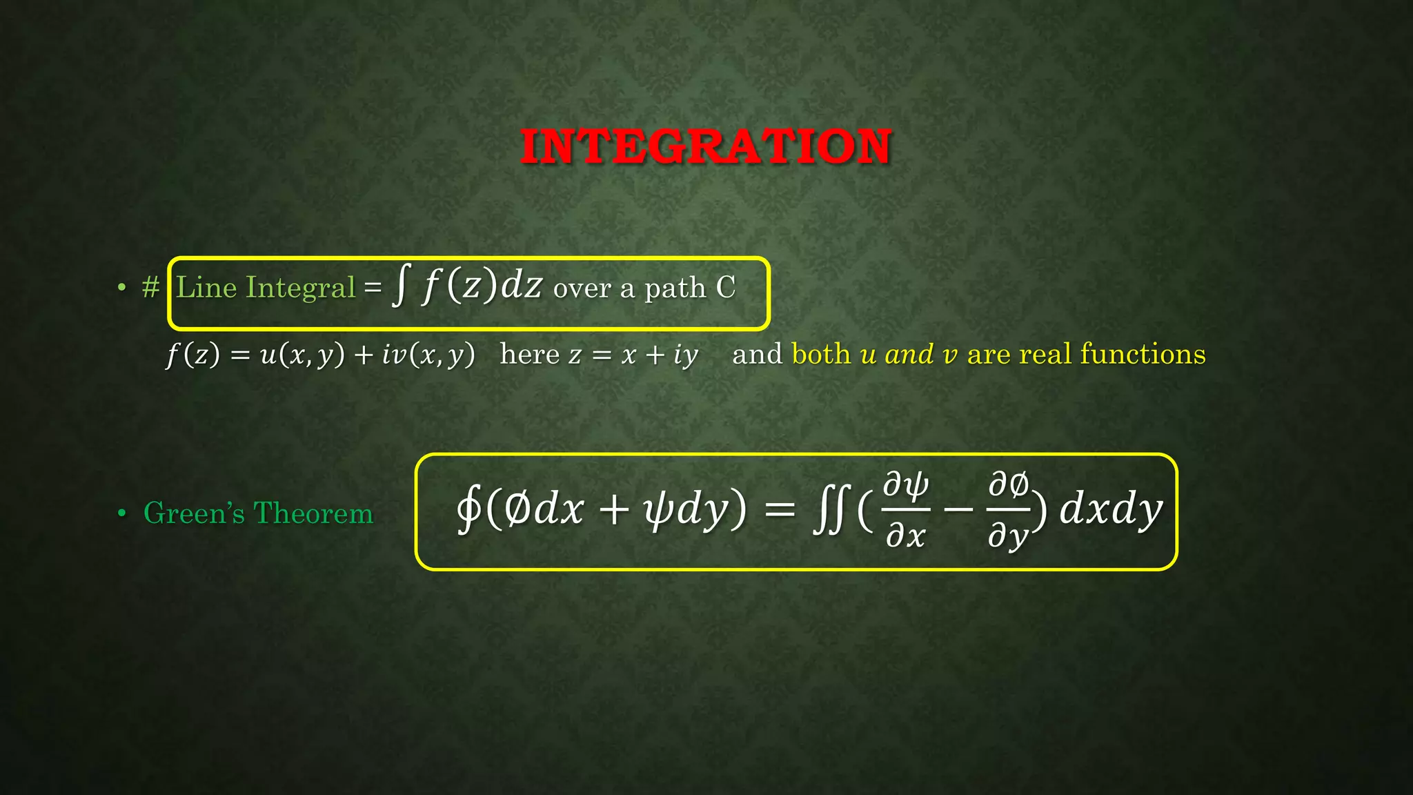
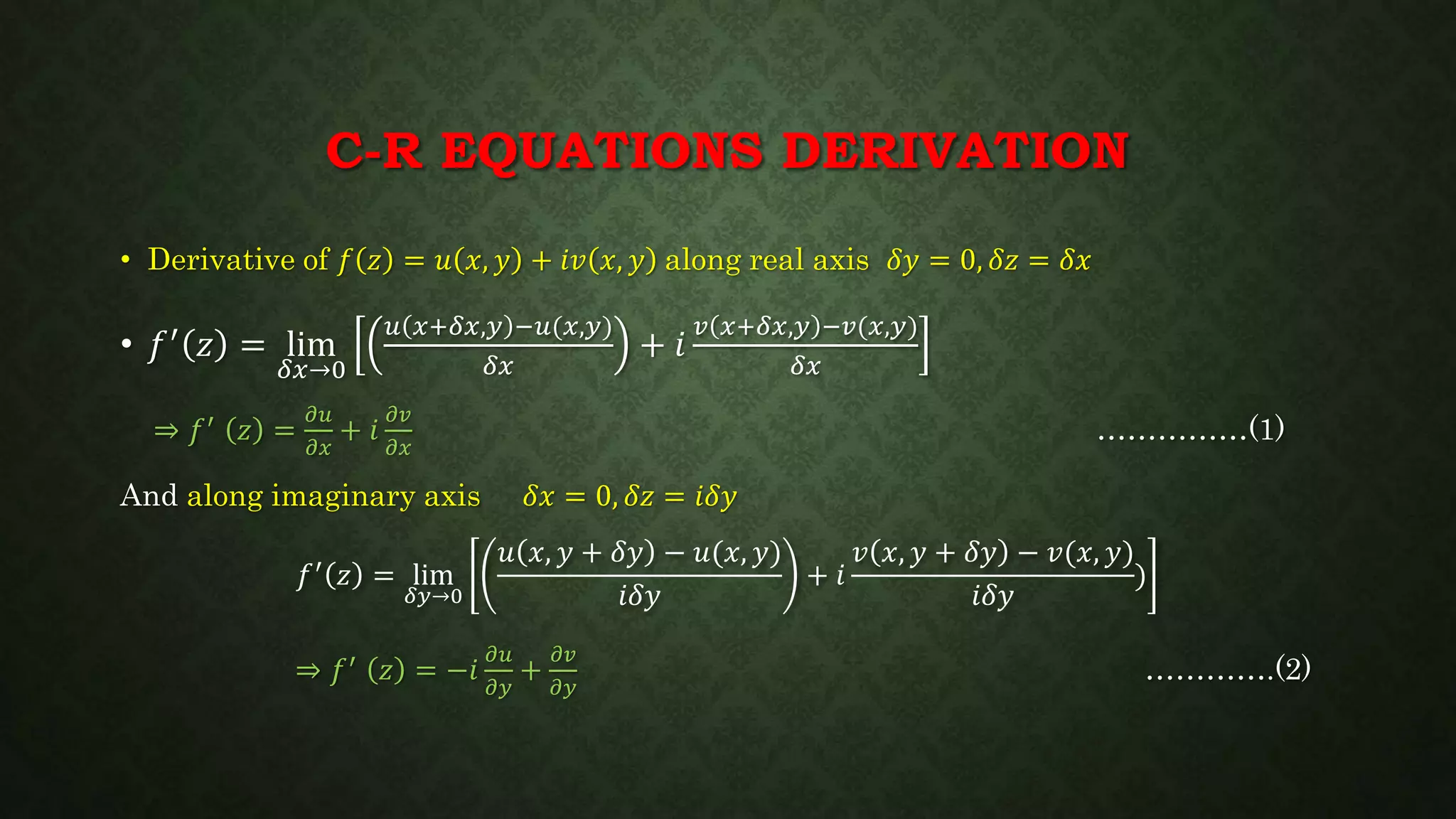
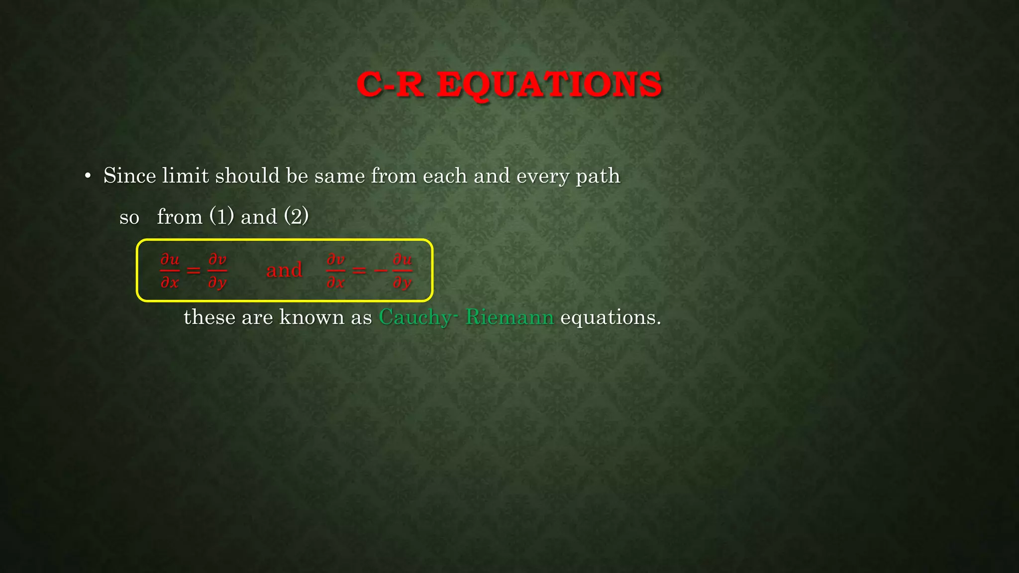
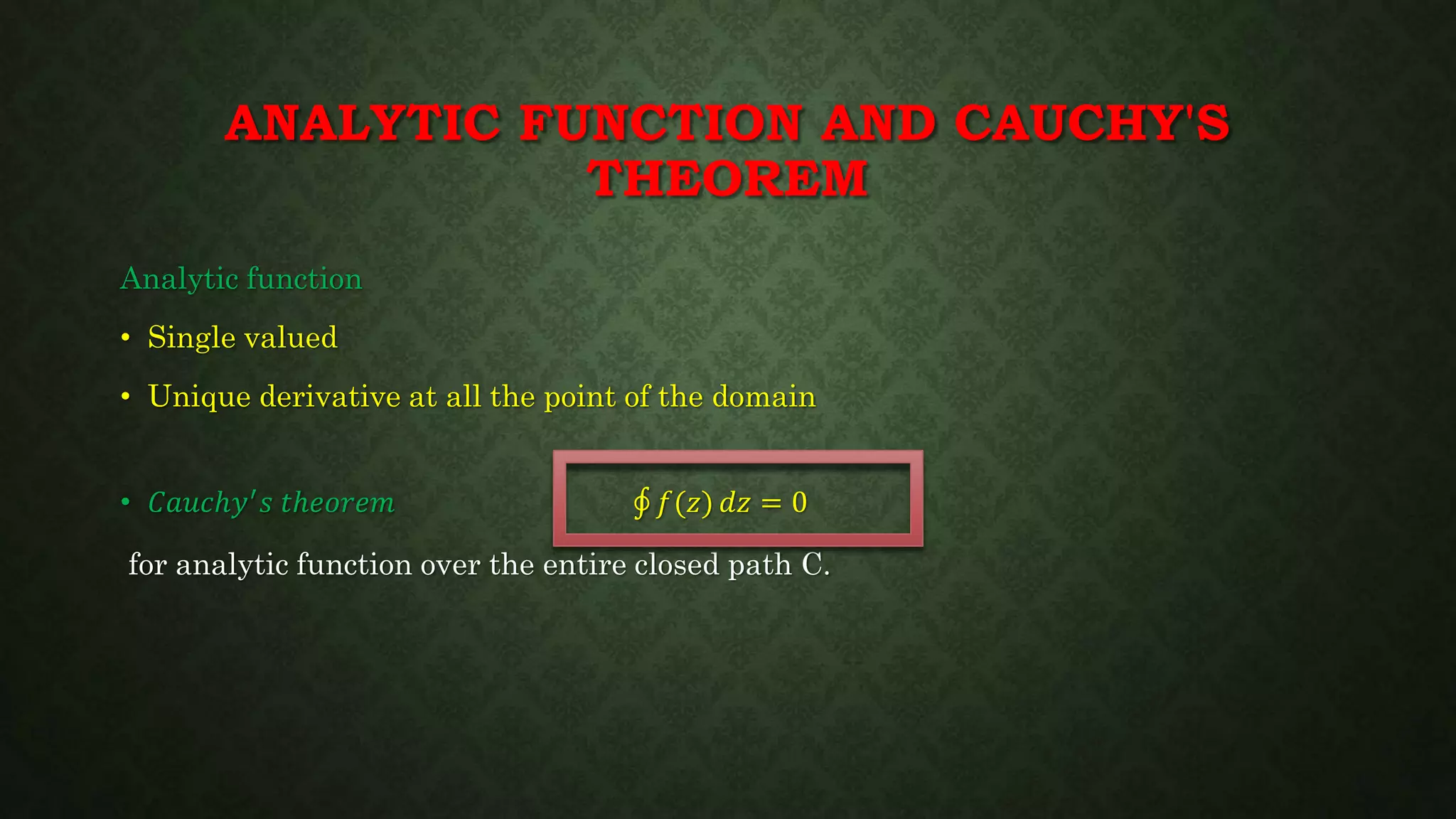
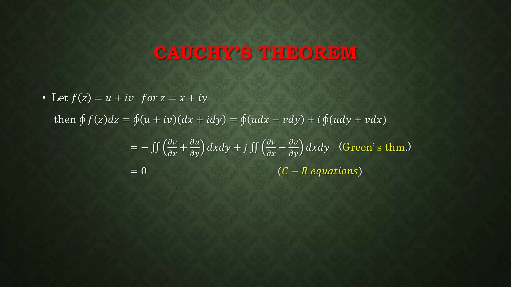
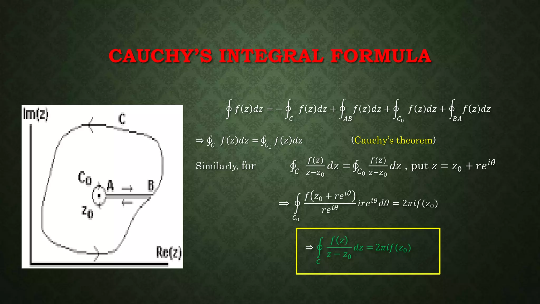
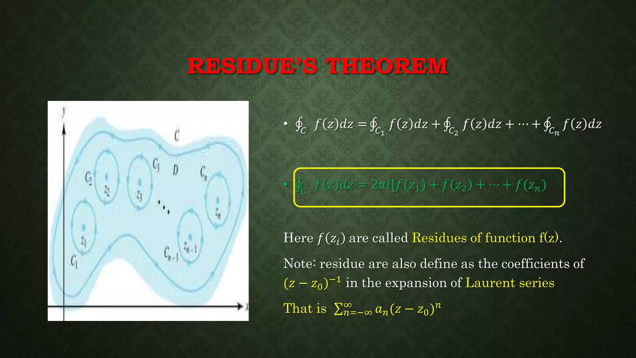
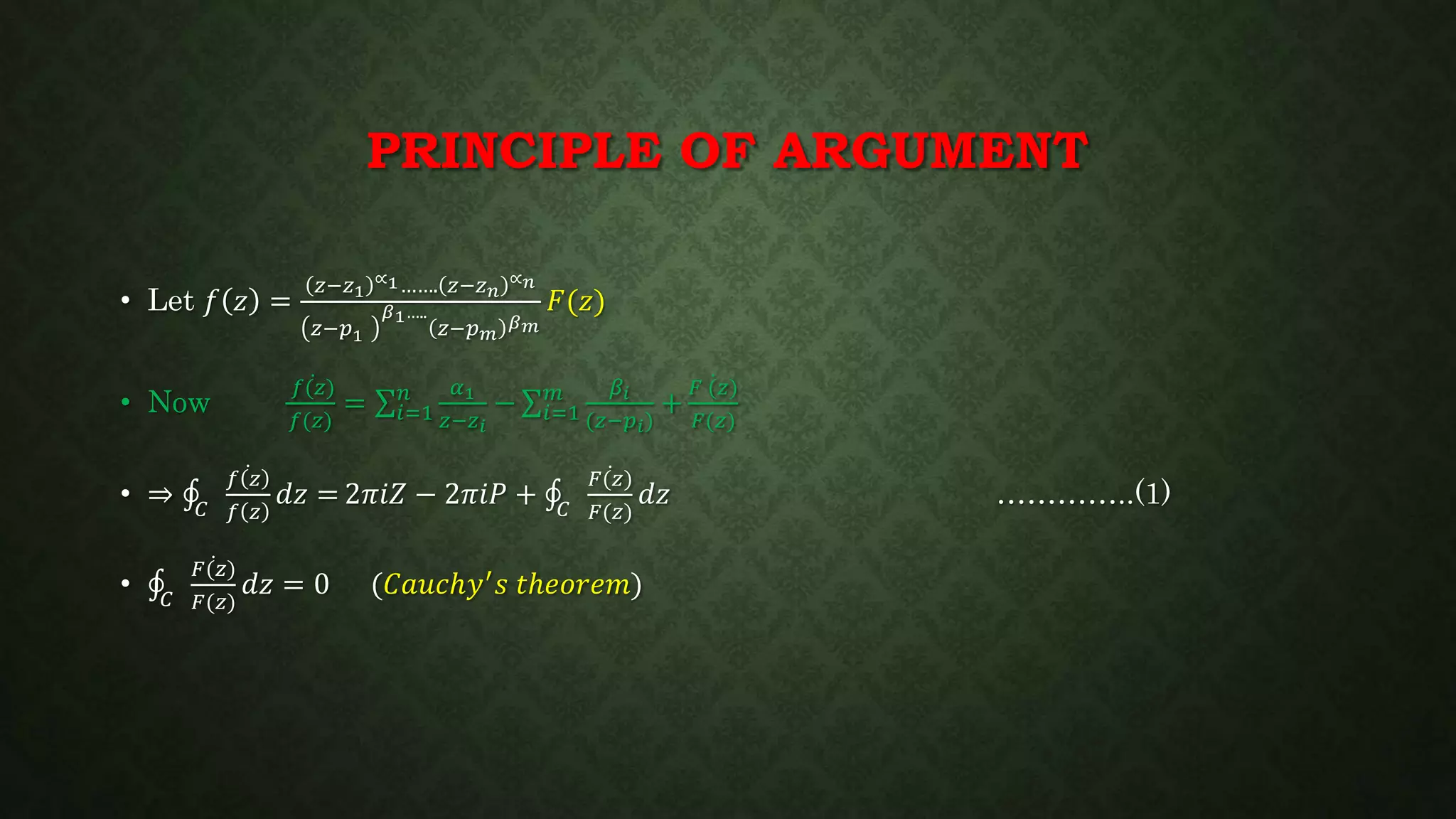
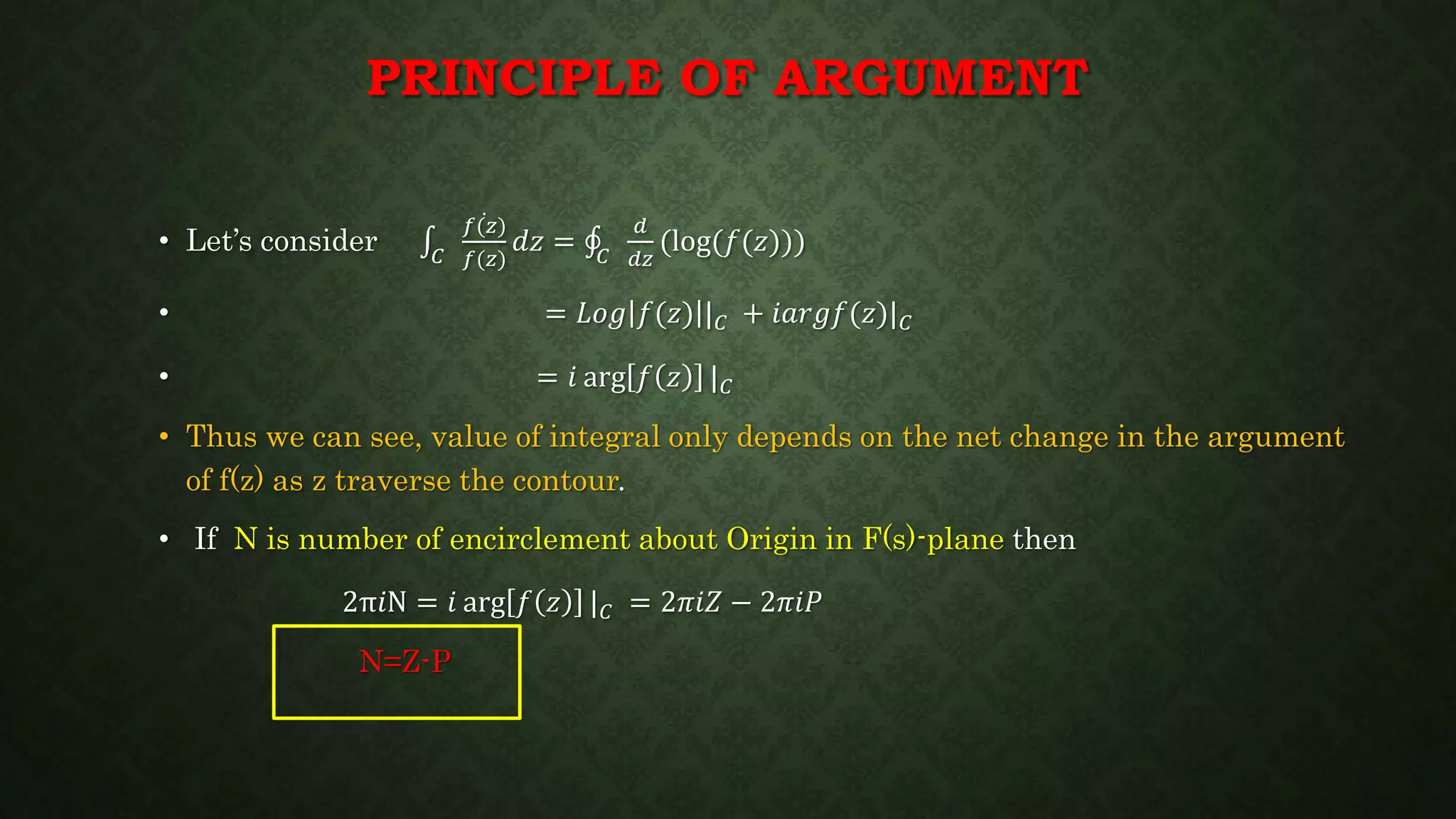
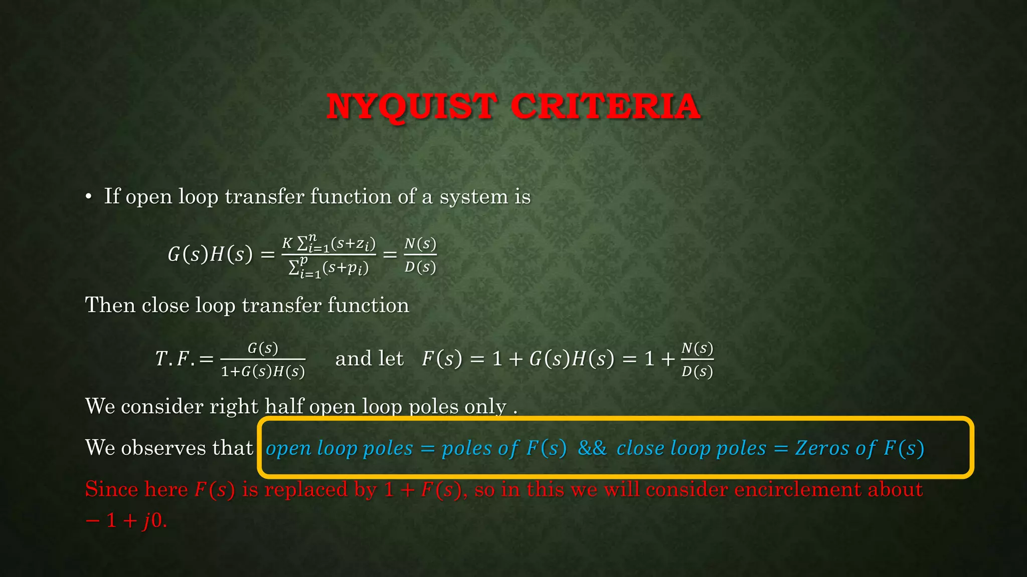
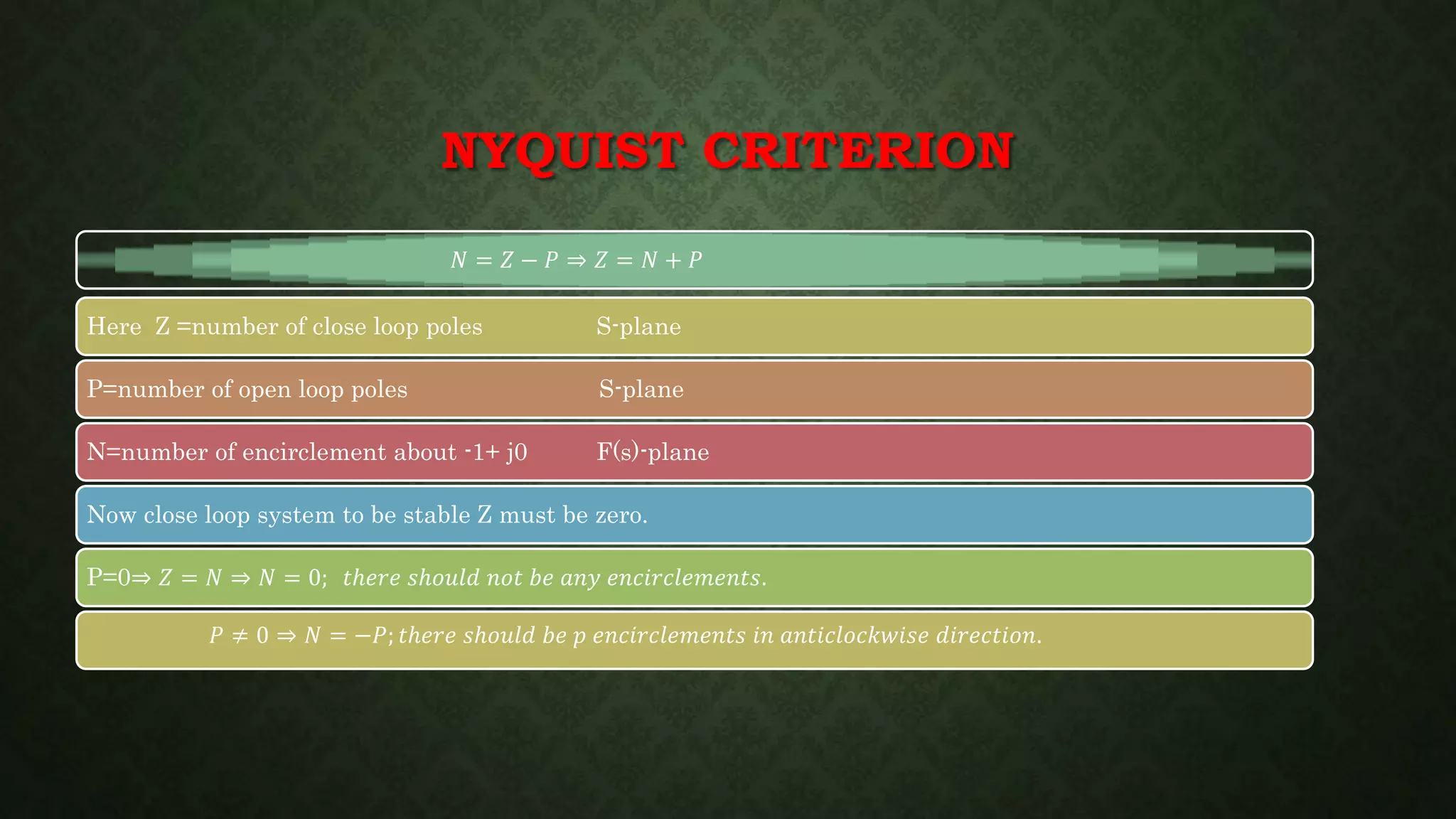
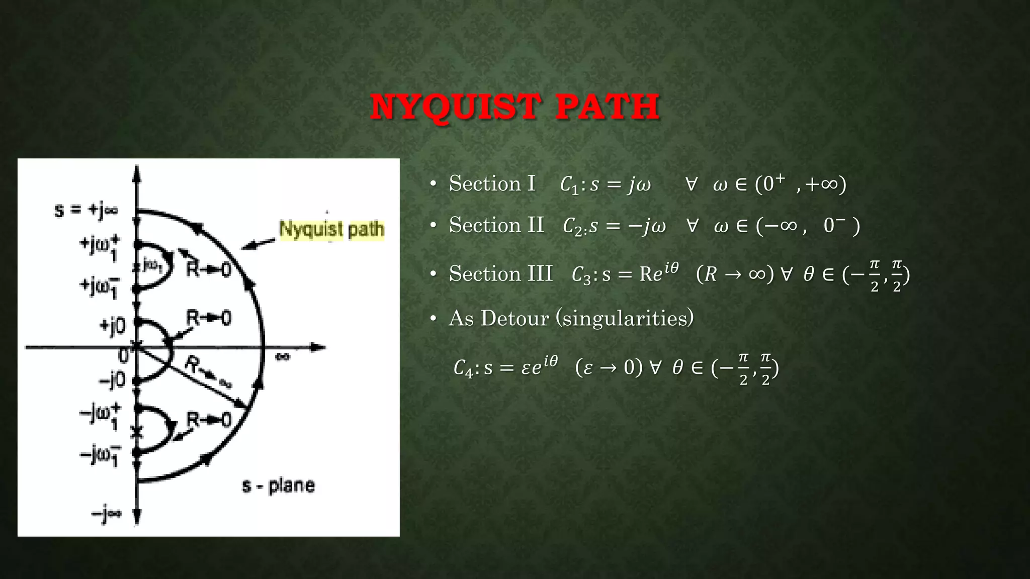
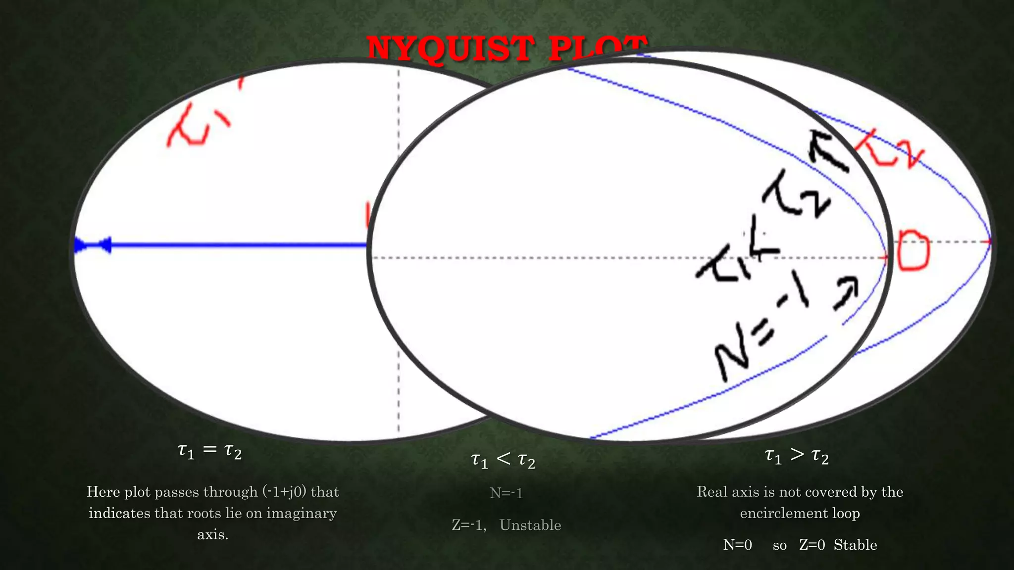
LECTURE-CUM-
PRESENTATION
ON
MATHEMATICS OF
NYQUIST PLOT
ASAFAK HUSAIN
12115026
E-2 BATCH, EE, 3rd year
CONTENT
• Complex Calculus
• Cauchy’s Theorem
• Principle of Augment
• Nyquist criteria
• Nyquist path
• Example
COMPLEX CALCULUS
Limit :: limit of a function complex ƒ(z) is said to exists at z =𝑧0when
𝑓 𝑧 − 𝑧0 < 𝛿 ∀ 0 < |𝑧 − 𝑧0| < 𝜀
Continuity lim
𝑧→𝑧0
𝑓(𝑧) = 𝑓(𝑧0)
Derivative lim
ℎ→0
𝑘→0
𝑓 𝑎+ℎ,𝑏+𝑘 −𝑓(𝑎,𝑏)
ℎ2+𝑘2
should exists.
DIFFERENTIAL CALCULUS
• Gradient :
• Divergence
• Curl
𝛻𝑓 =
𝜕𝑓
𝜕𝑥
𝑖 +
𝜕𝑓
𝜕𝑦
𝑗 +
𝜕𝑓
𝜕𝑧
𝑘
𝛻. 𝑓 =
𝜕𝑓𝑥
𝜕𝑥
+
𝜕𝑓𝑦
𝜕𝑦
+
𝜕𝑓𝑧
𝜕𝑧
𝛻 × 𝑓 =
𝑖 𝑗 𝑘
𝜕
𝜕𝑥
𝜕
𝜕𝑦
𝜕
𝜕𝑧
𝑓𝑥 𝑓𝑦 𝑓𝑧
INTEGRATION
• # Line Integral = 𝑓 𝑧 𝑑𝑧 over a path C
𝑓 𝑧 = 𝑢 𝑥, 𝑦 + 𝑖𝑣 𝑥, 𝑦 here 𝑧 = 𝑥 + 𝑖𝑦 and both 𝑢 𝑎𝑛𝑑 𝑣 are real functions
• Green’s Theorem ∅𝑑𝑥 + 𝜓𝑑𝑦 = (
𝜕𝜓
𝜕𝑥
−
𝜕∅
𝜕𝑦
) 𝑑𝑥𝑑𝑦
C-R EQUATIONS DERIVATION
• Derivative of 𝑓 𝑧 = 𝑢 𝑥, 𝑦 + 𝑖𝑣 𝑥, 𝑦 along real axis 𝛿𝑦 = 0, 𝛿𝑧 = 𝛿𝑥
• 𝑓′ 𝑧 = lim
𝛿𝑥→0
𝑢 𝑥+𝛿𝑥,𝑦 −𝑢(𝑥,𝑦)
𝛿𝑥
+ 𝑖
𝑣 𝑥+𝛿𝑥,𝑦 −𝑣(𝑥,𝑦)
𝛿𝑥
⇒ 𝑓′ 𝑧 =
𝜕𝑢
𝜕𝑥
+ 𝑖
𝜕𝑣
𝜕𝑥
……………(1)
And along imaginary axis 𝛿𝑥 = 0, 𝛿𝑧 = 𝑖𝛿𝑦
𝑓′ 𝑧 = lim
𝛿𝑦→0
𝑢 𝑥, 𝑦 + 𝛿𝑦 − 𝑢(𝑥, 𝑦)
𝑖𝛿𝑦
+ 𝑖
𝑣 𝑥, 𝑦 + 𝛿𝑦 − 𝑣(𝑥, 𝑦)
𝑖𝛿𝑦
)
⇒ 𝑓′ 𝑧 = −𝑖
𝜕𝑢
𝜕𝑦
+
𝜕𝑣
𝜕𝑦
………….(2)
C-R EQUATIONS
• Since limit should be same from each and every path
so from (1) and (2)
𝜕𝑢
𝜕𝑥
=
𝜕𝑣
𝜕𝑦
and
𝜕𝑣
𝜕𝑥
= −
𝜕𝑢
𝜕𝑦
these are known as Cauchy- Riemann equations.
ANALYTIC FUNCTION AND CAUCHY'S
THEOREM
Analytic function
• Single valued
• Unique derivative at all the point of the domain
• 𝐶𝑎𝑢𝑐ℎ𝑦′ 𝑠 𝑡ℎ𝑒𝑜𝑟𝑒𝑚 𝑓(𝑧) 𝑑𝑧 = 0
for analytic function over the entire closed path C.
CAUCHY’S THEOREM
• Let 𝑓 𝑧 = 𝑢 + 𝑖𝑣 𝑓𝑜𝑟 𝑧 = 𝑥 + 𝑖𝑦
then 𝑓 𝑧 𝑑𝑧 = 𝑢 + 𝑖𝑣 𝑑𝑥 + 𝑖𝑑𝑦 = 𝑢𝑑𝑥 − 𝑣𝑑𝑦 + 𝑖 (𝑢𝑑𝑦 + 𝑣𝑑𝑥)
= −
𝜕𝑣
𝜕𝑥
+
𝜕𝑢
𝜕𝑦
𝑑𝑥𝑑𝑦 + 𝑗
𝜕𝑣
𝜕𝑥
−
𝜕𝑢
𝜕𝑦
𝑑𝑥𝑑𝑦 (Green’ s thm.)
= 0 (𝐶 − 𝑅 𝑒𝑞𝑢𝑎𝑡𝑖𝑜𝑛𝑠)
CAUCHY’S INTEGRAL FORMULA
𝑓 𝑧 𝑑𝑧 = −
𝐶
𝑓 𝑧 𝑑𝑧 +
𝐴𝐵
𝑓 𝑧 𝑑𝑧 +
𝐶0
𝑓 𝑧 𝑑𝑧 +
𝐵𝐴
𝑓 𝑧 𝑑𝑧
⇒ 𝐶
𝑓 𝑧 𝑑𝑧 = 𝐶1
𝑓 𝑧 𝑑𝑧 (Cauchy’s theorem)
Similarly, for 𝐶
𝑓(𝑧)
𝑧−𝑧0
𝑑𝑧 = 𝐶0
𝑓(𝑧)
𝑧−𝑧0
𝑑𝑧 , put 𝑧 = 𝑧0 + 𝑟𝑒 𝑖𝜃
⟹
𝐶0
𝑓 𝑧0 + 𝑟𝑒 𝑖𝜃
𝑟𝑒 𝑖𝜃
𝑖𝑟𝑒 𝑖𝜃 𝑑𝜃 = 2𝜋𝑖𝑓(𝑧0)
⇒
𝐶
𝑓 𝑧
𝑧 − 𝑧0
𝑑𝑧 = 2𝜋𝑖𝑓(𝑧0)
RESIDUE’S THEOREM
• 𝐶
𝑓 𝑧 𝑑𝑧 = 𝐶1
𝑓 𝑧 𝑑𝑧 + 𝐶2
𝑓 𝑧 𝑑𝑧 + ⋯ + 𝐶 𝑛
𝑓 𝑧 𝑑𝑧
• 𝐶
𝑓 𝑧 𝑑𝑧 = 2𝜋𝑖[𝑓(𝑧1) + 𝑓 𝑧2 + ⋯ + 𝑓(𝑧 𝑛)
Here 𝑓 𝑧𝑖 are called Residues of function f(z).
Note: residue are also define as the coefficients of
(𝑧 − 𝑧0)−1 in the expansion of Laurent series
That is 𝑛=−∞
∞
𝑎 𝑛(𝑧 − 𝑧0) 𝑛
PRINCIPLE OF ARGUMENT
• Let 𝑓 𝑧 =
𝑧−𝑧1
∝1……. 𝑧−𝑧 𝑛
∝ 𝑛
𝑧−𝑝1
𝛽1…..
𝑧−𝑝 𝑚
𝛽 𝑚
𝐹(𝑧)
• Now
𝑓(𝑧)
𝑓(𝑧)
= 𝑖=1
𝑛 𝛼1
𝑧−𝑧 𝑖
− 𝑖=1
𝑚 𝛽𝑖
(𝑧−𝑝 𝑖)
+
𝐹 (𝑧)
𝐹(𝑧)
• ⇒ 𝐶
𝑓 𝑧
𝑓 𝑧
𝑑𝑧 = 2𝜋𝑖𝑍 − 2𝜋𝑖𝑃 + 𝐶
𝐹(𝑧)
𝐹(𝑧)
𝑑𝑧 …………..(1)
• 𝐶
𝐹(𝑧)
𝐹(𝑧)
𝑑𝑧 = 0 (𝐶𝑎𝑢𝑐ℎ𝑦′ 𝑠 𝑡ℎ𝑒𝑜𝑟𝑒𝑚)
PRINCIPLE OF ARGUMENT
• Let’s consider 𝐶
𝑓(𝑧)
𝑓(𝑧)
𝑑𝑧 = 𝐶
𝑑
𝑑𝑧
(log(𝑓(𝑧)))
• = 𝐿𝑜𝑔 𝑓(𝑧) | 𝐶 + 𝑖𝑎𝑟𝑔𝑓(𝑧)| 𝐶
• = 𝑖 arg 𝑓 𝑧 | 𝐶
• Thus we can see, value of integral only depends on the net change in the argument
of f(z) as z traverse the contour.
• If N is number of encirclement about Origin in F(s)-plane then
2π𝑖N = 𝑖 arg 𝑓 𝑧 | 𝐶 = 2𝜋𝑖𝑍 − 2𝜋𝑖𝑃
N=Z-P
NYQUIST CRITERIA
• If open loop transfer function of a system is
𝐺 𝑠 𝐻 𝑠 =
𝐾 𝑖=1
𝑛
(𝑠+𝑧 𝑖)
𝑖=1
𝑝
(𝑠+𝑝 𝑖)
=
𝑁(𝑠)
𝐷(𝑠)
Then close loop transfer function
𝑇. 𝐹. =
𝐺(𝑠)
1+𝐺 𝑠 𝐻(𝑠)
and let 𝐹 𝑠 = 1 + 𝐺 𝑠 𝐻 𝑠 = 1 +
𝑁(𝑠)
𝐷(𝑠)
We consider right half open loop poles only .
We observes that 𝑜𝑝𝑒𝑛 𝑙𝑜𝑜𝑝 𝑝𝑜𝑙𝑒𝑠 = 𝑝𝑜𝑙𝑒𝑠 𝑜𝑓 𝐹 𝑠 && 𝑐𝑙𝑜𝑠𝑒 𝑙𝑜𝑜𝑝 𝑝𝑜𝑙𝑒𝑠 = 𝑍𝑒𝑟𝑜𝑠 𝑜𝑓 𝐹(𝑠)
Since here 𝐹(𝑠) is replaced by 1 + 𝐹(𝑠), so in this we will consider encirclement about
− 1 + 𝑗0.
NYQUIST CRITERION
𝑁 = 𝑍 − 𝑃 ⇒ 𝑍 = 𝑁 + 𝑃
Here Z =number of close loop poles S-plane
P=number of open loop poles S-plane
N=number of encirclement about -1+ j0 F(s)-plane
Now close loop system to be stable Z must be zero.
P=0⇒ 𝑍 = 𝑁 ⇒ 𝑁 = 0; 𝑡ℎ𝑒𝑟𝑒 𝑠ℎ𝑜𝑢𝑙𝑑 𝑛𝑜𝑡 𝑏𝑒 𝑎𝑛𝑦 𝑒𝑛𝑐𝑖𝑟𝑐𝑙𝑒𝑚𝑒𝑛𝑡𝑠.
𝑃 ≠ 0 ⇒ 𝑁 = −𝑃; 𝑡ℎ𝑒𝑟𝑒 𝑠ℎ𝑜𝑢𝑙𝑑 𝑏𝑒 𝑝 𝑒𝑛𝑐𝑖𝑟𝑐𝑙𝑒𝑚𝑒𝑛𝑡𝑠 𝑖𝑛 𝑎𝑛𝑡𝑖𝑐𝑙𝑜𝑐𝑘𝑤𝑖𝑠𝑒 𝑑𝑖𝑟𝑒𝑐𝑡𝑖𝑜𝑛.
NYQUIST PATH
• Section I 𝐶1: 𝑠 = 𝑗𝜔 ∀ 𝜔 ∈ (0+
, +∞)
• Section II 𝐶2∶ 𝑠 = −𝑗𝜔 ∀ 𝜔 ∈ (−∞ , 0− )
• Section III 𝐶3: s = R𝑒 𝑖𝜃 𝑅 → ∞ ∀ 𝜃 ∈ (−
𝜋
2
,
𝜋
2
)
• As Detour (singularities)
𝐶4: s = 𝜀𝑒 𝑖𝜃 𝜀 → 0 ∀ 𝜃 ∈ (−
𝜋
2
,
𝜋
2
)
EXAMPLE
• Section 𝐶3:
• 𝐺 𝑅𝑒 𝑗𝜃
𝐻 𝑅𝑒 𝑗𝜃
= 0
• At detour
• 𝐺 𝜀𝑒 𝑗𝜃
𝐻 𝜀𝑒 𝑗𝜃
→ ∞
• 𝐺 𝑠 𝐻 𝑠 =
𝐾(𝜏1 𝑠+1)
𝑠2(𝜏2 𝑠+1)
, find close loop
stability of the system.
• (1) Section 𝐶1& 𝐶2
• 𝐺 𝑗𝜔 𝐻 𝑗𝜔 =
𝐾
𝜔2
𝜏1 𝜔 2+1
𝜏2 𝜔 2+1
𝜑 𝐺𝐻 = −𝜋 + tan−1
𝜏1 𝜔 − tan−1
𝜏2 𝜔
NYQUIST PLOT
𝜏1 = 𝜏2
Here plot passes through (-1+j0) that
indicates that roots lie on imaginary
axis.
𝜏1 < 𝜏2
N=-1
Z=-1, Unstable
𝜏1 > 𝜏2
Real axis is not covered by the
encirclement loop
N=0 so Z=0 Stable
THANKS A LOT !!!!!!!!!!!!!!!
Any queries ??????

Mathematics of nyquist plot [autosaved] [autosaved]

  • 1.
  • 2.
    CONTENT • Complex Calculus •Cauchy’s Theorem • Principle of Augment • Nyquist criteria • Nyquist path • Example
  • 3.
    COMPLEX CALCULUS Limit ::limit of a function complex ƒ(z) is said to exists at z =𝑧0when 𝑓 𝑧 − 𝑧0 < 𝛿 ∀ 0 < |𝑧 − 𝑧0| < 𝜀 Continuity lim 𝑧→𝑧0 𝑓(𝑧) = 𝑓(𝑧0) Derivative lim ℎ→0 𝑘→0 𝑓 𝑎+ℎ,𝑏+𝑘 −𝑓(𝑎,𝑏) ℎ2+𝑘2 should exists.
  • 4.
    DIFFERENTIAL CALCULUS • Gradient: • Divergence • Curl 𝛻𝑓 = 𝜕𝑓 𝜕𝑥 𝑖 + 𝜕𝑓 𝜕𝑦 𝑗 + 𝜕𝑓 𝜕𝑧 𝑘 𝛻. 𝑓 = 𝜕𝑓𝑥 𝜕𝑥 + 𝜕𝑓𝑦 𝜕𝑦 + 𝜕𝑓𝑧 𝜕𝑧 𝛻 × 𝑓 = 𝑖 𝑗 𝑘 𝜕 𝜕𝑥 𝜕 𝜕𝑦 𝜕 𝜕𝑧 𝑓𝑥 𝑓𝑦 𝑓𝑧
  • 5.
    INTEGRATION • # LineIntegral = 𝑓 𝑧 𝑑𝑧 over a path C 𝑓 𝑧 = 𝑢 𝑥, 𝑦 + 𝑖𝑣 𝑥, 𝑦 here 𝑧 = 𝑥 + 𝑖𝑦 and both 𝑢 𝑎𝑛𝑑 𝑣 are real functions • Green’s Theorem ∅𝑑𝑥 + 𝜓𝑑𝑦 = ( 𝜕𝜓 𝜕𝑥 − 𝜕∅ 𝜕𝑦 ) 𝑑𝑥𝑑𝑦
  • 6.
    C-R EQUATIONS DERIVATION •Derivative of 𝑓 𝑧 = 𝑢 𝑥, 𝑦 + 𝑖𝑣 𝑥, 𝑦 along real axis 𝛿𝑦 = 0, 𝛿𝑧 = 𝛿𝑥 • 𝑓′ 𝑧 = lim 𝛿𝑥→0 𝑢 𝑥+𝛿𝑥,𝑦 −𝑢(𝑥,𝑦) 𝛿𝑥 + 𝑖 𝑣 𝑥+𝛿𝑥,𝑦 −𝑣(𝑥,𝑦) 𝛿𝑥 ⇒ 𝑓′ 𝑧 = 𝜕𝑢 𝜕𝑥 + 𝑖 𝜕𝑣 𝜕𝑥 ……………(1) And along imaginary axis 𝛿𝑥 = 0, 𝛿𝑧 = 𝑖𝛿𝑦 𝑓′ 𝑧 = lim 𝛿𝑦→0 𝑢 𝑥, 𝑦 + 𝛿𝑦 − 𝑢(𝑥, 𝑦) 𝑖𝛿𝑦 + 𝑖 𝑣 𝑥, 𝑦 + 𝛿𝑦 − 𝑣(𝑥, 𝑦) 𝑖𝛿𝑦 ) ⇒ 𝑓′ 𝑧 = −𝑖 𝜕𝑢 𝜕𝑦 + 𝜕𝑣 𝜕𝑦 ………….(2)
  • 7.
    C-R EQUATIONS • Sincelimit should be same from each and every path so from (1) and (2) 𝜕𝑢 𝜕𝑥 = 𝜕𝑣 𝜕𝑦 and 𝜕𝑣 𝜕𝑥 = − 𝜕𝑢 𝜕𝑦 these are known as Cauchy- Riemann equations.
  • 8.
    ANALYTIC FUNCTION ANDCAUCHY'S THEOREM Analytic function • Single valued • Unique derivative at all the point of the domain • 𝐶𝑎𝑢𝑐ℎ𝑦′ 𝑠 𝑡ℎ𝑒𝑜𝑟𝑒𝑚 𝑓(𝑧) 𝑑𝑧 = 0 for analytic function over the entire closed path C.
  • 9.
    CAUCHY’S THEOREM • Let𝑓 𝑧 = 𝑢 + 𝑖𝑣 𝑓𝑜𝑟 𝑧 = 𝑥 + 𝑖𝑦 then 𝑓 𝑧 𝑑𝑧 = 𝑢 + 𝑖𝑣 𝑑𝑥 + 𝑖𝑑𝑦 = 𝑢𝑑𝑥 − 𝑣𝑑𝑦 + 𝑖 (𝑢𝑑𝑦 + 𝑣𝑑𝑥) = − 𝜕𝑣 𝜕𝑥 + 𝜕𝑢 𝜕𝑦 𝑑𝑥𝑑𝑦 + 𝑗 𝜕𝑣 𝜕𝑥 − 𝜕𝑢 𝜕𝑦 𝑑𝑥𝑑𝑦 (Green’ s thm.) = 0 (𝐶 − 𝑅 𝑒𝑞𝑢𝑎𝑡𝑖𝑜𝑛𝑠)
  • 10.
    CAUCHY’S INTEGRAL FORMULA 𝑓𝑧 𝑑𝑧 = − 𝐶 𝑓 𝑧 𝑑𝑧 + 𝐴𝐵 𝑓 𝑧 𝑑𝑧 + 𝐶0 𝑓 𝑧 𝑑𝑧 + 𝐵𝐴 𝑓 𝑧 𝑑𝑧 ⇒ 𝐶 𝑓 𝑧 𝑑𝑧 = 𝐶1 𝑓 𝑧 𝑑𝑧 (Cauchy’s theorem) Similarly, for 𝐶 𝑓(𝑧) 𝑧−𝑧0 𝑑𝑧 = 𝐶0 𝑓(𝑧) 𝑧−𝑧0 𝑑𝑧 , put 𝑧 = 𝑧0 + 𝑟𝑒 𝑖𝜃 ⟹ 𝐶0 𝑓 𝑧0 + 𝑟𝑒 𝑖𝜃 𝑟𝑒 𝑖𝜃 𝑖𝑟𝑒 𝑖𝜃 𝑑𝜃 = 2𝜋𝑖𝑓(𝑧0) ⇒ 𝐶 𝑓 𝑧 𝑧 − 𝑧0 𝑑𝑧 = 2𝜋𝑖𝑓(𝑧0)
  • 11.
    RESIDUE’S THEOREM • 𝐶 𝑓𝑧 𝑑𝑧 = 𝐶1 𝑓 𝑧 𝑑𝑧 + 𝐶2 𝑓 𝑧 𝑑𝑧 + ⋯ + 𝐶 𝑛 𝑓 𝑧 𝑑𝑧 • 𝐶 𝑓 𝑧 𝑑𝑧 = 2𝜋𝑖[𝑓(𝑧1) + 𝑓 𝑧2 + ⋯ + 𝑓(𝑧 𝑛) Here 𝑓 𝑧𝑖 are called Residues of function f(z). Note: residue are also define as the coefficients of (𝑧 − 𝑧0)−1 in the expansion of Laurent series That is 𝑛=−∞ ∞ 𝑎 𝑛(𝑧 − 𝑧0) 𝑛
  • 12.
    PRINCIPLE OF ARGUMENT •Let 𝑓 𝑧 = 𝑧−𝑧1 ∝1……. 𝑧−𝑧 𝑛 ∝ 𝑛 𝑧−𝑝1 𝛽1….. 𝑧−𝑝 𝑚 𝛽 𝑚 𝐹(𝑧) • Now 𝑓(𝑧) 𝑓(𝑧) = 𝑖=1 𝑛 𝛼1 𝑧−𝑧 𝑖 − 𝑖=1 𝑚 𝛽𝑖 (𝑧−𝑝 𝑖) + 𝐹 (𝑧) 𝐹(𝑧) • ⇒ 𝐶 𝑓 𝑧 𝑓 𝑧 𝑑𝑧 = 2𝜋𝑖𝑍 − 2𝜋𝑖𝑃 + 𝐶 𝐹(𝑧) 𝐹(𝑧) 𝑑𝑧 …………..(1) • 𝐶 𝐹(𝑧) 𝐹(𝑧) 𝑑𝑧 = 0 (𝐶𝑎𝑢𝑐ℎ𝑦′ 𝑠 𝑡ℎ𝑒𝑜𝑟𝑒𝑚)
  • 13.
    PRINCIPLE OF ARGUMENT •Let’s consider 𝐶 𝑓(𝑧) 𝑓(𝑧) 𝑑𝑧 = 𝐶 𝑑 𝑑𝑧 (log(𝑓(𝑧))) • = 𝐿𝑜𝑔 𝑓(𝑧) | 𝐶 + 𝑖𝑎𝑟𝑔𝑓(𝑧)| 𝐶 • = 𝑖 arg 𝑓 𝑧 | 𝐶 • Thus we can see, value of integral only depends on the net change in the argument of f(z) as z traverse the contour. • If N is number of encirclement about Origin in F(s)-plane then 2π𝑖N = 𝑖 arg 𝑓 𝑧 | 𝐶 = 2𝜋𝑖𝑍 − 2𝜋𝑖𝑃 N=Z-P
  • 14.
    NYQUIST CRITERIA • Ifopen loop transfer function of a system is 𝐺 𝑠 𝐻 𝑠 = 𝐾 𝑖=1 𝑛 (𝑠+𝑧 𝑖) 𝑖=1 𝑝 (𝑠+𝑝 𝑖) = 𝑁(𝑠) 𝐷(𝑠) Then close loop transfer function 𝑇. 𝐹. = 𝐺(𝑠) 1+𝐺 𝑠 𝐻(𝑠) and let 𝐹 𝑠 = 1 + 𝐺 𝑠 𝐻 𝑠 = 1 + 𝑁(𝑠) 𝐷(𝑠) We consider right half open loop poles only . We observes that 𝑜𝑝𝑒𝑛 𝑙𝑜𝑜𝑝 𝑝𝑜𝑙𝑒𝑠 = 𝑝𝑜𝑙𝑒𝑠 𝑜𝑓 𝐹 𝑠 && 𝑐𝑙𝑜𝑠𝑒 𝑙𝑜𝑜𝑝 𝑝𝑜𝑙𝑒𝑠 = 𝑍𝑒𝑟𝑜𝑠 𝑜𝑓 𝐹(𝑠) Since here 𝐹(𝑠) is replaced by 1 + 𝐹(𝑠), so in this we will consider encirclement about − 1 + 𝑗0.
  • 15.
    NYQUIST CRITERION 𝑁 =𝑍 − 𝑃 ⇒ 𝑍 = 𝑁 + 𝑃 Here Z =number of close loop poles S-plane P=number of open loop poles S-plane N=number of encirclement about -1+ j0 F(s)-plane Now close loop system to be stable Z must be zero. P=0⇒ 𝑍 = 𝑁 ⇒ 𝑁 = 0; 𝑡ℎ𝑒𝑟𝑒 𝑠ℎ𝑜𝑢𝑙𝑑 𝑛𝑜𝑡 𝑏𝑒 𝑎𝑛𝑦 𝑒𝑛𝑐𝑖𝑟𝑐𝑙𝑒𝑚𝑒𝑛𝑡𝑠. 𝑃 ≠ 0 ⇒ 𝑁 = −𝑃; 𝑡ℎ𝑒𝑟𝑒 𝑠ℎ𝑜𝑢𝑙𝑑 𝑏𝑒 𝑝 𝑒𝑛𝑐𝑖𝑟𝑐𝑙𝑒𝑚𝑒𝑛𝑡𝑠 𝑖𝑛 𝑎𝑛𝑡𝑖𝑐𝑙𝑜𝑐𝑘𝑤𝑖𝑠𝑒 𝑑𝑖𝑟𝑒𝑐𝑡𝑖𝑜𝑛.
  • 16.
    NYQUIST PATH • SectionI 𝐶1: 𝑠 = 𝑗𝜔 ∀ 𝜔 ∈ (0+ , +∞) • Section II 𝐶2∶ 𝑠 = −𝑗𝜔 ∀ 𝜔 ∈ (−∞ , 0− ) • Section III 𝐶3: s = R𝑒 𝑖𝜃 𝑅 → ∞ ∀ 𝜃 ∈ (− 𝜋 2 , 𝜋 2 ) • As Detour (singularities) 𝐶4: s = 𝜀𝑒 𝑖𝜃 𝜀 → 0 ∀ 𝜃 ∈ (− 𝜋 2 , 𝜋 2 )
  • 17.
    EXAMPLE • Section 𝐶3: •𝐺 𝑅𝑒 𝑗𝜃 𝐻 𝑅𝑒 𝑗𝜃 = 0 • At detour • 𝐺 𝜀𝑒 𝑗𝜃 𝐻 𝜀𝑒 𝑗𝜃 → ∞ • 𝐺 𝑠 𝐻 𝑠 = 𝐾(𝜏1 𝑠+1) 𝑠2(𝜏2 𝑠+1) , find close loop stability of the system. • (1) Section 𝐶1& 𝐶2 • 𝐺 𝑗𝜔 𝐻 𝑗𝜔 = 𝐾 𝜔2 𝜏1 𝜔 2+1 𝜏2 𝜔 2+1 𝜑 𝐺𝐻 = −𝜋 + tan−1 𝜏1 𝜔 − tan−1 𝜏2 𝜔
  • 18.
    NYQUIST PLOT 𝜏1 =𝜏2 Here plot passes through (-1+j0) that indicates that roots lie on imaginary axis. 𝜏1 < 𝜏2 N=-1 Z=-1, Unstable 𝜏1 > 𝜏2 Real axis is not covered by the encirclement loop N=0 so Z=0 Stable
  • 19.
    THANKS A LOT!!!!!!!!!!!!!!! Any queries ??????