Download as PDF, PPTX


![33
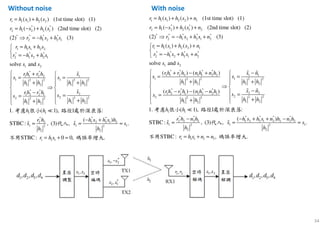
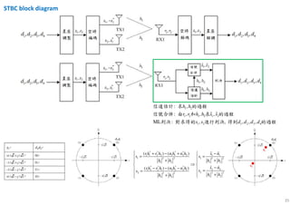
Space-Time Block Code
Space-Time Block Code (STBC)
• h1 and h2 are impulse
responses of two channels
whose envelopes follow
Rayleigh distribution
[ ]
*
1 2
1 2 *
2 1
x x
x x
x x
−
→
1 *
1 2x x = − x
2 *
2 1x x = x
1 2 * *
1 2 2 1 0x x x x⋅ − =< x x > =
( )
* * *
1 2 1 2
*
2 1 2 1
2 2
2 21 2
1 22 2
1 2
,
0
0
x x x x
x x x x
x x
x x
x x
−
= =
−
+
⋅ = = +
+
H
H
2
X X
X X I
where x1, x2 are modulated symbols
The received vectors are
1 1 1 2 2 1
* *
2 1 2 2 1 2
* * * *
2 1 2 2 1 2
1 1 2 1 1
* * * *
2 2 1 2 2
1 2 1
* *
2 1 2
( ) ( ) (1st time slot)
( ) ( ) (2nd time slot)
( ) ( )
. To solve we need to
y h x h x n
y h x h x n
y h x h x n
y h h x n
y h h x n
h h x
h h x
= + +
= − + +
= − + +
= + −
≡ −
H find the inverse of .H
( )
( )
( )
2 2*
1 21 21 2
* ** 2 2
2 12 1 1 2
2 2
1 2
2 2
1 2
1 1
*
2 2
1
1
1
0
0
digonal matrix inverse is
1
0
1
0
the estimate of the tramsmitted symbol is
H H
H
H
H H
H H H
H H
H H
h hh hh h
h hh h h h
h h
H H
h h
x y
x y
H
−+
−
−
+
= −− +
+
+
=
=
=
=
H
( )
( )
1 1
*
2 2
1 1
*
2 2
1
1
H H
H H
x n
H
x n
H H H
H H
n
x
H
x
n
−
−
= +
=
+
For a general m*n matrix the pseudo inverse is defined as
線代啟示錄 Moore-Penrose 偽逆矩陣](https://image.slidesharecdn.com/mimochannelcapacity-180509021101/85/MIMO-Channel-Capacity-33-320.jpg)


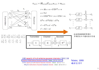
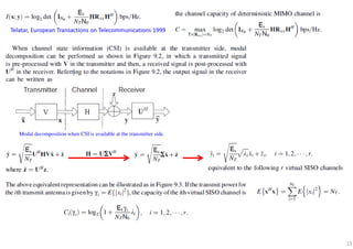
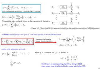
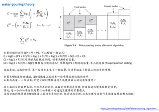
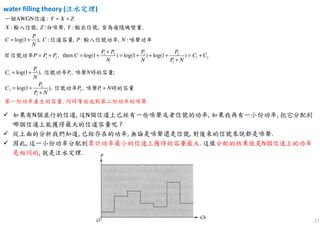
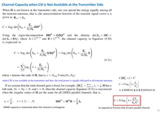
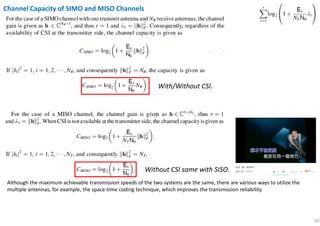
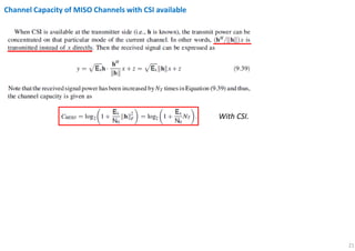
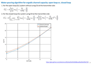
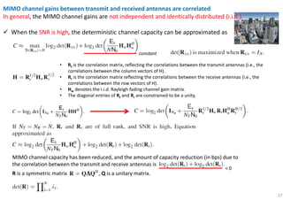
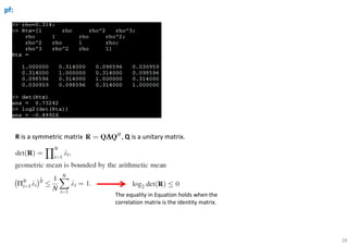
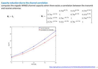
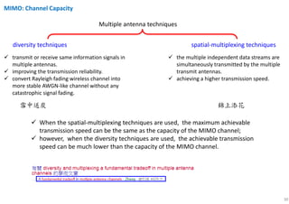
The document discusses the channel capacity of MIMO (Multiple Input Multiple Output) systems, focusing on various techniques such as spatial multiplexing and diversity techniques. It highlights the importance of channel state information (CSI) availability at the transmitter and outlines the capacity implications of different transmission strategies. Additionally, it explores the water-pouring algorithm and the concept of ergodic channel capacity in the context of random MIMO channels.


![[Year 2012-13] Mimo technology](https://cdn.slidesharecdn.com/ss_thumbnails/mimotechnology-180701101303-thumbnail.jpg?width=640&height=640&fit=bounds)