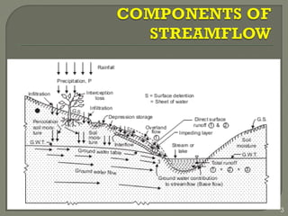
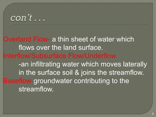
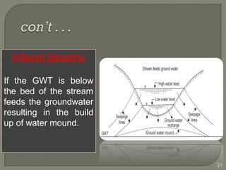
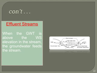
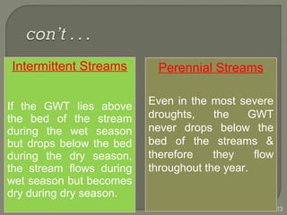
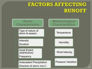
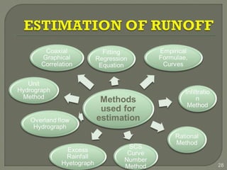
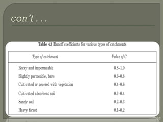
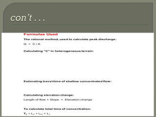
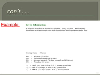
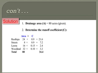
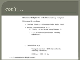
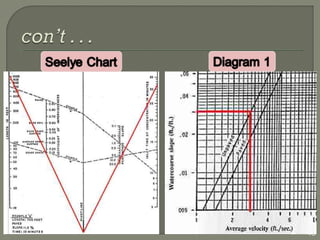
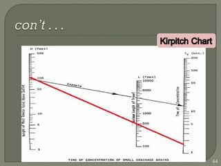
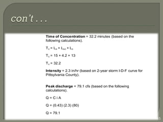
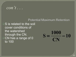
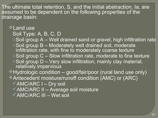
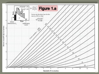
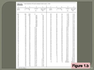
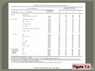
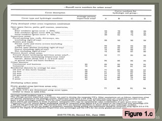
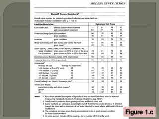
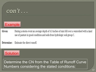
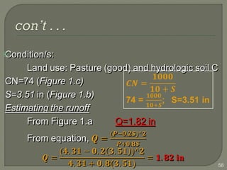
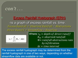
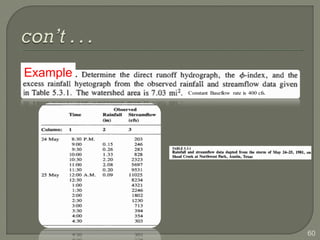
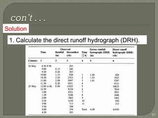
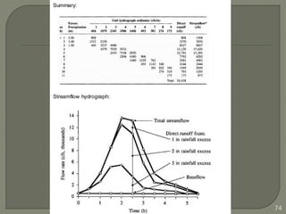
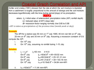
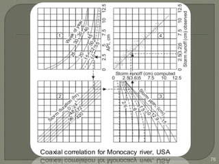
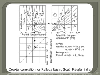
This document discusses various methods for estimating runoff from rainfall. It begins by defining components of stream flow such as overland flow, interflow, and baseflow. It then discusses catchment characteristics and methods for classifying streams. Various factors that affect runoff are identified, including drainage area, soil type, land use, and antecedent moisture conditions. Two primary methods for estimating runoff are presented: the Rational Method and the SCS Curve Number Method. Worked examples are provided to demonstrate how to apply both methods to calculate peak runoff rates from given rainfall and catchment property data.

2. A. COMPONENTS OF STREAM FLOW
B. CATCHMENT CHARACTERISTICS
C. MEAN AND MEDIAN ELEVATION
D. CLASSIFICATION OF STREAMS
E. ISOCHRONES
F. FACTORS AFFECTING RUNOFF
G. ESTIMATION OF RUNOFF
2

3. 3

4. Overland Flow- a thin sheet of water which
flows over the land surface.
Interflow/Subsurface Flow/Underflow
-an infiltrating water which moves laterally
in the surface soil & joins the streamflow.
Baseflow-groundwater contributing to the
streamflow.
4

5. Direct Runoff- general term used to include the
overland flow and interflow and snowmelt,
in some case.
Depression Storage- water stored in puddless,
pits, and small ponds.
Surface Detention/Detention Storage- value of
water in transit in overlandflow which has
not yet reached the stream channel.
5

6. Bank Storage- portion of runoff in a rising flood in
a stream, which is absorbed by permeable
boundaries of the stream above the normal
phreatic surface.
6

7. 7

8. 8

9. Drainage Basin- area of land drained by a river.
Catchment Area- area within the drainage
basin.
Watershed/Drainage Divide- edge of highland
surrounding a drainage basin & marks the
boundary b/w two drainage basins.
Source- beginning or start of a river.
Confluence- the point at w/c two rivers or stream
join.
9

10. Tributary- stream or small river w/c joins a larger
stream or river.
Mouth- the point where the river comes to the
end usually when entering a sea.
Concentration Point/Measuring Point- a single
point at w/c all surface drainage from a
basin comes together as outflow in the stream
channel.
10

11. 11
(Kirpich Equation)

12. Characteristics of Drainage Net
Number of Streams
Length of Streams
Stream Density
Drainage Density
12

13. 13

14. 14

15. Median Elevation- elevation at 50% area of the
catchment & is determined from the area-
elevation curve (hypsometric curve).
15
Hypsometric Curve

16. Example: The areas b/w different contour
elevations for the River A basin are given below.
Determine the mean and median elevation.
16

17. 17Computation of Mean Elevation of Basin

18. 18
Computation of Median Elevation of Basin

19. 19
Median Elevation for 50% of total area is read from
the curve as 350 m.

20. Streams may be classified as:
1.Influent Streams & Effluent Streams
2.Intermittent Streams & Perennial Streams
20

21. Influent Streams
If the GWT is below
the bed of the stream
feeds the groundwater
resulting in the build
up of water mound.
21

22. Effluent Streams
When the GWT is
above the WS
elevation in the stream,
the groundwater feeds
the stream.
22

23. Intermittent Streams
If the GWT lies above
the bed of the stream
during the wet season
but drops below the bed
during the dry season,
the stream flows during
wet season but becomes
dry during dry season.
23
Perennial Streams
Even in the most severe
droughts, the GWT
never drops below the
bed of the streams &
therefore they flow
throughout the year.
Perennial Streams
Even in the most severe
droughts, the GWT
never drops below the
bed of the streams &
therefore they flow
throughout the year.

24. Isochrones
These are time
contours and represent
lines of equal travel
time that are used to
show the time taken for
runoff water w/in a
drainage basin to reach
a lake, reservoir or
outlet.
24

25. 25

26. 26

27. 27

28. 28

29. 29

30. 30
Curve

31. 31

32. 32
r=1, correlation is perfect
giving a straight line plot
r=0, no relationships exist
b/w x & y
r 1, close linear
relationship

33. Example: Annual rainfall and runoff data for River M
for 17 years (1934-1950) are given below. Determine
the expected runoff for an annual rainfall 1050 mm.
33

34. 34
Year Rainfall (P) xRunoff ® y x^2 xy
1934.00 1088.00 274.00 1183744.00 298112.00 -211.82 -260.88 44869.21 68059.60 55261.02
1935.00 1113.00 320.00 1238769.00 356160.00 -186.82 -214.88 34903.03 46174.43 40145.08
1936.00 1512.00 543.00 2286144.00 821016.00 212.18 8.12 45018.85 65.90 1722.37
1937.00 1343.00 437.00 1803649.00 586891.00 43.18 -97.88 1864.21 9580.96 -4226.21
1938.00 1103.00 352.00 1216609.00 388256.00 -196.82 -182.88 38739.50 33445.96 35995.55
1939.00 1490.00 617.00 2220100.00 919330.00 190.18 82.12 36167.09 6743.31 15616.84
1940.00 1100.00 328.00 1210000.00 360800.00 -199.82 -206.88 39929.44 42800.31 41339.96
1941.00 1433.00 582.00 2053489.00 834006.00 133.18 47.12 17735.97 2220.07 6274.96
1942.00 1475.00 763.00 2175625.00 1125425.00 175.18 228.12 30686.80 52037.66 39960.84
1943.00 1380.00 558.00 1904400.00 770040.00 80.18 23.12 6428.27 534.43 1853.49
1944.00 1178.00 492.00 1387684.00 579576.00 -121.82 -42.88 14840.97 1838.90 5224.08
1945.00 1223.00 478.00 1495729.00 584594.00 -76.82 -56.88 5901.85 3235.60 4369.90
1946.00 1440.00 783.00 2073600.00 1127520.00 140.18 248.12 19649.44 61562.37 34780.26
1947.00 1165.00 551.00 1357225.00 641915.00 -134.82 16.12 18177.38 259.78 -2173.04
1948.00 1271.00 565.00 1615441.00 718115.00 -28.82 30.12 830.80 907.07 -868.10
1949.00 1443.00 720.00 2082249.00 1038960.00 143.18 185.12 20499.50 34268.54 26504.49
1950.00 1340.00 730.00 1795600.00 978200.00 40.18 195.12 1614.15 38070.90 7839.14
Sum 22097 9093 29100057 12128916
Mean 1299.823529 534.882353
Computation through Microsoft Excel
ο࢞ൌൌൌ࢞ൌൌ࢞ ο࢞ൌൌൌ࢞ൌൌ࢞ (ο࢞࢞^2 (ο࢞࢞^2 (ο࢞࢞࢞࢞ο࢞࢞

35. 35

36. 36

37. Rational Method
37
General Procedure
Step 1: Determine the drainage area (in acres.)
Step 2: Determine the runoff coefficient (C).
Step 3: Determine the hydraulic length or flow path that will be used to determine
the time of concentration.
Step 4: Determine the types of flow (or flow regimes) that occur along the flow path.
Step 5: Determine the time of concentration (Tc) for the drainage area.
Step 6: Use the time of concentration to determine the intensity.
Step 7: Input the drainage area, C value, and intensity into the formula to determine
the peak rate of runoff

38. 38

39. 39
Formulas Used
The rational method, used to calculate peak discharge:
Q = C i A
Calculating "C" in heterogeneous terrain:
Estimating travel time of shallow concentrated flow:
Calculating elevation change:
Length of flow × Slope = Elevation change
To calculate total time of concentration:
Tc = Lo + Lsc + Lc

40. Example:
40
Given Information
A project is to be built in southwest Campbell County, Virginia. The following
information was determined from field measurement and/or proposed design data:
Drainage Area: 80 acres
30% - Rooftops (24 acres)
10% - Streets and driveways (8 acres)
20% - Average lawns @ 5% slope on sandy soil (16 acres)
40% - Woodland (32 acres)
LO = 200 ft. (4% slope or 0.04 ft./ft.); average grass lawn.
LSC = 1000 ft. (4% slope or 0.04 ft./ft.); paved ditch.
LC = 2000 ft. (1% slope or 0.01 ft./ft.); stream channel.

41. 41
1. Drainage area (A) = 80 acres (given).
2. Determine the runoff coefficient(C):
Area × C
Rooftops 24 × 0.9 = 21.6
Streets 8 × 0.9 = 7.2
Lawns 16 × 0.15 = 2.4
Woodland 32 × 0.10 = 3.2
Total 80 34.4
SolutionSolution

42. 42
Determine the hydraulic path: This has already been given.
Determine flow regimes:
a. Overland flow (LO) = 15 minutes (using Seelye chart).
b. Shallow concentrated flow (LSC):
1. Velocity = 4 feet/second (using Diagram 1).
2. LSC = 4.2 minutes (based on the following
calculations).
c. Channel flow (LC):
Change in elevation = 20 feet (based on the
following calculations).
2000 feet × 0.01 = 20 feet
LC = 13 minutes (using Kirpitch chart).

43. 43

44. 44

45. 45
Time of Concentration = 32.2 minutes (based on the
following calculations).
Tc = Lo + Lsc + Lc
Tc = 15 + 4.2 + 13
Tc = 32.2
Intensity = 2.3 in/hr (based on 2-year storm I-D-F curve for
Pittsylvania County).
Peak discharge = 79.1 cfs (based on the following
calculations).
Q = C i A
Q = (0.43) (2.3) (80)
Q = 79.1

46. 46

47.  Soil Conservation Service(SCS) Curve Number
(CN) model estimates precipitation excess as a
function of cumulative precipitation, soil cover, land
use, and antecedent moisture
 SCS developed the method for small basins (< 400
sq. mi.) to "before" and "after" hydrologic response
from events.
47
SCS Curve Number Method

48. Where
Q = runoff (in)
P = rainfall (in)
S = potential maximum
retention after runoff
begins (in) and
Ia = initial abstraction (in) S)I(P
)I(P
Q
a
2
a
+−
−
=
48

49. Ia is all losses before
runoff begins it includes:
• water retained in
surface depressions,
• Water interception by
vegetation
• Evaporation and
infiltration.
Ia was found to follow:
Ia = 0.2*S
S)(P
S)(P
Q
2
*8.0
*2.0
+
−
=
49

50.  S is related to the soil
cover conditions of
the watershed
through the CN.
 CN has a range of 0
to 100
50
10
CN
1000
S −=
con’t . . .

51. The ultimate total retention, S, and the initial abstraction, Ia, are
assumed to be dependent on the following properties of the
drainage basin:
Land use
Soil Type: A, B, C, D
oSoil group A – Well drained sand or gravel, high infiltration rate
oSoil group B – Moderately well drained soil, moderate
infiltration rate, with fine to moderately coarse texture
oSoil group C – Slow infiltration rate, moderate to fine texture
oSoil group D – Very slow infiltration, mainly clay material,
relatively impervious
Hydrologic condition – good/fair/poor (rural land use only)
Antecedent moisture/runoff condition (AMC) or (ARC)
AMC/ARC I – Dry soil
AMC/ARC II – Average soil moisture
AMC/ARC III – Wet soil
51

52. 52

53. 53

54. 54

55. 55

56. 56

57. Example
Solution
Determine the CN from the Table of Runoff Curve
Numbers considering the stated conditions:
57

58. 58

59. 59
The excess rainfall hyetograph may be determined from the
rainfall hyetograph in one of two ways, depending on whether
streamflow data are available or not.

60. 60
Example

61. Solution
61
1. Calculate the direct runoff hydrograph (DRH).

62. 62
3. Estimate the rainfall abstraction rate.

63. 63
4. Calculate the excess rainfall hyetograph.

64. 64

65. Overland flow Method
65

66. 66

67. 67

68. Example
Solution
68

69. 69

70. 70

71. 71

72. 72

73. 73

74. 74

75. 75

76. 76

77. 77

78.  Engineering Hydrology by H.M. Raghunath
 Applied Hydrology by Ven Te Chow, et.al
 CE 374 K – Hydrology by Daene C. McKinney
 Rainfall-Runoff Modeling by Prof Ke-Sheng Cheng-
National Taiwan University
 Runoff Estimation by Dr. Ali Fares-NREM 600, Evaluation
of Natural Resources Management
 Runoff Estimation by Muhammad Khairudin bin Khalil
 Part 630 Hydrology Nationall Engineering
Handbook,USDA-NSCS
78

79. That’s all about RUNOFF.
79