This document discusses the quantization of electromagnetic radiation fields within the framework of quantum electrodynamics (QED). It begins by introducing the classical description of radiation fields in terms of vector potentials that satisfy the transversality condition. Next, it describes quantizing the classical radiation field by treating it as a collection of independent harmonic oscillators, with each oscillator characterized by a wave vector and polarization. Finally, it discusses how the quantization of these radiation oscillators leads to treating their canonical variables as non-commuting operators, in analogy to the quantization of position and momentum in non-relativistic quantum mechanics. This lays the foundation for a quantum description of radiation phenomena using the formalism of QED.

1. From First Principles January 2017 – R4.4
Maurice R. TREMBLAY
PART VII – QUANTUM ELECTRODYNAMICS
∫∫ +++++−=′ 65
2
56
2
)2,6()1,5()()6,4()5,3()()2,1;4,3( ττδγγ µµ ddKKsKKeiK bababa
ELECTRONS
VIRTUAL
QUANTUMTIME
1 2
3
4
5
6
)( 2
56s+δ
)6,4(+K
)1,5(+K
)2,6(+K
)5,3(+K
µγ
µγ
a b
Circa 1949
Chapter 2

2. Contents
PART VII–QUANTUM ELECTRODYNAMICS
Particles and Fields
Second Quantization
Yukawa Potential
Complex Scalar Field
Noether’s Theorem
Maxwell’s Equations
Classical Radiation Field
Quantization of Radiation Oscillators
Klein-Gordon Scalar Field
Charged Scalar Field
Propagator Theory
Dirac Spinor Field
Quantizing the Spinor Field
Weyl Neutrinos
Relativistic Quantum Mechanics
Quantizing the Maxwell Field
Cross Sections and the Scattering Matrix
Propagator Theory and Rutherford
2017
MRT
2
Scattering
Time Evolution Operator
Feynman’s Rules
The Compton Effect
Pair Annihilation
Møller Scattering
Bhabha Scattering
Bremsstrahlung
Radiative Corrections
Anomalous Magnetic Moment
Infrared Divergence
Lamb Shift
Overview of Renormalization in QED
Brief Review of Regularization in QED
Appendix I: Radiation Gauge
Appendix II: Path Integrals
Appendix III: Dirac Matrices
References

3. In order to study radiation phenomena in the quantum domain we shall first discuss in
detail the properties of the vector potential A satisfying the solenoïdal condition:
3
2017
MRT
0=• A∇∇∇∇
within the framework of classical electrodynamics. The equation above is known as the
transversality condition; it should not be confused with the Lorentz condition ∂µ Aµ =0.
The electric of magnetic fields derivable from vector potentials satisfying ∇∇∇∇•A=0 are
called transverse fields or radiation fields. Often the term transverse field or radiation
field is used to refer to a vector potential itself satisfying ∇∇∇∇•A=0.
Classical Radiation Field
The transversality condition ∇∇∇∇•A=0 is of interest under a variety of circumstances.
First, suppose Jµ =0. We can then consider a gauge transformation that eliminates the A0
component of Aµ and makes A obey ∇∇∇∇•A=0. Consider:
χ
χ
∇∇∇∇++++AAA =′→
∂
∂
−=′→ and
tc
AAA
1
000
such that:
0
1
A
tc
=
∂
∂χ
Since the A0 component of Aµ has been eliminated in the new gauge, the Lorentz
condition ∂µ Aµ =0 reduces to the transversality condition ∇∇∇∇•A=0.

4. Let us consider now the situation in which Jµ ≠0, as in the case of mutually interacting
electrons. We may first decompose A so that:
4
2017
MRT
||AAA ++++⊥=
where:
( ) ( )allongitudinandtransverse 0AA ==• ⊥ ||0 ××××∇∇∇∇∇∇∇∇
This can always be done. Here A⊥ and A| | are called respectively the transverse and the
longitudinal component of A.
Radiation)()(
2)()(
π4
)]([
2
1
H
ee
e
m
H
ji
ji
ji
j
j
j
j
j
+
−
+−= ∑∑ >
⊥
xx
xAp
where HRadiation is the free field Hamiltonian of A⊥ only. Note that nowhere in this equation
do A0 and A| | appear explicitly.
In 1930, E. Fermi was able to show that A| | and A0 together give rise to the
instantaneous static Coulomb interaction between the charged particles, whereas A⊥
accounts for the electromagnetic radiation of moving charged particles. The total
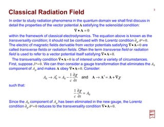
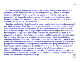
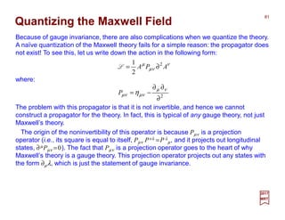
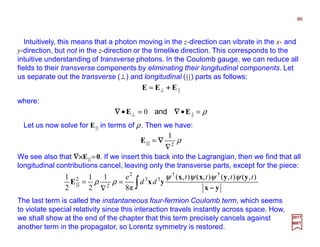
Hamiltonian of the charged particles (treated nonrelativistically) and the electromagnetic
fields generated by them can be written (apart from the magnetic moment interaction) as
(c.f., Appendix I: Radiation Gauge):

5. Fermi's formalism based on the Hamiltonian H=HEM +HRadiation above is called the
radiation (or Coulomb) gauge method. Since this decomposition shown in the
Hamiltonian is not relativistically covariant, nor is the transversality condition itself, the
whole formalism appears noncovariant; each time we perform a Lorentz transformation,
we must simultaneously make a gauge transformation to obtain a new set of A and A0.
5
2017
MRT
tc ∂
∂
−==
A
EAB
1
and××××∇∇∇∇
It is worth studying a theory of transverse electromagnetic field before we learn about
more sophisticated formalisms. When the theory is quantized, it provides simple and
physically transparent descriptions of a variety of processes in which real photons are
emitted, absorbed, or scattered. The three basic equations we work with for the free-field
case are:
as well as:
0
1
2
2
2
2
=
∂
∂
−∇
tc
A
A
where A satisfies the transversality condition ∇∇∇∇•A=0. Note that for the time being we
will include the velocity of light constant c in the equations – for old time sake! This will
especially come to bear when we introduce the angular momentum ω=|k|c in the
equations that will follow.

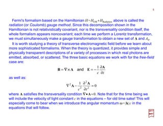
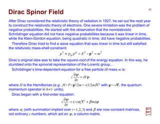
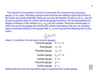
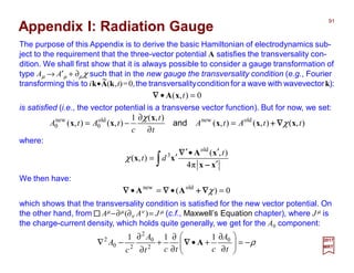
6. At a given instant, say starting at t =0, we expand the vector potential A in terms of
Fourier series and assume periodic boundary conditions for A enclosed in a box taken to
be a cube of volume V and of side L=V 1/3. Remembering the reality of A, we have:
6
2017
MRT
∑ ∑=
=
+=
k
kkkk xuxuxA
2,1
**
0
])()0()()0([
1
),(
r
rrrrt
cc
V
t
(N.B., ckr (0) and its complex conjugate c*
kr(0) are Fourier coefficients) where:
xk
k εxu •
= ir
r e)( )(
and εεεε(r), called a (linear) polarization vector, is a real unit vector whose direction
depends on the propagation direction k (i.e., the wave vector). Given k, we choose εεεε(1)
and εεεε(2) in such a way that {εεεε(1),εεεε(2),k/|k|} for a right-handed set of mutually orthogonal
unit vectors (N.B., εεεε(1) and εεεε(2) are, in general, not along the x- and the y-axes since k is,
in general, not along the z-axis). Since εεεε(r) is perpendicular to k, the transversality
condition is guaranteed. The Fourier components ukr satisfy:
sr
sr
sr
srsr d
V
d
V
δδδδ kk
kk
kk
kkkk
uu
uu
xuux ′−
′
′
′′ =








•
•
=• ∫∫ ,**
3*3 11
and
where:
because of the periodic boundary conditions.
( )K,2,1
π2
,, ±±== n
L
n
kkk zyx

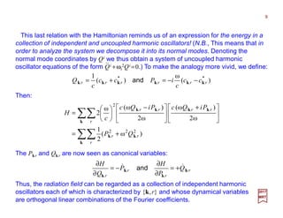
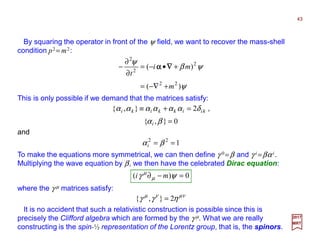
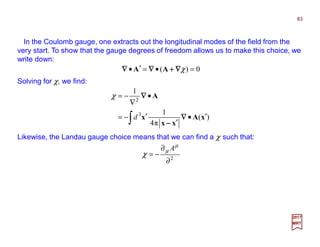
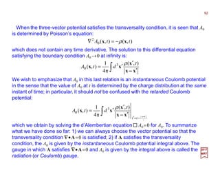
7. To obtain A(x,t) for t≠0, we simply replace ckr (0) and c*
kr (0) by:
7
2017
MRT
ti
rr
ti
rr ctcctc ω**ω
e)0()(e)0()( kkkk == −
and
where the angular frequency is given by:
ck=ω
With this replacement, both the wave equation ∇2A−(1/c2)∂2A/∂t2 =0 and the reality
condition on A are satisfied. So:
∑∑
∑∑
∑∑
⋅−⋅
+•−−•
•−•
+=
+=
+=
k
kk
k
xk
k
xk
k
k
xk
k
xk
k
εε
εε
εεxA
r
xkir
r
xkir
r
r
tiir
r
tiir
r
r
ir
r
ir
r
cc
V
cc
V
tctc
V
t
]e)0(e)0([
1
]e)0(e)0([
1
]e)(e)([
1
),(
)(*)(
ω)(*ω)(
)(*)(
where:
tctxkxk kxkxk −•=−•=≡⋅ ωµ
µ
since:
],[]ω,[ xk txk == µµ
and

8. The Hamiltonian of the field is:
8
2017
MRT
A typical term we must evaluate for the |B|2 integration is:
∫∫ 







∂
∂
+=−=
2
23223 1
2
1
)(
2
1
tc
ddH
A
AxEBx ××××∇∇∇∇
sr
sr
srsrsr
V
c
d
ddd
δδ kk
kk
kkkkkk
uux
uuxuuxuux
′
′
′′′






=
•∇−=
•+•=•
∫
∫∫∫
2
*23
*3*3*3
ω
)]([)]([)()( ××××∇∇∇∇××××∇∇∇∇××××∇∇∇∇××××∇∇∇∇××××∇∇∇∇
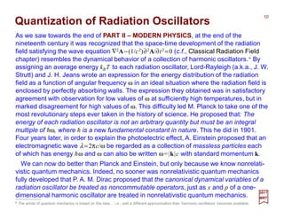
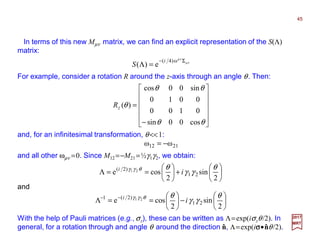
where we have used the periodic boundary conditions and the identity ∇∇∇∇××××(∇∇∇∇××××X)=∇∇∇∇(∇∇∇∇•X)
−−−−∇2X. Similarly, for the |E|2 integration it is useful to evaluate first:
*
2
**3 ω
)(
1
)(
1
srsrssrr ccV
c
c
tc
c
tc
d kkkkkkkk uux ′′′′ 





=





∂
∂
•





∂
∂
∫ δδ
Using these relations, we obtain:
∑∑ 





=
k
kk
r
rrcc
c
H *
2
ω
2
where ckr is a time-independent Fourier coefficient satisfying ckr =−ω2ckr.−

9. This last relation with the Hamiltonian reminds us of an expression for the energy in a
collection of independent and uncoupled harmonic oscillators! (N.B., This means that in
order to analyze the system we decompose it into its normal modes. Denoting the
normal mode coordinates by Qi we thus obtain a system of uncoupled harmonic
oscillator equations of the form Qi +ωi
2Qi =0.) To make the analogy more vivid, we define:
9
2017
MRT
)(
ω
)(
1 **
rrrrrr cc
c
iPcc
c
Q kkkkkk −−=+= and
Then:
∑∑
∑∑
+=





 +





 −






=
k
kk
k
kkkk
r
rr
r
rrrr
QP
PiQcPiQc
c
H
)ω(
2
1
ω2
)ω(
ω2
)ω(ω
2
222
2
The Pkr and Qkr are now seen as canonical variables:
r
r
r
r
Q
P
H
P
Q
H
k
k
k
k
&& +=
∂
∂
−=
∂
∂
and
Thus, the radiation field can be regarded as a collection of independent harmonic
oscillators each of which is characterized by {k,r} and whose dynamical variables
are orthogonal linear combinations of the Fourier coefficients.
⋅⋅

10. As we saw towards the end of PART II – MODERN PHYSICS, at the end of the
nineteenth century it was recognized that the space-time development of the radiation
field satisfying the wave equation ∇2A−(1/c2)∂2A/∂t2 =0 (c.f., Classical Radiation Field
chapter) resembles the dynamical behavior of a collection of harmonic oscillators.* By
assigning an average energy kBT to each radiation oscillator, Lord-Rayleigh (a.k.a., J. W.
Strutt) and J. H. Jeans wrote an expression for the energy distribution of the radiation
field as a function of angular frequency ω in an ideal situation where the radiation field is
enclosed by perfectly absorbing walls. The expression they obtained was in satisfactory
agreement with observation for low values of ω at sufficiently high temperatures, but in
marked disagreement for high values of ω. This difficulty led M. Planck to take one of the
most revolutionary steps ever taken in the history of science. He proposed that: The
energy of each radiation oscillator is not an arbitrary quantity but must be an integral
multiple of hω, where h is a new fundamental constant in nature. This he did in 1901.
Four years later, in order to explain the photoelectric effect, A. Einstein proposed that an
electromagnetic wave λ=2πc/ω be regarded as a collection of massless particles each
of which has energy hω and ω can also be written ω=|k|c with standard momentum k.
10
2017
MRT
We can now do better than Planck and Einstein, but only because we know nonrelati-
vistic quantum mechanics. Indeed, no sooner was nonrelativistic quantum mechanics
fully developed that P. A. M. Dirac proposed that the canonical dynamical variables of a
radiation oscillator be treated as noncommutable operators, just as x and p of a one-
dimensional harmonic oscillator are treated in nonrelativistic quantum mechanics.
Quantization of Radiation Oscillators
* The whole of quantum mechanics is based on this idea… i.e., until a different approximation than ‘harmonic oscillators’ becomes available.

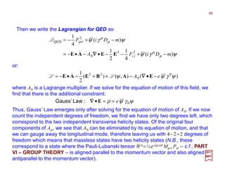
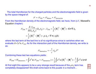
11. We postulate that P and Q of the radiation oscillators are no longer mere numbers but
are operators satisfying:
11
2017
MRT
0],[0],[],[ === ′′′′ srsrsrsr PPQQiPQ kkkkkkkk and,δδh
We next consider linear combinations of Pkr and Qkr given by:
)ω(
ω2
1
)ω(
ω2
1 †
rrrrrr PiQaPiQa kkkkkk −=+=
hh
and
The akr and a†
kr are seen to be the operator analogs of the Fourier coefficients ckr and
c†
kr when we insert a factor to make akr and a†
kr dimensionless:
rr acc kk
ω2
h
→
They satisfy the commutation relations:
srsrsrsr QP
i
PQ
i
aa δδ kkkkkkkk ′′′′ =+−= ],[
2
],[
2
],[ †
hh
0],[],[ ††
== ′′ srsr aaaa kkkk
and
These commutation relations are to be evaluated for operators taken at equal times
(e.g., [akr,a†
k′s] actually stands for [akr(t),a†
k′s(t)] in the Heisenberg Picture where
operators incorporate a dependency on time, but the state vectors are time-
independent).

12. Before we begin the physical interpretations of akr and a†
kr, it is instructive to study the
properties of the operator defined by:
12
2017
MRT
We have:
rrr aaN kkk
†
=
rsr
rssssr
rssssrsr
a
aaaaaa
aaaaaaNa
kkk
kkkkkk
kkkkkkkk
δδ ′
′′′′
′′′′′
=
−=
−=
],[],[
],[
††
††
Similarly:
††
],[ rsrsr aNa kkkkk δδ ′′ −=
For the time being, we will suppress the indices k and r.

13. Unlike a and a†, the operator N is Hermitian. The Hermiticity of N encourages us to
consider a normalized eigenvector of the operator N denoted by |n〉 such that:
13
2017
MRT
nnnN =
where n is the eigenvalue of N. Because N is Hermitian, n must be real. Now:
nannaNanaN ††††
)1()( +=+=
where we have used [a†,N]=−a† above. This can be viewed as a new eigenvalue
equation in which the eigenvalue a†|n〉 is shown to have eigenvalue n+1. Similarly:
nannaN )1( −=
The roles of a† and a are now clear; a† (a) acting on |n〉 gives a new eigenvector with
eigenvalue increased (decreased) by one. So:
11†
−=+= −+ ncnancna and
where c+ and c− are constants. To determine c± we evaluate:
1],[11 ††††22
+=+===++= ++ nnaaNnnaannananncc
and
The phases of c± are indeterminate; they may be chosen to be zero at t=0 by
convention.
nnaannanac ===−
†2

14. We thus have, at t=0:
14
2017
MRT
Meanwhile:
111†
−=++= nnnannna and
0†
≥== naannNnn
since the norm of a|n〉 must be positive. This immediately tells us that n cannot be a
noninteger; otherwise, the eigenvalue of |n〉 could be made to decrease indefinitely as
we successfully apply a, and n would eventually take negative values, in contradiction to
n≥0 above. On the other hand, if n is a positive integer, successive applications of the
operator a proceed as:
000211221 ===−= aaannna ,,,L
Note that we obtain a null vector 0 (to be distinguished from |0〉) when a is applied to |0〉.
By applying a to such a null vector, we again obtain a null vector. Hence n=0 is the
lowest possible eigenvalue of the operator N.

15. Explicit matrix representations of a, a†, and N consistent with the commutation relations
[a,a†]=1 & [a,a]=[a†,a†]=0, [a,N]=a and [a†,N]=−a† above* can be written as follows:
15
2017
MRT
















=
















=
OMMMMM
L
L
L
L
OMMMMM
L
L
L
L
00300
00020
00001
00000
40000
03000
00200
00010
†
aa &
and
















=
OMMMM
L
L
L
L
3000
0200
0010
0000
N
* Technically, these were written above in the form:
†††††
],[],[0],[],[],[ rsrsrrsrsrsrsrsrsr aNaaNaaaaaaa kkkkkkkkkkkkkkkkkk δδδδδδ ′′′′′′′′ −===== and,&

16. They are assumed to act on a column vector represented by:
16
2017
MRT
where only the (n+1)-entry is different than zero and where the superscript T means
‘transpose’ (i.e., a transposed matrix is a new matrix whose rows are the columns of the
original).
[ ]T
LL
M
M
01000
0
1
0
0
0
≡






















=n

17. The algebra developed so far can be applied to a physical situation in which the
number of photons with given momentum and polarization is increased or decreased.
The wave vector k is identified with the photon momentum p divided by h, and r
represents the polarization state of the photon. We interpret an eigenvector of Nkr as the
state vector for a state with a definite number of photons in state (k,r). To represent a
situation in which there are many types of photons with different sets of (k,r), we
consider the direct product of eigenvectors as follows:
17
2017
MRT
LLKK iiii rrrrrr nnnnnn kkkkkk 22112211
,,,, =
This state vector corresponds to the physical situation in which there are Nk1r1
photons
present in state (k1,r1), Nk2r2
photons present in state (k2,r2), &c. The number nkr is the
occupation number for state (k,r).

18. As an example, the state represented by:
18
2017
MRT
since the eigenvalue of Nkr is one (c.f., Nkra†
kr |n〉=(n+1)a†
kr |n〉 above). A two-photon
state is represented by the normalized eigenvector:
LL ii rrr kkk 0000 2211
=
has the property that if akr is applied to it, then we obtain a null vector for any (k,r).
Hence the eigenvalue of Nkr =a†
kr akr is zero for any (k,r). Therefore the state
corresponding to |0〉 above is called the vacuum state. A single-photon state with definite
(k,r) is represented by:
0†
rak
0
2
1 ††
rr aa kk
when the two photons are in the same state, and:
0††
rr aa kk
when the two photons are in different states. More generally:
0)(
1
,, †
2211 ∏=
ii
iri
ii
iir
n
r
r
rr a
n
nn
k
k
k
kk
k
K

19. Note that when a†
ki ri
is applied to the most general state vector, we obtain:
19
2017
MRT
Thus a†
ki ri
has the property of creating an additional photon in state (ki,ri), leaving the
occupation numbers of states other than (ki,ri) unchanged. For this reason a†
kr is called
the creation operator for a photon in state (k,r). Similarly, akr can be interpreted as the
annihilation operator for a photon in state (k,r). In contrast, Nkr, being diagonal, does not
change the occupation number of photons; it simply gives as its eigenvalue the number
of photons in state (k,r).
KKKK ,1,,,1,,,, 22112211
†
++= iiiiiiii
rrrrrrrr nnnnnnna kkkkkkkk
Our formalism is capable of describing a physical situation in which the number of
photons in a given state is unrestricted. Moreover, any many-photon systems we can
construct is necessarily symmetric under interchange of any pair of labels. For instance,
the two-photon state a†
kr a†
kr |0〉 above is evidently symmetric under interchange (k,r)↔
(k′,s) since:
The quantization of the radiation field is shown, although using a somewhat
different notation, in the Appendix of PART V – THE HYDROGEN ATOM.
00 ††††
ssrr aaaa kkkk ′′=
because of the commutation rule. Thus, the state vectors we obtain by applying creation
operators to |0〉 are automatically consistent with Bose-Einstein statistics. With
essentially no modifications our formalism can be applied to physical states made up of
identical particle other than photons as long as they obey Bose-Einstein statistics.

20. Let us begin our discussion by quantizing the simplest possible relativistic field theory,
the free scalar field. The theory was proposed in various papers by six different
physicists in 1926-27: W. Gordon, O. Klein, V. Fock, E. Schrödinger, Th. de Donder & H.
van den Dungen, and J. Kudar. The Lagrangian (density) is given by:
20
2017
MRT
Klein-Gordon Scalar Field
Historically, the quantization of the Klein-Gordon equation caused much confusion.
Schrodinger,even before he postulated his celebrated nonrelativistic equation,i∂Ψ(x,t)/∂t
=HΨ(x,t), considered this relativistic equation but ultimately discarded it because of
problems with negative probabilities and negative energy states. In any fully relativistic
equation, we must obey the mass-shell condition pµ
2= E2 −p2 =m2. This means that the
energy is given by:
22
2
1
2
1
φφφ µ
µ m−∂∂=L
22
mE +±= p
The energy can be negative, which is quite disturbing. Even if we banish the negative
energy states by fiat, we find that interactions with other particles will reduce the energy
and create negative energy states. This means that all positive energy states will
eventually collapse into negative energy states, destabilizing the entire theory! However,
the solution of these problems with negative probability and negative energy can be
resolved once one quantizes the theory…
where φ =φ(x,t). From this Lagrangian we get the equation of motion (∂2/∂t2 −∇2 +m2)φ(x,t)
=0 (or (∂µ∂µ +m2)φ(x)=0) which is the well-known Klein-Gordon (wave) equation.

21. The canonical quantization program begins with fields φ and their conjugate momen-
tum fields π, which satisfy equal time commutation relations among themselves.Then the
time evolution of these quantized fields is governed by a HamiltonianH=∫d3x H. Thus,
we closely mimic the dynamics found in ordinary quantum mechanics. We begin by sin-
gling out time as a spatial coordinate and then defining the canonical conjugate field to φ:
We first introduce the Hamiltonian (density) as:
),(
),(
),( t
t
t x
x
x φ
φδ
δ
π &
&
==
L
21
2017
MRT
])([
2
1 2222
φφπφπ m++=−= ∇∇∇∇LH &
Then the transition from classical mechanics to quantum field theory begins when we
postulate the commutation relations between the field and its conjugate momentum:
)()],(,),([ 3
yxyx −−−−δπφ itt =
with the right-hand side proportional to h which we set to unity. Also, [φ,φ]=[π ,π]=0.
Much of what follows is a direct consequence of this commutation relation above.
There are an infinite number of ways in which to satisfy this relationship, but our strategy
will be to find a specific Fourier representation of this commutation relation in terms of
plane waves. When these plane-wave solutions are quantized in terms of harmonic
oscillators, we will be able to construct the multiparticle Hilbert space and also find a
specific operator representation of the Lorentz group in terms of oscillators.

22. We first define the quantity:
We want a decomposition of the scalar field where the energy k0 =E is positive, and
where the Klein-Gordon equation is explicitly obeyed. In momentum space, the operator
∂µ
2 +m2 (c.f., (∂µ∂µ +m2)φ (x)=0 above) becomes k2 −m2. Therefore, we choose:
xp•−=≡⋅ tExkxk µ
µ
22
2017
MRT
∫
⋅⋅−
+−= ]e)(e)()[()(
)π2(
1
)( †
0
224
23
xkixki
kAkAkmkkdx θδφ
where θ is a step function (i.e., θ(k0)=+1 if k0 >0 and θ(k0)=0 otherwise), and where A(k)
are operator-valued Fourier coefficients. It is now obvious that this field satisfies the
Klein-Gorgon equation (i.e., if we hit this expression with (∂µ
2+m2), then this pulls down a
factor of k2 −m2, which then cancels against the delta function δ (k2 −m2)).
We can simplify this expression by integrating out dk0 (which also breaks manifest
Lorentz invariance). To perform the integration, we need to re-express the delta function.
We note that a function f (x), which satisfies f (a)=0, obeys the relation:
)(
)(
)]([
af
ax
xf
′
−
=
δ
δ
for x near a. Since k2 =m2 has two roots, we find:
0
220
0
220
22
2
)(
2
)(
)(
k
mk
k
mk
mk
++
+
+−
=−
kk δδ
δ

23. Putting this back into the integral, and using only the positive value of k0, we find:
23
2017
MRT
∫∫ ∫∫ ∫∫ =−=+−=−
∞
k
k
k
kkk
ω2
)ω(
2
1
)(
2
1
)()(
3
0
00
0322
00
03
0
224 d
k
k
kddmk
k
kddkmkkd δδθδ
where ωk ≡√(k2 +m2) and d4k ≡d3kdk0. Now let us insert this expression back into the
Fourier decomposition of φ(x). We now find:
∫∫ +=+= ⋅⋅−
)]()()()([]e)(e)([
ω2)π2(
1
)( *†3†
3
23
xekaxekadkaka
d
x kk
xkixki
k
k
k
φ
with a(k) ≡ A(k)/√(2ωk). Furthermore:
where:
∫ +−== )]()()()([ω)()( *†3
xekaxekadixx kkkkφπ &
kω2
e
)π2(
1
)( 23
xki
k xe
⋅−
=
and note that with the k0 appearing in k⋅x it is now equal to ωk. We can also invert these
relations, solving for the Fourier modes a(k) in terms of the original scalar field:
with the operator:
∫∫ ∂=∂= )()()()()()( 0
3†
0
*3
xxedikaxxedika kk φφ
tt
xx and
BABABA )(∂−∂≡∂
t
+ −

24. Because the fields satisfy equal-time canonical commutation relations, the Fourier
modes must also satisfy commutation relations:
24
)()](,)([ 3†
kk ′=′ −−−−δkaka
and all other commutators (i.e., between a† and itself and a and itself) are zero.
Now we can calculate the Hamiltonian H in terms of these Fourier modes using the
Hamiltonian density H =½[π2 +(∇∇∇∇φ)2 +m2φ2] introduced above with ∇∇∇∇φ ≡∂iφ :
∫
∫
∫∫






+=
+=
+∂∂+==
)()(ω
)]()()()([ω
2
1
][
2
1
†3
††3
22233
kakad
kakakakad
mddH ii
k
k
k
k
xx φφφπH
Similarly, we can calculate the momentum:
∫
∫∫






+=
+=−=
)()(
)]()()()([
2
1
†3
††33
kakad
kakakakadd
kk
kkxP φπ ∇∇∇∇
2017
MRT
1
‒
2
+
1
‒
2
+
(N.B.,Both H and P are divergent because of the ½ factor appearing in the infinite sum).

25. With these expressions, the operators Pµ and Mµν generate translations and Lorentz
rotations:
as they should. If we exponiate these generators of translation and Lorentz rotations, we
can calculate how the field φ(x) transforms under the Poincaré group. Let us define:
φφφφ µννµµν
µµ )(],[],[ ∂−∂=∂= xxMiPi and
25
2017
MRT
µ
µ
µν
µν PaiMi
aU
−−
=Λ
ω
2
1
e),(
where Λµν =ηµν +ωµν +…. Then it can be shown that:
)(),()(),( 1
axaUxaU +Λ=ΛΛ −
φφ
This demonstrates that φ(x) transforms as a scalar field under the Poincaré group.
Now that we have successfully shown how to quantize the Klein-Gordon field, we must
now calculate the eigenstates of the Hamiltonian to find the spectrum of states. Let us
define the vacuum states as follows:
00)( =ka
By convention, we call a(k) an annihilation operator. We define a one-particle state via
the creation operator a†(k) as a Fock space (i.e., an algebraic construction used in
quantum mechanics to construct the quantum states space of a variable or unknown
number of identical particles from a single particle Hilbert space HHHH ):
kka =0)(†

26. The problem with this construction, however, is that the energy associated with the
vacuum state is formally infinite because of the presence of ½ in the sum in the equation
H=∫d3k ωk[a†(k)a(k)+½]=∫d3k ωka†(k)a(k) +½∫d3k ωk above. We will drop this infinite term,
since infinite shifts in the Hamiltonian cannot be measured. Dropping the zero point
energy in the expression for harmonic oscillators has a simple counterpart in x space.
The zero-point energy emerged when we commuted creation and annihilation operators
past each other. Dropping the zero-point energy is therefore equivalent to moving all
creation operators to the left and annihilation operators to the right. This operation, in x
space, can be accomplished by normal ordering. Since the product of two or more fields
at the same point is formally divergent (i.e., limx→y φ(x)φ(y)=∞), we can remove this
divergence by the normal ordering operation, which corresponds to moving the part
containing the creation operators to the left and the annihilation operators to the right.
For example, if we decompose φ(x)=φ†(x)+φ∅(x), where †(∅) represent the creation
(annihilation) part of an operator with negative (positive) frequency, then we define:
Then, by applying the normal ordering to the definition of the Hamiltonian, we can simply
drop the ½ appearing in H above. From now on, we assume that when two fields are
multiplied at the same point in space-time, they are automatically normal ordered.
26
2017
MRT
Once we have normal ordered the operators, we now have an explicitly positive
Hamiltonian. In this fashion, we have been able to handle the question of negative
energy states for the Klein-Gordon theory.
)()()()()()()()(:)()(: yxxyyxyxyx φφφφφφφφφφ +++≡ † † † †∅ ∅ ∅ ∅

27. One essential point in introducing these creation and annihilation operators is that we
can write down the N-particle Fock space:
This is the chief distinguishing feature between first and second quantization. In first
quantization, we quantized the xi corresponding to a single particle. First quantized
systems were hence inherently based on single-particle dynamics. In the second
quantized formalism, by contrast, we quantize multiparticle states. To count how many
particles we have of a certain momentum, we introduce the number operator:
∫= )()(†3
kakadN k
27
2017
MRT
0)()()(,,, †
2
†
1
†
21 NN kakakakkk LK =
The advantage of this number operator is that we can now calculate how many particles
there are of a certain momentum.

28. Forexample,let |n(k)〉 equal a state consistentof n(k) identical particles with momentumk:
Then the number operator N acting on this multiparticle state just counts the number of
particles present:
28
2017
MRT
0)]([
!)(
1
)( )(† kn
ka
kn
kn =
By commuting a(k) to the right, until they annihilate on the vacuum, we see that:
)()()( knknknN =
that is, N simply counts the number of state there are at momentum k. Not surprisingly, a
multiparticle state, consisting of many particles of different momenta, can be
represented as a Fock space:
0)]([
!)(
1
)()()(
1
)(†
21 ∏=
=
m
i
kn
i
i
m
i
ka
kn
knknkn L
)()()()()()()( 21
1
21 m
m
i
im knknknknknknknN LL








= ∑=
Finally, it is essential to notice that the norm of these multiparticle states is positive.
If we define 〈k |≡〈0 |a(k) and set 〈0|0〉=1, then the norm is given by 〈k|k〉=+δ 3(k−−−−k′).
The norm is positive because the appropriate sign appears in the above commutation
relation [a(k),a†(k)]=δ 3(k−−−−k′).

29. We can generalize our discussion of the Klein-Gordon field by postulating the existence
of several scalar fields. In particular, we can arrange two independent scalar field into a
single complex field:
The action then becomes:
)(
2
1
21 φφφ +=
29
2017
MRT
Charged Scalar Field
φφφφ µ
µ
†2†
m−∂∂=L
Nevertheless, if we insert this decomposition of φ into the action S, then we find the sum
of two independent actions for φ1 and φ2, since it is the case for the Lagrangian (density).
The quantization of this action proceed as before by calculating the conjugate field and
postulating the canonical commutation relations. The conjugate field is given by:
†
φ
φδ
δ
π &
&
==
L
The commutation relations now read:
)()],(,),([ 3
yxyx −−−−δπφ itt =
which will be a habitual rough-in coinage of the term since the action is actually given by:
∫= LxdS 4

30. Since the decomposition of the scalar field (c.f., Klein-Gordon Scalar Field chapter) was:
where i=1,2. Then the canonical commutation can be satisfied if the Fourier compo-
nents obey the following commutation relations:
30
2017
MRT
∫
⋅⋅−
+= ]e)(e)([
ω2)π2(
1
)( †
3
23
xki
i
xki
ii kaka
d
x
k
k
φ
jiji kaka δδ )()](,)([ 3†
kk ′=′ −−−−
All other commutators vanish. Similarly, we can choose the decomposition:
)]()([
2
1
)()]()([
2
1
)( †
2
†
1
†
21 kaikakakaikaka −=+= and
as well as:
)]()([
2
1
)()]()([
2
1
)( †
2
†
1
†
21 kaikakbkaikakb +=−= and
For these operators, the new commutation relations read:
)()](,)([)](,)([ 3††
kk ′=′=′ −−−−δkbkbkaka
All other commutators are zero.
∫
⋅⋅−
+= ]e)(e)([
ω2)π2(
1
)( †
3
23
xkixki
kaka
d
x
k
k
φ
we can always decompose the φ = (1/√2)(φ1 +φ2) field in terms of the Fourier components:

31. Now let us construct the symmetries of the action and the corresponding Noether
currents. The action is symmetric under the following transformation:
which generates a U(1) symmetry. Written out in components, we find the following
SO(2) transformation (c.f., PART VI – GROUP THEORY):
††
ee φφφφ θθ ii −
→→ and
31
2017
MRT











 −
=





′
′
2
1
2
1
cossin
sincos
φ
φ
θθ
θθ
φ
φ
This symmetry generates a Noether current (e.g., Jµ =(δ L/δ ∂µφ)(δφ/δθ)) which equals:
φφφφ µµµ
††
∂−∂= iiJ
Now let us calculate the charge Q corresponding to this current in terms of the quantized
operators:
ba NNkbkbkakadidQ −=−=−= ∫∫ )]()()()([)( ††3††3
xx φφφφ &&
where the number operator for the a and b oscillators is given by:
∫∫ == )()()()( †3†3
kbkbdNkakadN ba xx and
Historically, this conserved current caused a certain amount of confusion. If J 0 is
considered to be the probability density of the wave function, then it can be negative,
and hence negative probabilities creep into the theory.

32. In 1934, W. Pauli and V. Weisskopf finally gave the correct quantum interpretation of
these negative probabilities:
Second, we will interpret the b† oscillators as the creation operator for a new state of
matter, antimatter. It was Dirac who originally grappled with these new states found in
any relativistic theory and deduced the fact that a new form of matter, with opposite
charge, must be given serious physical consideration. The discovery of the antielectron
(i.e., the positron) gave graphic experimental proof of this conjecture.
32
2017
MRT
First, because of the crucial minus sign appearing in front of the b oscillators, we will
find it convenient to redefine the current Jµ as the current corresponding to the electric
charge, rather than probability density, so that the a oscillators correspond to a positively
charged particle and the b oscillators correspond to a negatively charged one. In this
way, we can construct the quantum theory of charged scalar particles, where the minus
sign appearing in the current is a desirable feature, rather than a fatal illness of the
theory.
Third, we no longer have a simple, single-particle interpretation of the φ(x), which now
contains both matter and antimatter fields. Thus, we must abandon the strict single-
particle interpretation for φ and reinterpret it as a field.

33. Now that we have defined the canonical commutation relations among the particle fields,
we are interested in how these particles actually move in space-time.
To solve this equation, we use the standard theory of Green functions. We first define a
propagator that satisfies:
33
2017
MRT
Propagator Theory
)()()( 22
xJxm =−∂ φµ
)()()( 422
yxyxm F −−=−∆−∂ δµ
Then the solution of the interacting φ field is given by:
∫ −∆−= )()()()( 4
0 yJyxxdxx Fφφ
where φ0(x) is any function that satisfies the Klein-Gordon equation without any source
term (i.e., (∂µ∂µ +m2)φ0(x)=0). If we hit both sides of this expression with (∂µ
2 +m2), then
we find that it satisfies the original Klein-Gordon equation in the presence of a source
term.
To define a propagator, and also anticipate interactions, let us modify the Klein-Gordon
equation to include a source term J(x):

34. The way to solve this last equation is to take the Fourier transform:
If we hit both sides of this equation with (∂µ
2 +m2), then we can solve for ∆F(k):
34
2017
MRT
∫ ∆=−∆ −⋅−
)(e
)π2(
)( )(
4
4
k
xd
yx F
yxki
F
22
1
)(
mk
kF
−
=∆
At this point, however, we realize that there is an ambiguity in this equation. The integral
over d4k cannot be performed on the real axis, because the denominator diverges at kµ
2
=m2. This same ambiguity occurs even in the classical theory of wave equations, and is
not specific to the Lorentz covariant theory. The origin of this ambiguity lies not in the
mathematics, but in the physics, in the fact that we have yet to fix our boundary
conditions.

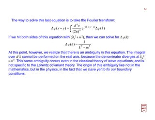
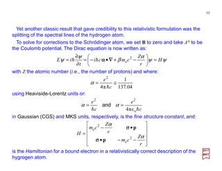
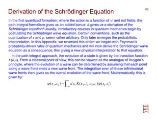
35. For example, consider the Green function for the Schrödinger equation:
If we take the Fourier transform of this equation and solve for the Green function, we
get:
35
2017
MRT
)()( 4
00 xxxxGH
t
i ′−=′−





−
∂
∂
δ
∫
′−⋅−
−
=′− )(
24
4
0 e
2ω
1
)π2(
)( xxpi
m
xd
xxG
pk
where pµ =[ωk,p]. This expression also suffers from an ambiguity, because the
integration over the energy, ωk, is divergent.
Let us take the convention that we integrate over the real axis (see Figure), so that we
integrate above the singularity. This can be accomplished by inserting a factor of iε into
the denominator, replacing ωk −p2/2m with ωk −p2/2m+iε. Then the ωk integration can be
performed.
Contour integration for the Green function. (Left) The contour gives us the nonrelativistic retarded Green
function. (Right) Contour giving the Feynman prescription for a relativistic (ωk ≡√(k2 +m2)) Green function.
p2/2m
Im k0Im ωk
Re k0Re ωk−ε −ε
ωk+ε

36. We simply convert the integration over the real axis into a contour integration over the
complex variable ωk. We are going to add the contour integral over the upper half plane
(which vanishes) such that:
where the θ function has been written as:
xpi
p x ⋅−
= e
)π2(
1
)( 23
φ
36
2017
MRT
∫∫ ∫ ′−−=
+−
=′− ′−−′•
∞+
∞−
′−−
′•
)(e
)π2(2ω
e
π2
ω
e
)π2(
)( ))(2()(
3
3
2
)(ω
)(
3
3
0
2
tt
d
i
εim
dd
xxG ttmii
tti
i
θpxxp
k
kxxp p
p
p k
−−−−−−−−


 ′>
=
+
−=′− ∫
∞+
∞−
′−−
→ otherwise
if
0
1
ω
e
ω
π2
1
lim)(
)(ω
0
tt
εi
d
i
tt
tti
ε k
k
k
θ
which equals 1 for t >t′, and vanishes otherwise.
To see this a bit more explicitly, let us define:
so that the Green function can be written as:
∫ ′′−−=′− )()()()( *3
0 xxdttixxG pp φφθ p
where φp(x) above correspond to a formulation based on the plane wave approximation.
In this way, the +iε insertion has selected out the retarded Green function, which obeys
the usual concept of causality. Taking the −iε prescription would have given us the
advanced Green function, which would violate causality.

37. Finally, taking the d3p integration (which is Gaussian integral), we find the final result
for the Green function (c.f., Appendix II: Path Integrals):
which is just the Green function found in ordinary quantum mechanics – a result we
obtained in PART III – QUANTUM MECHANICS using other means.
37
2017
MRT
)(e
)(π2
)(
2
2
23
0 tt
tti
m
ixxG tt
m
i
′−





′−
−=′− ′−
′
−
θ
xx−−−−

38. Now that we have seen how various prescriptions for iε give us various boundary
conditions, let us apply this knowledge to the relativistic case and choose the following,
unorthodox prescription:
To see how this iε prescription modifies the boundary conditions, we will find it useful to
decompose this as:
38
2017
MRT
εimk
kF
+−
=∆ 22
1
)(








−++
+
++−
=
+− εimkεimkkεimk 220220022
11
2
11
kk
The integral over k0 now picks up contributions from both terms. Performing the
integration as before (c.f., Klein-Gordon Scalar Field chapter), we find:
∫∫
∫∫
′−′−′′−−=
−′−′−−=′−∆ ′−⋅′−⋅−
)()(
ω2)π2(
)()()(
ω2)π2(
)(
e
ω2)π2(
)(e
ω2)π2(
)()(
*
3
3
*
3
3
)(
3
3
)(
3
3
xx
d
ttixx
d
tti
d
tti
d
ttixx
pppp
xxkixxki
F
φφθφφθ
θθ
kk
kk
kk
kk
We see the rather unusual feature of this prescription: positive energy solutions
are carried forward in time, but negative energy solutions are carried backwards in
time!

39. In classical physics, the usual solutions of the Maxwell theory give us retarded and
advanced waves, and we eliminate the advanced waves by a choice of boundary
conditions. However, in the quantum theory we are encountering a new type of
propagator that, classically, makes no sense, with negative energy solutions going
backwards in time. This propagator never appears in classical physics because it is
complex and hence forbidden classically.
Quantum mechanically though, negative energy solutions are an inherent problem with
any relativistic theory. Even if we ban them at the beginning, quantum interactions will
inevitably re-create them later! However, as we saw in the previous chapter (c.f., the
Pauli-Weisskopf interpretation of negative probabilities in the Charged Scalar chapter),
these negative energy states can also be reinterpreted. Feynman’s approach to this
problem was to assume that these negative energy states, because they are going back
in time, appear as a new form of matter with positive energy going forward in time,
antimatter! Although matter going backwards in time seems to contradict causality, this
poses no problem because one can show that, experimentally, a system where matter is
going backwards in time is indistinguishable from antimatter going forward in time. For
example, an electron placed in an electric field may move to the right; however, if it is
moving backwards in time, it appears to move to the left. However, this is
indistinguishable experimentally from a positively charged electron moving forwards in
time to the left. In this way, we can interpret this theory as one in which everything (i.e.,
matter plus antimatter) has positive energy.
39
2017
MRT

40. Now, the previous expression for the Green function was written in terms of plane
waves φp. However, we can replace the plane wave φp by the quantum field φ(x) if we
take the vacuum expectation value (i.e., 〈0|…|0〉) of the product of fields (i.e., φ(x)φ(x′)).
From the previous equation for the propagator ∆F(x−x′), we find:
where T is called the time-ordered operator, defined as:
40
2017
MRT
0)]()([0)( xxTxxi F ′=′−∆ φφ



>′′
′>′
=′
ttxx
ttxx
xxT
if
if
)()(
)()(
)]()([
φφ
φφ
φφ
So, the operator T makes sure that the operator with the latest time component always
appears to the left (mnemonic: lt-lt) This equation for ∆F is our most important result for
propagators. It gives us a bridge between the theory of propagators, in which scattering
amplitudes are written in terms of ∆F(x−x′), and the theory of operators, where
everything is written in terms of the quantum field φ(x).

41. Finally, we remark that our theory must obey the laws of causality. For our purposes,
we will define microscopic causality as the statement that information cannot travel
faster than the speed of light. For field theory, this means that φ(x) and φ(y) cannot
interact with each other if they are separated by space-like distances. Mathematically,
this means that the commutator between these two fields must vanish for space-like
separations.
Repeating the earlier steps, we can show that this commutator equals:
41
2017
MRT






−<−−
<<−
>−
∂
∂
=
−=
−∆=
∫
−⋅−
rtrtmJ
rtr
rtrtmJ
rr
i
kmkkd
yxiyx
yxki
if
if
if
)(
0
)(
π4
e)()(
)π2(
1
)()](,)([
22
0
22
0
)(
0
224
23
εδ
φφ
where ε (k) equals +1 (−1) for positive (negative) k, t=x0 −y0, r=|x−−−−y|, and J0 is the Bessel
function. With this explicit form for the commutator, we can easily show that, for space-
like separations, we have:
( )0)(0)( 2
<−=−∆ yxyx if
This shows that our construction obeys microscopic causality.

42. After Dirac considered the relativistic theory of radiation in 1927, he set out the next year
to construct the relativistic theory of electrons. One severe limitation was the problem of
negative probabilities. He started with the observation that the nonrelativistic
Schrödinger equation did not have negative probabilities because it was linear in time,
while the Klein-Gordon equation, being quadratic in time, did have negative probabilities.
Therefore Dirac tried to find a wave equation that was linear in time but still satisfied
the relativistic mass-shell constraint:
2222
mEppp =−=≡ pµ
µ
Dirac Spinor Field
42
2017
MRT
Dirac’s original idea was to take the square-root of the energy equation. In this way, he
stumbled onto the spinorial representation of the Lorentz group…
ψ
ψ
H
t
i =
∂
∂
where H is the Hamiltonian (e.g., H=T=p2/2m=−(1/2m)∇2 with p=−i∇∇∇∇, the quantum
momentum operator in h≡1 units).
Schrödinger’s time-dependent equation for a free particle of mass m is:
ψβα
ψ
)( mi
t
i i
i +∇−=
∂
∂
where αi (with summation implied over i=1,2,3) and β are now constant matrices,
not ordinary c-numbers, which act on ψ, a column matrix.
Dirac began with a first-order equation:

43. By squaring the operator in front of the ψ field, we want to recover the mass-shell
condition p2 = m2:
This is only possible if we demand that the matrices satisfy:
43
2017
MRT
ψ
ψβ
ψ
)(
)(
22
2
2
2
m
mi
t
+−∇=
+•−=
∂
∂
− ∇∇∇∇αααα
0},{
2},{
=
=+≡
βα
δαααααα
i
kiikkiki ,
To make the equations more symmetrical, we can then define γ 0 =β and γ i =βαi.
Multiplying the wave equation by β, we then have the celebrated Dirac equation:
0)( =−∂ ψγ µ
µ
mi
where the γ µ matrices satisfy:
νµνµ
ηγγ 2},{ =
It is no accident that such a relativistic construction is possible since this is
precisely the Clifford algebra which are formed by the γ µ. What we are really
constructing is the spin-½ representation of the Lorentz group, that is, the spinors.
and
122
== βαi

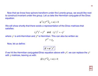
44. To calculate the behavior of this equation under the Lorentz group, let us define how a
Dirac spinor transforms under some (similarity) representation S(Λ) of the Lorentz group:
Then the Dirac equation transforms as follows:
)()()( xSx ψψ Λ=′′
44
2017
MRT
0)(])()([ 1
=−∂Λ=−∂ΛΛ−
ψγψγ ν
ν
µ
µ
µ
µ
mimSSi
where we have multiplied the transformed Dirac equation by S−1(Λ) on the left, and we
have taken into account the transformed ∂′µ=Λµ
ν ∂ν . In order for the above equation to
be Lorentz covariant, we must therefore have the following relation:
νµ
ν
µ
γγ ][)()( 11 −−
Λ=ΛΛ SS
To find an explicit representation for S(Λ), let us introduce the following matrix:
],[
2
νµνµ γγ
i
=Σ
The ½Σµν are the generators of the Lorentz group in this representation. Thus, we can
write a new Lorentz group generator that is the sum of the old generator Jµν =xµ pν −xν pµ
=i(xµ ∂ν −xν ∂µ) (which acts on the space-time coordinates xµ) plus a new piece that also
generates the Lorentz group but in the spinorial representation:
νµνµνµ Σ+=
2
1
JM
The Σµν also obey the [γ µ,Σρσ ]=2i(δρ
µγσ −δσ
µγρ) relation which shows that the Dirac
matrices transform as vectors under the spinor representation of the Lorentz group.

45. In terms of this new Mµν matrix, we can find an explicit representation of the S(Λ)
matrix:
νµ
νµ
Σ−
=Λ
ω)4(
e)(
i
S
45
2017
MRT
For example, consider a rotation R around the z-axis through an angle θ. Then:












−
=
θθ
θθ
θ
cos00sin
0100
0010
sin00cos
)(zR
and, for an infinitesimal transformation, θ <<1:
2112 ωω −=
and all other ωµν =0. Since M12 =−M21 =½γ1γ2, we obtain:






+





==Λ
2
sin
2
cose 21
)2( 21
θ
γγ
θθγγ
ii
and






−





==Λ −−
2
sin
2
cose 21
)2(1 21
θ
γγ
θθγγ
ii
With the help of Pauli matrices (e.g., σz), these can be written as Λ=exp(iσzθ/2). In
general, for a rotation through and angle θ around the direction n, Λ=exp(iσσσσ•nθ/2).ˆ ˆ

46. Let us look at a specific example of an infinitesimal expression for S. Consider a boost
in the x-direction with v=tanhζ. Then, we have:












−
−
=Λ=Λ
1000
0100
00coshsinh
00sinhcosh
]01[ ζζ
ζζ
ν
µ
46
2017
MRT
which, using Λµ
ν =δ µ
ν +εωµ
ν , implies that:
ν
µ
ν
µ ζεζεε M=












−
−
=
0000
0000
0001
0010
ω
where the matrix actually represents M01, one of the generators of the Poincaré group. In
general though, if M=Mµ
ν , then M2 =diag(1,1,0,0), M3 =M, M4 =M2, &c. Thus, we have:
µν
µ
ζµ
α
µ
ν
α
µν
µ
ν
ζδζδ xxM
N
M
N
xx M
N
N
]e[
11
lim
1
=














+





+=Λ=′
∞→
L

47. Now this last result means that:
47
2017
MRT
Note that the series contain only terms proportional to 1, M, and M2 and that it cuts
thereafter, which is due to the special form of the matrix M. Now, we have for a boost in
the x-direction:






−





=Λ
2
sinh
2
cosh)]([ 10
]01[ ζ
γγ
ζ
ζ 1S
and since Σ01=½i[γ0,γ1]=iγ0γ1 (i.e., with (−γ0γ1)2 =γ0γ1γ0γ1 =−γ0
2γ1
2 =1 since γ0γ1 =−γ0γ1,
γ0
2 =1 and γ1
2 =−1), so that:
]01[22
1
sinhcosh
!
e Λ=++−=+= ∑
∞
=
ζζ
ζζ
MMM
N
M
N
NN
M
11
01)2(]01[
e)]([
Σ
=Λ
ζ
ζ
i
S
10)2(]01[
e)]([ γγζ
ζ −
=ΛS
Therefore, using exp(ζ M)=1− M2 + M2coshζ + Msinhζ above, we can write the expression
for S as:
In general, for a boost in the xi-direction, we have:






−





=Λ
2
sinh
2
cosh)]([ 0
]0[ ζ
γγ
ζ
ζ i
i
S 1

48. Now, instead of boosts, we could have rotations such as a rotation R around the z-axis
through an angle θ just like before, which has:
48
2017
MRT
Thus, in this case, we obtain:
12)2(
e)]([
Σ
=
θ
θ
i
zRS
and since Σ12=½i[γ1,γ2]=iγ1γ2 (i.e., with (iγ1γ2)2 =−γ1γ2γ1γ2 =γ1
2γ2
2 =1), so that:
21)2(]01[
e)]([ γγθ
ζ ii
S =Λ






−





=





−





=
2
sin
2
cos
2
sinh
2
cosh)]([ 2121
θ
γγ
θθ
γγ
θ
θ 11 iiiRS z
where we used the identities cosh(ix)=cosx and sinh(ix)=isinx (for x real) in the last step.
Similarly, for a rotation about the xk-axis, we find (for cyclic permutations of i, j,k=1,2,3):






−





=
2
sin
2
cos)]([
θ
γγ
θ
θ jikRS 1
so that:






−





=





−





=
2
sin
2
cos)]([
2
sin
2
cos)]([ 132321
θ
γγ
θ
θ
θ
γγ
θ
θ RSRS ,
and






−





=
2
sin
2
cos)]([ 213
θ
γγ
θ
θRS

49. 49
2017
MRT
0)( ††
=+∂ mi µ
µ
γψ
s
We will show shortly that there exists a representation of the Dirac matrices that
satisfies:
ii
γγγγ −== †0†0
)()( and
where γ i is anti-Hermitian and γ 0 is Hermitian. This can also be written as:
Now that we know how spinors transform under the Lorentz group, we would like next
to construct invariant under the group. Let us take the Hermitian conjugate of the Dirac
equation:
µ
µ
γγ =†
Now, let us define:
If we hit the Hermitian conjugated Dirac equation above with γ 0, we can replace the γ †
with γ matrices, leaving us with:
0†
γψψ ≡
0)( =+∂ mi µ
µ
γψ
s

50. Under a Lorentz transformation, this new field ψ obeys:
50
2017
MRT
−
)()()]([)()( 10†0
Λ=Λ=′′ −
SxSxx ψγγψψ
This is just what we need to form invariants and covariant tensors. For example, notice
that ψψ is an invariant under the Lorentz group:−
)()()()()()()()()()( 1
xxxSSxxxxx ψψψψψψψψ =ΛΛ=′′′′=′′′′ −
1
since S −1(Λ)S(Λ)=1. Similarly, ψ γ µψ is a genuine vector under the Lorentz group. We
find:
−
)()()()()()()()( 1
xxxSSxxx ψγψψγψψγψ νµ
ν
µµ
Λ=ΛΛ=′′′′ −
where we have used the fact that S −1(Λ)γ µ S(Λ)=Λµ
ν γ ν which is nothing but the
statement that the γ µ transform as a vector under the spinor representation of the
Lorentz group.
In the same manner, it can also be shown that ψ Σµνψ transforms as a genuine
antisymmetric second-rank tensor under the Lorentz group.
−

51. To find other Lorentz tensors that can be represented as bilinears in the spinors, let us
introduce the matrix:
where ε µνρσ =−εµνρσ and ε 0123 =+1. Because γ5 transforms like ε µνρσ , it is a pseudoscalar
(i.e., it changes sign under a parity transformation). Thus, ψ γ5ψ is a pseudoscalar.
σρνµ
σρνµ γγγγεγγγγγγ
!4
32105
5
i
i −=≡=
51
2017
MRT
−
In fact, the complete set of bilinears, their transformation properties, and the number of
elements within each tensor are given by:
]6[
]4[
]4[
]4[
]1[
5
5
ψψ
ψγγψ
ψγψ
ψγψ
ψψψψ
νµ
µ
µ
Σ
=
:Tensor
:vector-Axial
:Vector
:arPseudoscal
:Scalar 1
There is a total of 16 independent components in the list.

52. The following set Γ of 16 matrices are linearly independent:
52
2017
MRT
},,,,{ 55 νµµµ
γγγγ Σ=Γ 1A
where A=1,2,…,16 and note that:
321
15
210
14
130
13
320
12
30
11
20
10
10
9
21
8
13
7
32
6
3
5
2
4
1
3
0
2
441
γγγ
γγγγγγγγγ
γγγγγγ
γγγγγγ
γγγ
γ
i
iii
iii
iii
I
=Γ
=Γ=Γ=Γ
=Γ=Γ=Γ
=Γ=Γ=Γ
=Γ=Γ=Γ
=Γ
≡=Γ ×
,,,
,,,
,,,
,,,
,
,1
and
53210
16 γγγγγ ≡=Γ i
and
Specifically, these Γ matrices are:
1≡Γ 2
)( A
ABBA ΓΓ±=ΓΓ

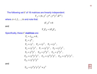
53. Because γ µ transforms as a vector under the Lorentz group, the following Lagrangian
is invariant under the Lorentz group:
This, in turn, is the Lagrangian corresponding to the Dirac equation, LDirac. Variations of
this equation by ψ or by ψ will generate the two versions of the Dirac equation.
µνσ
ρ
σνµρνµ
ρ
νµρµ
ρ
µρ
µ
µ
γγγγγγγγηγγγγγγγγγγ 2424 −==−== and,,
53
2017
MRT
ψγψ µ
µ
)(Dirac mi −∂=L
−
Up to now, we have not said anything specific about the representation of the Dirac
matrices themselves. In fact, a considerable number of identities can be derived for
these matrices in four dimensions, without even mentioning a specific representation,
such as:
Some trace operations can also be defined:
σρνµσρνµ
ρνσµσνρµσρνµσρνµ
νµνµνµνµµ
εγγγγγ
ηηηηηηγγγγ
ηγγγγγγγ
i4)(Tr
)(4)(Tr
4)(Tr0)(Tr)(Tr)(Tr
5
55
=
+−=
===Σ=
and
,,
In particular, this means:
where the Feynman slash notation is used:
µ
µ
γ aa ≡/
)])(())(())([(4)(Tr cbdadbcadcbadcba ⋅⋅+⋅⋅−⋅⋅=////

54. It is often convenient to find an explicit representation of the Dirac matrices. The most
common representation of these matrices is the Dirac representation:
where σ i are the familiar Pauli spin matrices (c.f., Appendix III: Dirac Matrices). Then the
spinor ψ is a complex-valued field with four components describinga massive spin-½ field!








=





−
=








−
=





−
=
0
0
10
01
0
0
10
010
i
i
i
i
i
i
σ
σ
αβ
σ
σ
γγ and,,
54
2017
MRT
Now let us try to decompose ψ(x) into plane waves in order to begin the canonical
quantization process… To do this, we need to find a set of independent basis spinors for
ψ. We will make the obvious (i.e., a ‘1’ in a column vector, a unit spinor, &c.) choice:












=












=












=












=
1
0
0
0
)0(
0
1
0
0
)0(
0
0
1
0
)0(
0
0
0
1
)0( 2121 vvuu ,and,
The trick is to act upon these basis spinors with S(Λ) in order to boost them up from zero
(i.e., p=k=0) to arbitrary momentum p. The momentum-dependent spinors are given by:
)0()()()0()()( αααα vSpvuSpu Λ=Λ= and
with the spinor indices α =1,2. This last set of equations can be shown to obey:
0)()(0)()(0)()(0)()( =+⋅=−⋅=+⋅=−⋅ mppvmppupvmppump γγγγ &,,

55. The Lorentz transformation (similarity) matrix S(Λ) is not difficult to construct if we set
all rotations to zero, leaving us with only Lorentz boosts. Then the only generators we
have are the K generators:
where:










+
•
+
•
+
=
























•






•





=Λ
1
p
p
1
p
p
mE
mE
m
mE
S
σσσσ
σσσσ
σσσσ
σσσσ
2
2
cosh
2
sinhˆ
2
sinhˆ
2
cosh
)(
ζζ
ζζ
55
2017
MRT
m
mE
m
mE
22
sinh
22
cosh
−
=




+
=




 ζζ
and
which in turn are proportional to σ i ≡σσσσ. Specifically, we have:








=== k
k
kjiiii i
MK
σ
σ
εγγ
0
0
2
1
],[
4
00
and p≡p/|p| is a unit vector in the direction of the 3-momentum p.ˆ

56. Applying S(Λ) to the independent spinor basis, we find:
56
2017
MRT
,,


















+
−
+
−+
=


















+
+
+
+
=
mE
p
mE
pip
m
mE
pu
mE
pip
mE
p
m
mE
pu
z
yx
yx
z
1
0
2
)(
0
1
2
)( 21
So, because of the particular decomposition we have chosen, the u spinors
correspond to electrons with positive energy (i.e., moving forward in time), while
the v spinors correspond to electrons with negative energy (i.e., moving backwards
in time). That being said, electrons with negative energy are known as positrons!
and


















+
−
+
−
+
=


















+
+
+
+
=
1
0
2
)(
0
1
2
)( 21 mE
p
mE
pip
m
mE
pvmE
pip
mE
p
m
mE
pv
z
yx
yx
z
,

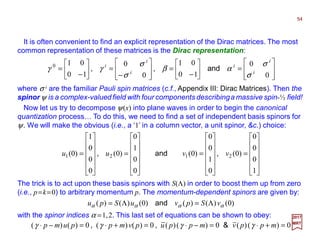
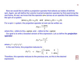
57. Next, we would like to describe spinors of definite spin. In many experiments, we can
produce polarized beams of electrons; so it becomes important to understand how to
incorporate projection operators that can select definite spin. This is not as simple as
one might suspect, since the intuitive concept of spin is rooted in our notion of the
rotation group (i.e.,O(3)), which is only a subgroup of the Lorentz group (i.e.,SO(1,3)).
In the rest frame, however, we know that the spin of a system can be described by a
three-vector s that points in a certain direction; so we may introduce the four-vector sµ
which, in the rest frame, reduces to sµ =[0,s]. Then, by demanding that this transform as
a four-vector, we can boost this spin vector by a Lorentz transformation Λ. Since we
define s2 =1, this means that sµ
2 = −1. In the rest frame, we have pµ =[m,0] (N.B., m=mo,
the rest mass) so we also have pµ sµ = 0, which must also hold in any boosted frame by
Lorentz invariance. Thus, we now have two Lorentz-invariant conditions on the spin four-
vector:
012
=−= µ
µµ sps and
57
2017
MRT

58. Now we would like to define a projection operator that selects out states of definite
spin. Again, we will define the Lorentz invariant projection operator by first examining the
rest frame. At rest, we know that the operator σσσσ •s serves as an operator that determines
the spin of a system:
where the + refers to the u spinor, and − refers to the v spinor.
2
1
)(
s
s
•±
=
σσσσ
P
58
2017
MRT
)0()0()()0()0()( αααα vvuu −=•=• ss σσσσσσσσ and
For a spin-½ system, the projection operator at rest can be written as:
2
1
)(
5
γµ +
≡sP
where γ 5 = iγ 0γ 1γ 2γ 3.






•−
•+
=→
s
s
s
σσσσ
σσσσ
10
01
2
1
)()( PsP µ
Therefore, this operator reduces to the previous one, so this is the desired
expression.
In the rest frame, this projection reduces to:
Our goal is to write a boosted version of this expression. Let us define the projection
operator :

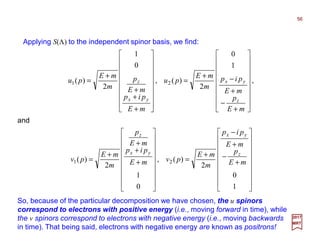
59. The new eigenfunctions now have a spin s (a quantum number) associated with them:
These spinors are quite useful for practical calculations because they satisfy certain
completeness relations. Any four-spinor can be written in terms of linear combinations of
the four uα(0) and vα(0) because they span the space of four-spinors. If we boost these
spinors with S(Λ), then uα(p) and vα(p) span the space of all four-spinors satisfying the
Dirac equation. Likewise, uα
T(0)vβ (0), &c. have 16 independent elements, which in turn
span the entire space of 4×4 matrices. Thus, uα
T(p)vβ (p), &c. span the space of all 4×4
matrices that also satisfy the Dirac equation.
0),()(),()(),(),()(),(),()( =−=−== skvsPskusPskvskvsPskuskusP and,
59
2017
MRT
−
We normalize our spinors with the following convention:
1),(),(1),(),( −== spvspvspuspu and
With these normalizations, these spinors obey certain completeness relations:
βαβαβα δ=−∑s
spvspvspuspu )],(),(),(),([
For the particular representation we have chosen, we find:
βα
βα
βα
βα
γγ





 /+−/−=




 /++/=
2
1
2
),(),(
2
1
2
),(),( 55 s
m
mp
spvspv
s
m
mp
spuspu and
They satisfy:
),()( skuku →

60. If we sum over the helicity s, we have two projection operators:
These projection operators satisfy:
102
=Λ+Λ=ΛΛΛ=Λ −+−+±± and,
60
2017
MRT
βα
βαβα 




 +/==Λ ∑±
+
m
mp
spuspup
s
2
),(),()]([
βα
βαβα 




 +/−
=−=Λ ∑±
−
m
mp
spvspvp
s
2
),(),()]([
and:
Because of the completeness relations, Λ± has a simple interpretation: It projects out the
positive or negative energy solution!

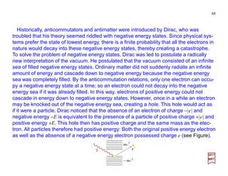
61. So far, we have only discussed the classical theory. To ‘second quantize’ the Dirac field,
we first calculate the momentum canonically conjugate to the spinor fieldψ :
Quantizing the Spinor Field
61
2017
MRT
since LDirac =ψ (iγ µ∂µ −m)ψ andψ =ψ †γ 0 the adjointofψ (N.B.,ψ † is the conjugate trans-
pose of ψ). Let us decomposethe spinor fieldψ (and its adjointψ )into Fourier moments:
†Dirac
)(
)( ψ
ψδ
δ
π i
x
x ==
&
L
∫ ∑=
⋅⋅−
+=
2,1
†
3
3
0
]e)()(e)()([
)π2(
)(
α
ααααψ xkixki
kvkdkukb
d
k
m
x
k
and
∫ ∑=
⋅−⋅
+=
2,1
†
3
3
0
]e)()(e)()([
)π2(
)(
α
ααααψ xkixki
kvkdkukb
d
k
m
x
k
In terms of particles and antiparticles, this particular decomposition gives the following
physical interpretation:




= ⋅+
⋅−
positronenergypositiveCreates
electronenergypositivesAnnihilate
xpi
xpi
pvpd
pupb
x
e)()(
e)()(
)( †
ψ
(N.B., Having d† create a positive energy positron can be viewed as annihilating a
negative energy electron since if you recall, the u spinors correspond to electrons with
positive energy while the v spinors correspond to electrons with negative energy).

62. Repeating the steps we took for the scalar particle (c.f., Klein-Gordon Scalar Field
chapter), we insert these equations and solve for the Fourier moments in terms of the
fields themselves:
where:
∫∫ == )()()()()()( 03†03
xUxdkbxxUdkb kk
α
α
α
α γψψγ kk ,
62
2017
MRT
and
∫∫ == )()()()()()( 03†03
xxVdkdxVxdkd kk ψγγψ α
α
α
α kk ,
xki
k
xki
k kv
k
m
xVku
k
m
xU ⋅⋅−
≡≡ e)(
)π2(
)(e)(
)π2(
)(
0
3
0
3
and
Now let us insert the Fourier decomposition back into the expression for the Hamiltonian:
∫ ∑
∫
∫∫
=
−=
∂=
−==
2,1
††3
0
0
03
33
)]()()()([
)(
)(
α
αααα
ψγψ
ψπ
kdkdkbkbdk
id
ddH
x
x
xx LH &
Here we encounter a serious problem. We find that the energy of the Hamiltonian
can be negative. There is, however, an important way in which this minus sign can
be banished…

63. For starters, let us define the canonical equal-time commutation relations of the
fields and conjugate fields with ‘anticommutators’, instead of commutators:
In order to satisfy the canonical anticommutation relations, the Fourier moments must
themselves obey anticommutation relations given by:
jiji tt δδψψ )(}),(,),({ 3†
yxyx −−−−=
63
2017
MRT
)(})(,)({)(})(,)({ 3
,
†3
,
†
kkkk ′=′′=′ ′′′′ −−−−−−−− δδδδ αααααααα kdkdkbkb and
Now, if we ‘normal order’ the Hamiltonian, we must also drop the infinite zero
point energy, and hence:
∫ ∑=
+=
2,1
††
0
3
)]()()()([
α
αααα kdkdkbkbkdH x
and
∫ ∑=
+=
2,1
††3
)]()()()([
α
αααα kdkdkbkbd kxP
Thus, the use of anticommutation relations and normal ordering nicely solves the
problem of the Hamiltonian with negative energy eigenvalues!
Furthermore, the d† operators can be interpreted as creation operators for
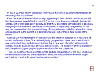
antimatter (or annihilation operators for negative energy electrons). In fact, this was
Dirac’s original motivation for postulating antimatter in the first place!

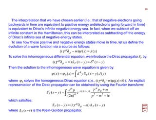
64. To see how this interpretation of these new states emerges, we first notice that the
Dirac Lagrangian is invariant under :
Therefore, there should be a conserved current associated with this symmetry. A direct
application of Noether’s theorem yields:
λλ
ψψψψ ii −
→→ ee and
64
2017
MRT
0=∂= µ
µ
µµ
ψγψ JJ and
which is conserved, if we use the Dirac equation.
Classically, the conserved charge is positive definite since it is proportional to ψ †ψ .
This was, in fact, an improvement over the classical Klein-Gordon equation, where the
charge could be negative. However, once we quantize the system, the Dirac charge can
also be negative. The quantized charge associated with this current is given by:
∫ ∑∫∫ =
−===
2,1
††3†303
])()()()([::
α
ααααψψ kdkdkbkbddJdQ xxx
This quantity can be negative, and hence cannot be associated with the probability
density. However, we can, as in the Klein-Gordon case, interpret this as the current
associated with the coupling to electromagnetism; so Q corresponds to the electric
charge. In this case, the minus sign in Q is a desirable feature, because it means that d†
is the creation operator of antimatter, that is, a positron with opposite charge to the
electron.

65. Again, this also means that we have to abandon the simple-minded interpretation of ψ
as a single-electron wave function, since it now describes both the electron and the
antielectron.
with only one particle in any given quantum state. This is the first example of the spin-
statistics theorem, that field theories defined with integer spin are quantized with
commutators are called bosons, while theories with half-integer spins are quantized
with anticommutators and are called fermions.
0)()(
1
†
1
†
j
M
j
i
N
i
kbkd ∏∏ ==
αα
65
2017
MRT
Now, the anticommutation relations also reproduce the Pauli Exclusion Principle
found in quantum mechanics. Because dα
†(k)dα
†(k)= 0, only one particle can occupy a
distinct energy state with definite spin. Thus, a multiparticle state is given by:
The existence of two types of statistics, one based on commutators (i.e., Bose-
Einstein statistics) and one based on anticommutators (i.e., Fermi-Dirac statistics),
has been experimentally observed in a wide variety of physical situations and has been
applied to explain the behavior of low-temperature systems and even which dwarf stars.

66. Repeating the same steps that we used for the Klein-Gordon field (c.f., Klein-Gordon
Scalar Field chapter), we can also compute the energy-momentum tensor, Tµν, and the
angular momentum tensor, Mλµν, from Noether’s theorem:
The conserved angular momentum tensor is therefore:
ψγψψγψψγψ νµµννµλνµµνλνµλνµνµ






Σ−∂−∂=





Σ−=∂=
22
i
xxi
i
JiiT Mand
66
2017
MRT
∫∫ 





Σ−∂−∂== ψψ νµµννµνµνµ
2
†303 i
xxiddM xx M
The crucial difference between these equations and the Klein-Gordon case is that the
angular momentum tensor contains an extra piece, proportional to Σµν, which represents
the fact that the theory has nontrivial spin-½.
We now calculate how a quantized spinor field transforms under the Poincaré group:
ψψψψ νµµννµνµ
µµ 





Σ−∂−∂=∂=
2
],[],[
i
xxMiPi and
With these operator identities, we can confirm that the quantized spinor field transforms
as a spin-½ field under the Poincaré group:
)()]([),(),( 11
axSaUaU +ΛΛ=ΛΛ −−
ββαα ψψ
which we have written in PART VI – GROUP THEORY as U(Λ,a)Ψα(x)U−1(Λ,a)=
D[Λ−1]α
β Ψβ(Λx+a). This closes the loop on the S(Λ) representation as being D[Λ].

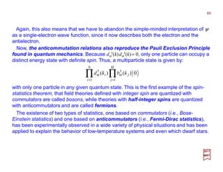
67. As we mentioned earlier, one of the fundamental assumptions about quantum field
theory is that it must be causal. Not surprisingly, the spin-statistics theorem is also
intimately tied to the question of microcausality, that is, that no signal can propagate
faster than the speed of light. From our field theory perspective, microcausality can be
interpreted to mean that the commutator (anticommutator) of two boson (fermion) fields
vanishes for spacelike separations:
To demonstrate the spin-statistics theorem, let us quantize bosons with anticommutators
and arrive at a contradiction. Repeating earlier steps, we find, for large separations:
( )0)(0])(,)([ 2
<−= yxyx forφφ
67
2017
MRT
2002
)(
)()(
23
3
)(
e
~
]ee[
ω2)π2(
0)}(,)({0
2002
yx
d
yx
yxm
yxkiyxki
−−
+=
−−−
−⋅−⋅−
∫
yx
k
yx
k
−−−−
−−−−
φφ
which clearly violates our original assumption of microcausality.
and
( )0)(0])(,)([ 2
<−= yxyx forψψ

68. Historically, anticommutators and antimatter were introduced by Dirac, who was
troubled that his theory seemed riddled with negative energy states. Since physical sys-
tems prefer the state of lowest energy, there is a finite probability that all the electrons in
nature would decay into these negative energy states, thereby creating a catastrophe.
To solve the problem of negative energy states, Dirac was led to postulate a radically
new interpretation of the vacuum. He postulated that the vacuum consisted of an infinite
sea of filled negative energy states. Ordinary matter did not suddenly radiate an infinite
amount of energy and cascade down to negative energy because the negative energy
sea was completely filled. By the anticommutation relations, only one electron can occu-
py a negative energy state at a time; so an electron could not decay into the negative
energy sea if it was already filled. In this way, electrons of positive energy could not
cascade in energy down to negative energy states. However, once in a while an electron
may be knocked out of the negative energy sea, creating a hole. This hole would act as
if it were a particle. Dirac noticed that the absence of an electron of charge −|e| and
negative energy −E is equivalent to the presence of a particle of positive charge +|e| and
positive energy +E. This hole then has positive charge and the same mass as the elec-
tron. All particles therefore had positive energy: Both the original positive energy electron
as well as the absence of a negative energy electron possessed charge e (see Figure).
68
2017
MRT
γ
−
e
2
mc
2
mc−

69. The interpretation that we have chosen earlier (i.e., that of negative electrons going
backwards in time are equivalent to positive energy antielectrons going forward in time)
is equivalent to Dirac’s infinite negative energy sea. In fact, when we subtract off an
infinite constant in the Hamiltonian, this can be interpreted as subtracting off the energy
of Dirac’s infinite sea of negative energy states.
To see how these positive and negative energy states move in time, let us define the
evolution of a wave function via a source as follows:
)()()( xJxmi =−∂ ψγ µ
µ
69
2017
MRT
To solve this inhomogeneousdifferential equation,we introduce the Dirac propagatorSF by:
)()()( 4
yxyxSmi F −=−−∂ δγ µ
µ
Then the solution to the inhomogeneous wave equation is given by:
∫ −+= )()()()( 4
0 yJyxSydxx Fψψ
where ψ0 solves the homogeneous Dirac equation (i.e., (iγ µ∂µ −m)ψ0(x)= 0). An explicit
representation of the Dirac propagator can be obtained by using the Fourier transform:
where ∆F (x−y) is the Klein-Gordon propagator.
which satisfies:
∫ +−
+
=− −⋅−
ε
γ µ
µ
imp
mppd
yxS yxpi
F 22
)(
4
4
e
)π2(
)(
)()()( yxmiyxS FF −∆−∂=− µ
µ
γ

70. As before, we can solve for the propagator by integrating over k0. The integration is
identical to the one found earlier for the Klein-Gordon equation, except now we have
additional γ µpµ + m factor in the numerator. Integrating out the energy, we can write the
Green function in terms of plane waves. The result is almost identical to the expression
found for the Klein-Gordon propagator, except for the insertion of γ matrices:
where:
70
2017
MRT
∫ ∑∑
∫








′−′+′′−−=
−′Λ+′−Λ−=′−
==
′−⋅
−
′−⋅−
+
4
3
2
1
3
)()(
3
3
)()()()()()(
)](e)()(e)([
)π2(
)(
r
pp
r
pp
xxpixxpi
F
xxttixxttid
ttpttp
d
E
m
ixxS
αααα
ψψθψψθ
θθ
p
p
xpir
p w
E
m
x ⋅−
≡
α
ε
αψ e)(
)π2(
1
)( 23
p
with ε α =(1,1,−1,−1) and w1 =u1, w2 =u2, w3 =v1, and w4 =v2. Written in this fashion, the
states with positive energy propagate forward in time, while the states with negative
energy propagate backwards in time.
0)]()([0)]([ yxTyxSi F βαβα ψψ=−
As in the Klein-Gordon case, we can now replace the plane waves ψp with the
quantized spinor ψ (x) by taking the vacuum expectation value of the spinor fields:
which is one of the most important results of this chapter.

71. For example, we can take an imaginary representation of the γ matrices, which gives
the Majorana spinors (c.f., Appendix III: Dirac Matrices). For our purpose, what is more
interesting is taking the Weyl representation, which gives us a representation of
neutrinos. If we take the representation:
Weyl Neutrinos
71
2017
MRT






−
=








−
=





−
−
=
10
01
0
0
01
10
5
0
γ
σ
σ
γγ and, i
i
i
then in this representation, we can write down two chiral operators:






=
+
≡
00
01
2
1 5γ
RP
and






=
−
≡
10
00
2
1 5γ
LP
The spinor representation of the Lorentz group is reducible if we introduce projection
operators PL and PR. Normally, we are not concerned with this because this spinorial
representation is irreducible under the full Poincaré group for massive states. However,
there is a situation when the spinorial representation becomes reducible even under the
Poincaré group, and that is when the fermion is massless.

72. To see how these projection operators affect the electron field, let us split ψ as follows:
Then we have:






=
L
R
ψ
ψ
ψ
72
2017
MRT






=




 −






=




 +
L
R
ψ
ψ
γψ
ψ
γ 0
2
1
02
1 55
and
Because PL and PR commute with the Lorentz generators (i.e., [PL,R,Σµν ]=0) it means
that the four-component spinor ψ actually spans a reducible representation of the
Lorentz group. Contained within the complex Dirac representation are tow distinct chiral
representations of the Lorentz group. Although ψL and ψR separately form an irreducible
representation of the Lorentz group, they do not form a representation of the Poincaré
group for massive particles. To find an irreducible representation of the Poincaré group,
we must impose m=0!
The reason that these chiral fermions must be massless is because the mass term
mψψ in the Lagrangian is not invariant under these two separate Lorentz
transformations. Because ψψ =ψLψR +ψRψL mass terms in the action necessarily mix
these two distinct representations of the Lorentz group. Thus, this representation forces
us to have massless fermions; that is, this is a theory of massless neutrinos.
−
− − −

73. The problem facing us now is to write down the action for the Dirac theory coupled to the
Maxwell theory, creating the quantum theory of electrodynamics, the subject of the rest
of this work. The most convenient way is to use the electron current as the source for
the Maxwell field. The electron current is given by J µ =ψ γ µψ (with ∂µ J µ =0 ‒ c.f.,
Quantizing the Spinor Field chapter), and hence we propose the coupling:
Relativistic Quantum Mechanics
73
2017
MRT
where e is the charge. We saw earlier that this current emerged because of the
invariance of the Dirac action under the symmetryψ ′→exp(iλ)ψ. Let us promote λ into a
local gauge parameter, so that λ is a function of space-time, λ(x). We want an action
invariant under:
ψγψ µ
µAe
−
)()(e)( )(
xAAxx xei
λψψ µµµ
λ
∂−→→ and
The problem with this transformation is that λ(x) is a function of space-time; therefore,
the derivative of a spinor ∂µψ is not a covariant object. It picks up an extraneous term
∂µdλ(x) in its transformation. To eliminate this extraneous term, we introduce the covariant
derivative:
µµµµ AeiD +∂≡→∂
The advantage of introducing the covariant derivative is that it transforms covariantly
under a gauge transformation:
)(e)()()(e)( )()(
xDxeixeixDxD xeixei
ψλλψψ µ
λ
µ
λ
µ →−+→

74. 2017
MRT
which we obtain by simply replacing ∂µ by Dµ .
74
This means that the following action is gauge invariant:
νµ
νµµ
µνµ
νµµ
µ
ψγψψγψ FFmDiFFmi
4
1
)(
4
1
)(EMDiracQED −−→−−∂=+= LLL
The coupling of the electron to the Maxwell field reproduces the coupling proposed
earlier. In the limit of velocities small compared to the speed of light, the Dirac equation
should reduce to a modified version of the Schrödinger equation. We are hence
interested in checking the correctness of the Dirac equation to lowest order, to see if we
can reproduce the nonrelativistic results and corrections to them. The Dirac equation of
motion, in the presence of an electromagnetic potential, now becomes:
To find solutions of this equation, let us decompose the four-spinor ψ into two smaller
two-spinors φ and χ:
ψβ
ψ
])([ 0
Aemei
t
i ++−•=
∂
∂
A−−−−∇∇∇∇αααα








Ψ
Φ
=





≡ −
−
tmi
tmi
e
e
χ
φ
ψ
Then the Dirac equation can be decomposed as the sum of two two-spinor equations:
χχφ
χ
φφχ
φ
mAe
t
imAe
t
i −+•=
∂
∂
++•=
∂
∂ 00
)()( ππππσσσσππππσσσσ and
where ππππ = p−eA is the canonical momentum and σσσσ represents the Pauli matrices.

75. Next, we will eliminate χ. For small fields, we can make the (first-order) approximation
that e A0 <<2m. Then we can solve the second equation as:
In this approximation, the Dirac equation can be expressed as a Schrödinger-like
equation, but with crucial spin-dependent corrections (i.e., the (e/2m)σσσσ •B term):
75
2017
MRT
φφχ <<
•
m2
~
ππππσσσσ
Φ








+•−=Φ








+
•
=
∂
Φ∂ 0
2
0
2
22
)(
2
)(
Ae
m
e
m
e
Ae
mt
i B
Ap
σσσσ
−−−−ππππσσσσ
where we have used the fact that:
B•−=• σσσσππππππππσσσσ e22
)(
The previous equation gives the first corrections to the Schrödinger equation in the
presence of a magnetic and electric field.

76. Classically, we know that the energy of a magnetic dipole in a magnetic field is given
by the dot product of the magnetic moment with the field:
the magnetic moment of the electron (with rest mass m=me) is therefore:
σσσσ
2
h
=S
76
2017
MRT
SS B
cm
e
cm
e
µ2
2
2
2 ee
=







=





≡ σσσσµµµµ
h
Thus, the Dirac theory predicted that the electron should have a magnetic moment
twice what one might normally expect, that is, twice the Bohr magneton µB. This was
perhaps the first major success of the Dirac theory of the electron. Historically, it gave
confidence to physicists that the Dirac theory was correct, even if it seemed to have
problems with negative energy states.
From the Stern-Gerlach experiment (1922), we know that (N.B., this is the meaning of
the ubiquitous and casual use of the term ‘spin-½’):
BBB •−=•−=•−= σσσσσσσσµµµµ
cm
e
cm
he
E
2π4
h
with the velocity of light c, the Planck quantum constant h, and the Dirac h-bar constant:
restored.
π2
h
≡h

77. Yet another classic result that gave credibility to this relativistic formulation was the
splitting of the spectral lines of the hydrogen atom.
in Gaussian (CGS) and MKS units, respectively, is the fine structure constant, and:
04.137
1
π4
2
≅=
c
e
h
α
77
2017
MRT
ψψ
α
β
ψ
ψ H
r
Z
cmci
t
iE =





−+•−=
∂
∂
= 2
e∇∇∇∇ααααhh
with Z the atomic number (i.e., the number of protons) and where:










−−•
•−
=
r
Z
cm
r
Z
cm
H
α
α
2
e
2
e
p
p
σσσσ
σσσσ
To solve for corrections to the Schrödinger atom, we set B to zero and take A0 to be
the Coulomb potential. The Dirac equation is now written as:
using Heaviside-Lorentz units or:
c
e
c
e
hh o
22
επ4
== αα and
is the Hamiltonian for a bound electron in a relativistically correct description of the
hygrogen atom.

78. In hindsight, it turn out to be convenient to introduce a judicious ansatz (i.e., an
educated guess that is verified later by its results) for the solution of the Dirac equation.
First, as in the Schrödinger case, we want to separate variables, so that we take:
where the radial function is explicitly separated off. Second, because ∇2 contains the
(Casimir) operator L2 in the usual Schrödinger formalism, we choose Y(θ,ϕ) to be the
standard spherical harmonics (i.e., eigenfunctions of the angular momentum operators).
For the spinning case, however, what appears is:
),()(~ ϕθψ Yrf
78
2017
MRT
2
σσσσ
++++++++ LSLJ ==
where J is the total spin, that is, the combination of the orbital spin L and intrinsic spin S.
Thus, our eigenfunctions for the Dirac case must be labeled by eigenvalues j, l, and ml.

79. Based on these arguments, we choose as our ansatz (i.e., an educated guess!):
Inserting this ansatz into the Dirac equation above and factoring out the angular part, we
find that the radial part of our eigenfunctions obey:
r
rF
j
rd
rFd
rG
r
Z
mE
jj
j
)(
2
1)(
)(e
ll
l m 





+−=





+−
α
79
2017
MRT












•
=
ll
ll
l
l
l
l
mj
j
mj
j
mj
r
rF
r
rG
i
φ
φ
ψ
)ˆ(
)(
)(
rσσσσ
r
rG
j
rd
rGd
rF
r
Z
mE
jj
j
)(
2
1)(
)(e
ll
l m 





+=





++
α
and
where we use the (E+… ((E−…) sign for j=l +½ ( j=l −½). For the interested reader
who would consult the References, you will see that by power expanding this equation
in r, this series of equations can be solved (although with quite some amount of
difficulty unless you’re a genius like Lev Landau) in terms of the confluent hypergeo-
metric function 1F1(a,b;z) (or Kummer’s function of the first kind).

80. These equations, when power expanded, give us the energy eigenstates of the
hydrogen atom (N.B., recall that the fine structure constant is given by α =e2/4π εohc):
Experimentally, this formula correctly gave spin-dependentcorrections to the Bohr formula
(i.e., En =−½mec2Z2α 2/n2) to lowest order. In contrast to the usual Bohr formula, the
energy is now a function of both the principal quantum number n as well as the total spin
j. By power expanding, we can recover the usual nonrelativistic result to lowest order:
21
2
222
2
e
)½()½(
1
−


















−+++−
+=
α
α
Zjjn
Z
cmE jn
80
2017
MRT








+





−
+
−−= L
4
3
½
)(
2
1
2
1
1 4
222
2
22
2
e
j
n
n
Z
n
Z
cmE jn
αα
So far, we have only considered the Dirac electron interacting with a classical Coulomb
potential. Therefore, it is not surprising that this formula neglects smaller quantum
corrections in the hydrogen energy levels. In particular, the 2S½ and 2P½ levels have the
same n and j values, so they should be degenerate according to the Dirac formula.
However, experimentally these two levels are found to be split by a smaller amount,
called the Lamb shift. It was not until 1949, with the correct formulation of the quantum
theory of electrodynamics (QED), that one could successfully calculate these small
quantum corrections to the Dirac energy levels. The calculation of these quantum
corrections in QED was one of the finest achievements of quantum field theory.

81. Because of gauge invariance, there are also complications when we quantize the theory.
A naïve quantization of the Maxwell theory fails for a simple reason: the propagator does
not exist! To see this, let us write down the action in the following form:
Quantizing the Maxwell Field
81
2017
MRT
where:
ν
νµ
µ
APA 2
2
1
∂=L
2
∂
∂∂
−=
νµ
νµνµ ηP
The problem with this propagator is that it is not invertible, and hence we cannot
construct a propagator for the theory. In fact, this is typical of any gauge theory, not just
Maxwell’s theory.
The origin of the noninvertibility of this operator is because Pµν is a projection
operator (i.e., its square is equal to itself, Pµν Pνλ =P λ
µ, and it projects out longitudinal
states, ∂µPµν =0). The fact that Pµν is a projection operator goes to the heart of why
Maxwell’s theory is a gauge theory. This projection operator projects out any states with
the form ∂µλ, which is just the statement of gauge invariance.

82. The solution to this problem is that we must break this invariance by choosing a
gauge. In our case, choosing a gauge means that we are making a particular choice of
the scalar and vector potentials. Because we have the freedom to add ∂µχ to Aµ, we will
choose a specific value of χ which will break gauge invariance. We are guaranteed this
degree of freedom if the variation δ Aµ =∂µχ can be inverted. There are several ways in
which we can fix the gauge and remove this infinite redundancy. We can, for example,
place constraints directly on the gauge field Aµ, or we may add the following term to the
action:
where ξ is arbitrary. We list some common gauges:
2
)(
2
1 µ
µ
ξ
A∂−
82
2017
MRT
∞=
=
=
=∂
=
=
=∇
ξ
ξ
ξ
µ
µ
:gaugeUnitary
:gaugeFeynman
:gaugeLandau
:gaugeLandau
:gaugeTemporal
:gaugeAxial
:gaugeCoulomb
1
0
0
0
0
0
0
3
A
A
A
Aii
Notice that there are two equivalent ways to represent the Landau gauge.

83. In the Coulomb gauge, one extracts out the longitudinal modes of the field from the
very start. To show that the gauge degrees of freedom allows us to make this choice, we
write down:
Solving for χ, we find:
0)( =•=′• χ∇∇∇∇++++∇∇∇∇∇∇∇∇ AA
83
2017
MRT
∫ ′•
′
′−=
•
∇
−=
)(
π4
1
1
3
2
xA
xx
x
A
∇∇∇∇
−−−−
∇∇∇∇
d
χ
Likewise, the Landau gauge choice means that we can find a χ such that:
2
∂
∂
−=
µ
µ
χ
A

84. To begin the process of canonical quantization, we will take the Coulomb gauge in
which only the physical states are allowed to propagate. Let us first calculate the
canonical conjugate to the various fields. Since A0 does not occur in the Lagrangian, this
means that A0 does not appear to propagate, which is a sign that there are redundant
modes in the action. The other modes, however, have canonical conjugates:
We write the Lagrangian as:
2
0
2
EM
4
1
4
1
jiiii FFEE −−−=L
84
2017
MRT
i
i
i
i
i
EAA
AA
=∂−−==== 0
0
0
0 &
&& δ
δ
π
δ
δ
π
LL
and
22
0
2
EM
4
1
2
1
4
1
jii FFF −=−= νµL
where Fµν
2=Fµν Fµν, &c. We introduce the independent Ei field via a trick. We rewrite the
action as:
By eliminating Ei by its equation of motion, we find Ei =−F0i . By inserting this value back
into the Lagrangian, we find the original Lagrangian back again. In vector form, with Aµ=
[A0,A] and Fµν = ∂µ Aν ‒∂ν Aµ, this equation reads:
22
0EM
4
1
2
1
jiFA −−•−•−= EEAE ∇∇∇∇&L

85. Then we write the Lagrangian for QED as:
where A0 is a Lagrange multiplier. If we solve for the equation of motion of this field, we
find that there is the additional constraint:
85
2017
MRT
ψγψ
ψγψ
µ
µ
µ
µ
νµ
)(
4
1
2
1
)(
4
1
22
0
2
QED
mDiFA
mDiF
ji −+−−•−•−=
−+−=
EEAE ∇∇∇∇&
L
ψγψρ 0e==•E∇∇∇∇:LawGauss’
Thus, Gauss’ Law emerges only after solving for the equation of motion of A0. If we now
count the independent degrees of freedom, we find we have only two degrees left, which
correspond to the two independent transverse helicity states. Of the original four
components of Aµ, we see that A0 can be eliminated by its equation of motion, and that
we can gauge away the longitudinal mode, therefore leaving us with 4−2=2 degrees of
freedom which means that massless states have two helicity states (N.B., these
correspond to a state where the Pauli-Lubanski tensor Wλ =½ε λµνσ Mµν Pσ ‒ c.f., PART
VI – GROUP THEORY ‒ is aligned parallel to the momentum vector and also aligned
antiparallel to the momentum vector).
)(),()(
2
1 0
0
22
ψγψψ eA −•−++−•−= EABEAE ∇∇∇∇LL &
or:

86. Intuitively, this means that a photon moving in the z-direction can vibrate in the x- and
y-direction, but not in the z-direction or the timelike direction. This corresponds to the
intuitive understanding of transverse photons. In the Coulomb gauge, we can reduce all
fields to their transverse components by eliminating their longitudinal components. Let
us separate out the transverse (⊥) and longitudinal (||) parts as follows:
where:
||EEE ++++⊥=
86
2017
MRT
ρ2
1
∇
= ∇∇∇∇||E
We see also that ∇×∇×∇×∇×E|| =0. If we insert this back into the Lagrangian, then we find that all
longitudinal contributions cancel, leaving only the transverse parts, except for the piece:
∫=
∇
=
yx
yyxx
yxE ||
−−−−
),(),(),(),(
π8
1
2
1
2
1 ††
33
2
2
2 tttt
dd
e ψψψψ
ρρ
The last term is called the instantaneous four-fermion Coulomb term, which seems
to violate special relativity since this interaction travels instantly across space. How,
we shall show at the end of the chapter that this term precisely cancels against
another term in the propagator, so Lorentz symmetry is restored.
Let us now solve for E|| in terms of ρ. Then we have:
ρ=•=• ⊥ ||0 EE ∇∇∇∇∇∇∇∇ and

87. If we impose canonical commutation relations, we find a further complication. Naïvely,
we might want to impose [Ai(x,t),πj (y,t)]=−iδijδ 3(x−−−−y). However, this cannot be correct
because we can take the divergence of both sides of the equation. The divergence of Ai
is zero, so the left-hand side is zero, but the right-hand side is not. As a result, we must
modify the canonical commutation relations as follows:
where the right-hand side must be transverse; that is:
87
2017
MRT
)(
~
)],(,),([ yxyx −−−−jiji ittA δπ −=
∫ 







−= ′•
2
)(
3
3
e
)π2(
~
k
k xxk ji
ji
i
ji
kkd
δδ −−−−
As before, our next job is to decompose the Maxwell field in terms of its Fourier
modes, and then show that they satisfy the commutation relations. However, we must be
careful to maintain the transversality condition, which imposes a constraint on the
polarization vector εεεε α(k). The decomposition is given by:
∫ ∑=
⋅⋅−
+=
2
1
†
0
3
3
]e)(e)([)(
2)π2(
)(
α
ααα xkixki
kakak
k
d
x εεεε
k
A
In order to reserve the condition that A is transverse, we take the divergence of this
equation and set it to zero. This means that we must impose:
βαβαα
δ=•=• εεεεεεεεεεεε and0k

88. By inverting these last relations, we can solve for the Fourier moments in terms of the
fields:
In order to satisfy the canonical commutation relation among the fields, we must impose
the following commutation relations among the Fourier moments:
88
2017
MRT
and
∫ •∂= ⋅
)()(e
2)π2(
)( 0
0
3
3
xk
k
d
ika xki
A
k αα
εεεε
t
∫ •∂−= ⋅−
)()(e
2)π2(
)( 0
0
3
3
†
xk
k
d
ika xki
A
k αα
εεεε
t
)(])(,)([ 3†
kk ′=′ −−−−δδ βαβα
kaka
Recall the operator:
BABABA )(∂−∂≡∂
t

89. Let us now insert this Fourier decomposition into the expression for the energy and
momentum:
After normal ordering, once again the energy is positive definite.
∫ ∑=
′−⋅−
⊥
+
=′=′−
2
1
2
)(
4
4
)()(
e
)π2(
0)]()([0)]([
α
α
ν
α
µνµνµ εε kk
εik
kd
ixAxATxxDi
xxki
F
89
2017
MRT
∫ ∑∫=
=+=
2
1
†3223
])()([ω)(
2
1
α
αα
kakaddH kBEx
and
∫ ∑∫ =
==
2
1
†33
)()(:)(:
α
αα
kakadd kkBExP ××××
This expression is not Lorentz invariant since we are dealing with transverse states.
This is a bit troubling, until we realize that Green functions are off-shell objects and
are not measurable. However, these Lorentz violating terms should vanish in the full
scattering matrix.
Finally, we wish to calculate the propagator for the theory. Again, there is a
complication because the field is transverse. The simplest way to construct the
propagator is to write down the time-ordered vacuum expectation value of two fields.
The calculation is almost identical to the one for scalar and spinor fields, except we have
the polarization tensor to insert:

90. To see this explicitly, let us choose a new orthogonal basis of four vectors, given by
εµ
1(k), εµ
2(k), kµ, and a new vector eµ =[1,0,0,0]. Any tensor can be power expanded in
terms of this new basis. Therefore, the sum over polarization vectors appearing in the
propagator can always be expanded in terms of the tensors gµν, eµ eν, kµ kν , and kµ eν. We
can calculate the coefficient of this expansion by demanding that both sides of the
equation be transverse. Then we get:
Fortunately, the noninvariant terms involving e can all be dropped. The terms
proportional to kµ vanish when inserted into a scattering amplitude. This is because the
propagator couples to two currents, which in turn are conserved by gauge invariance.
22
2
2222
2
1 )()(
))((
)(
)()(
kek
eek
kek
kkkkek
kek
kk
kk
−⋅
−
−⋅
+⋅
+
−⋅
−−=∑=
νµµννµνµ
νµ
α
α
ν
α
µ ηεε
90
2017
MRT
If we drop terms proportional to kµ in the propagator, we are left with:
xx ′−
′−
−=′−∆−=′−⊥
π4
)(
)0;()]([
tt
eemxxxxD FF
δ
η νµνµνµ
The first term is what we want since it is covariant. The second term proportional to eµ eν
is called the instantaneous Coulomb term. In any Feynman diagram, it occurs between
two currents, creating (ψ †ψ )∇−2(ψ †ψ ). This term precisely cancels the Coulomb term
found in the Hamiltonian when we solved for E|| above.

91. The purpose of this Appendix is to derive the basic Hamiltonian of electrodynamics sub-
ject to the requirement that the three-vector potential A satisfies the transversality con-
dition. We shall first show that it is always possible to consider a gauge transformation of
type Aµ → A′µ + ∂µ χ such that in the new gauge the transversality condition (e.g., Fourier
transforming this to ik•A(k,t)=0,the transversalitycondition for a wave with wavevectork):
91
2017
MRT
),(),(),(
),(1
),(),( oldnewold
0
new
0 ttAtA
t
t
c
tAtA xxx
x
xx χ
χ
∇∇∇∇++++=
∂
∂
−= and
is satisfied (i.e., the vector potential is a transverse vector function). But for now, we set:
Appendix I: Radiation Gauge
0),( =• txA∇∇∇∇
where:
∫ ′
′•′
′=
xx
xA
xx
−−−−
∇∇∇∇
π4
),(
),(
old
3 t
dtχ
We then have:
0)( oldnew
=•=• χ∇∇∇∇++++∇∇∇∇∇∇∇∇ AA
which shows that the transversality condition is satisfied for the new vector potential. On
the other hand, from Aµ −∂µ (∂ν Aν )= J µ (c.f., Maxwell’s Equation chapter), where J µ is
the charge-current density, which holds quite generally, we get for the A0 component:
ρ−=





∂
∂
+•
∂
∂
+
∂
∂
−∇
t
A
ctct
A
c
A 0
2
0
2
20
2 111
A∇∇∇∇
~

92. When the three-vector potential satisfies the transversality condition, it is seen that A0
is determined by Poisson’s equation:
92
2017
MRT
),(),(0
2
ttA xx ρ−=∇
which does not contain any time derivative. The solution to this differential equation
satisfying the boundary condition A0 →0 at infinity is:
∫ ′
′
′=
xx
x
xx
−−−−
),(
π4
1
),( 3
0
t
dtA
ρ
We wish to emphasize that A0 in this last relation is an instantaneous Coulomb potential
in the sense that the value of A0 at t is determined by the charge distribution at the same
instant of time; in particular, it should not be confused with the retarded Coulomb
potential:
∫ ′
−=′
′
′
′=
ctt
t
dtA
xxxx
x
xx
−−−−−−−−
),(
π4
1
),( 3
0
ρ
which we obtain by solving the d’Alembertian equation A0 =0 for A0. To summarize
what we have done so far: 1) we can always choose the vector potential so that the
transversality condition ∇∇∇∇•A=0 is satisfied; 2) if A satisfies the transversality
condition, the A0 is given by the instantaneous Coulomb potential integral above. The
gauge in which A satisfies ∇∇∇∇•A=0 and A0 is given by the integral above is called the
radiation (or Coulomb) gauge.

93. The total Hamiltonian for the charged particles and the electromagnetic field is given
by the space integral of:
93
2017
MRT
nInteractioMatterEM HHHH ++=
From the Hamiltonian density of the electromagnetic field, we have, from (c.f., Maxwell’s
Equation chapter):
)()(
2
1
)(
2
1
)(
)(
00
22
0
22
EM0
0
EM
EM
EBE
EBE
AA
AA
A
•+−−=
•−−=−∂
∂
=
∇∇∇∇
∇∇∇∇
ρ
δ
δ
µ
µ
L
L
H
where the last term of the last line is of no significance since is vanishes when we
evaluate H=∫d3x HEM. As for the interaction part of the Hamiltonian density, we write is
as:
µ
µ JA
c
1
nInteractio −=H
Combining these last two equations yields:
∫∫∫ •−−=+=+ JAxBExx 3223
nInteractioEM
3
nInteractioEM
1
)(
2
1
)( d
c
ddHH HH
At first sight this appears to be a very strange result because of the ρA0 term has
completely disappeared! We shall come back to this puzzle in a moment…

94. Our next step is to show that this last Hamiltonian (i.e., HEM +HInteraction) can be written
in a somewhat different form when we work in the radiation gauge. First, we recall that,
quite generally, the electric field E is derivable from:
94
2017
MRT
tc
A
∂
∂
−=
A
E
1
0 −−−−∇∇∇∇
We claim that in the radiation gauge the irrotational and solenoidal part of E, defined by:
⊥= EEE ++++||
0EE ==• ⊥ ||0 ××××∇∇∇∇∇∇∇∇ and
where:
are uniquely given by:
yc
A
∂
∂
−=−= ⊥
⊥
A
EE
1
0|| and∇∇∇∇
where the subscript ⊥ is to remind us of the transversality condition ∇∇∇∇•A=0. This can be
proved by noting: 1) the vector identity ∇∇∇∇××××(∇∇∇∇A0) vanishes; 2) the divergence of ∂A⊥/∂t
vanishes because of the transversality condition ∇∇∇∇•A=0; and 3) the decomposition of E
into E|| and E⊥ is unique.

95. Meanwhile, we can show that the space integral of |E|2 is actually given by:
95
2017
MRT
∫∫∫ += ⊥ 0
32323
Addd ρxExEx
in the radiation gauge.
∫
∫∫∫∫∫
+=
=•+=+•−=
⊥
⊥⊥⊥⊥
)(
)(2])(2[
2
||
23
2
||
3
0
3232
||0
2323
EEx
ExExExEEExEx
d
dAddAdd ∇∇∇∇∇∇∇∇
∫
∫∫∫∫
=
∇−•=•=
0
3
0
2
0
3
00
3
00
32
||
3
)()()(
Ad
AAdAAdAAdd
ρx
xxxEx ∇∇∇∇∇∇∇∇∇∇∇∇∇∇∇∇
Furthermore:
Combining these last two results, we see that the space integral of |E|2 is indeed given
by ∫d3x|E|2 =∫d3x|E⊥ |2 +∫d3xρA0 .
To prove this, we first note:

96. Coming back to the expression for the Hamiltonian given by HEM +HInteraction above, we
note that the ρA0-term which, we thought, had disappeared is actually buried in the
space integral of |E|2:
96
2017
MRT
∫ ∫∫ ′
′
′=
xx
xx
xxx
−−−−π4
),(),(
2
1
2
1 33
0
3 tt
ddAd
ρρ
ρ
Note, however, that the ρA0-term now appears with a factor ½.
∫∫ 





•−−−=+ ⊥⊥ AJxBEx
c
AddHH
1
2
1
)(
2
1
0
3223
nInteractioEM ρ
We are finally in a position to eliminate A0 altogether (or equivalently E||) from the
Hamiltonian. Using the instantaneous Coulomb potential integral for A0(x,t) above, we
can write the ρA0-term of HEM +HInteraction above as:
Hence:
∫ ∫∫∫ ′
′
′+•−








∂
∂
=+ ⊥⊥
⊥
xx
xx
xxAJxA
A
x
−−−−
××××∇∇∇∇−−−−
π4
),(),(
2
111
2
1 3332
2
3
nInteractioEM
tt
ddd
ctc
dHH
ρρ
or, in terms of A⊥, J and ρ only:
∫∫ ∫∫ ⊥⊥ •−
′
′
′−−=+ AJx
xx
xx
xxBEx 333223
nInteractioEM
1
π4
),(),(
2
1
)(
2
1
d
c
tt
dddHH
−−−−
ρρ
In this form the electrostatic potential A0 (or irrotational part of E) has been
completely eliminated in favor of the instantaneous Coulomb interaction.

97. We can now forget about the dynamical degrees of freedom associated with A0 or E⊥.
In quantizing the Maxwell field it is sufficient to quantize just the transverse potential A⊥
provided we work in the radiation gauge. This procedure was first advocated by E. Fermi
in 1932. Now, from our last two equations for HEM +HInteraction above, we see that the only
term in the interaction Hamiltonian which involves the electromagnetic potential explicitly
is the space integral of −(1/c)J•A⊥. In nonrelativistic quantum mechanics this is given
just by the difference:
97
2017
MRT
∑∑ −







− ⊥
j
j
jj
jj
j mc
e
m
2)(
2
)(
)(
2
1
2
1
pAp
As for the Coulomb part, we can use the familiar form:
∑=
j
j
je )( )(3
xx −−−−δρ
to obtain:
∑∑∫ ∫ −=
′
′
′
> j
jj
j
ji
ji
ji eeett
dd
)()(
2
)()(
33
π42
1
π4π4
),(),(
2
1
xxxxxx
xx
xx
−−−−−−−−−−−−
ρρ
The last term which represents the interaction of a charged particle with the
Coulomb field due to the same charged particle is infinite; hence, it is usually
dropped. However, in discussing the self-energy of the Dirac electron, it is necessary
to include the relativistic analog of this term through renormalization techniques.

98. 98
2017
MRT
Appendix II: Path Integrals
Contents
Introduction
Postulates of Quantum Mechanics
Derivation of the Schrödinger Equation
From First to Second Quantization
Generating Functionals
Schwinger-Dyson Equations
“One feels as Cavalieri must have felt calculating the volume of a pyramid before the invention of
calculus.” Richard Feynman, Space-Time Approach to Non-Relativistic Quantum Mechanics, Rev. Mod.
Phys. 20, 267 (1948), footnote 10.

99. Previously, we outlined how to quantize field theories with various spins using the
canonical quantization approach. However, for increasingly complex systems, such as
gauge theory (N.B., the path integral method is versatile enough to handle a variety of
different types of gauge theories), quantum gravity, and superstring theory, canonical
quantization proves to be a very clumsy formalism since manifest Lorentz invariance is
broken. Instead, we will explore a new method in this Appendix.
99
2017
MRT
Introduction
Perhaps the most powerful quantization method is the path integral approach, which
was developed by Feynman (c.f., A Space-Time Approach to Quantum Mechanics. Rev.
Mod. Phys. 20, 267 (1948)), based on an idea of Dirac (c.f., The Lagrangian in Quantum
Mechanics, Physik Z. Sov. Union 3, 64 (1933)). Now Dirac’s idea was based on looking
at the basic difference between classical mechanics and quantum mechanics. We know
that in classical mechanics a definite path in the xt-plane is associated with the particle’s
motion. But in quantum mechanics all possible paths must play roles including those
which do not bear any resemblance to the classical path. Yet this must somehow be
possible by reproducing classical mechanics in a smoother manner in the limit h→0.
Incidentally, if you are interested in a compilation of the key historical papers on QED
(e.g., the ones referred to above), then procure Selected Papers on Quantum
Electrodynamics, Ed. Julian Schwinger (1958) which is available through Dover
Publications.

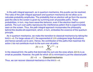
100. As the story goes, as a young graduate student at Princeton University working out the
problem of infinite self-energy of the electron (circa 1940), Feynman tried to attack this
problem using a least-action principle using half advanced and half retarded potentials.
The principle could deal successfully with the infinity arising in the application of classi-
cal electrodynamics. The problem then became one of applying this action principle to
quantum mechanics in such a way that classical mechanics could arise naturally as a
special case of quantum mechanics in the limit h→0. Feynman searched for any idea
which might have been previously worked out in connecting quantum-mechanical beha-
vior with such classical ideas as the Lagrangian or, in particular, Hamilton’s principle
function S, the action, the indefinite integral of the Lagrangian. During some conversa-
tions with a visiting European physicist, Feynman learned of a paper (c.f., ibid) in which
P. A. M. Dirac had suggested that the exponential function of iε times the Lagrangian
was analogous to a transformation function for the quantum-mechanical wave function in
that the wave function at one moment could be related to the wave function at the next
moment (a time interval ε later) by multiplying with such an exponential function [c.f., P.
A. M. Dirac, The Principles of Quantum Mechanics, 4-th Ed., P. 128 who provides the
following (edited) statement: “exp(iS/h) corresponds to the transition amplitude〈x2,t2|x1,t1〉,
where S is the action”]. Feynman attempted to make sense out of this remark. Is
analogous to [or corresponds to] the same thing as is equal to or is proportional to?
100
2017
MRT
Now, if you want to read a textbook dedicated to path integrals, then the authorita-
tive source is from the proverbial horse’s mouth: R. P. Feynman and A. R. Hibbs,
Quantum Mechanics and Path Integrals also available through Dover Publications.

101. Now back to the path integral approach.It has many advantages over other techniques:
101
2017
MRT
1. The path integral formalism yields simple, covariant quantization of complicated
systems with constraints, such as gauge theories. While calculations with the
canonical approach are often prohibitively tedious, the path integral approach yields
the results rather simply, vastly reducing the amount of work;
2. The path integral formalism allows one to go easily back and forth between the other
formalisms, such as the canonical or various covariant approaches. In the path inte-
gral approach, these various formalisms are nothing but different choices of gauge;
3. The path integral formalism is based intuitively on the fundamental principles of
quantum mechanics. Quantization prescriptions, which may seem rather arbitrary in
the operator formalism, have a simple physical interpretation in the path integral
formalism;
4. The path integral formalism can be used to calculate nonperturbative as well as
perturbative results;
5. The path integral formalism is based on c-number fields, rather than q-number
operators. Hence the formalism is much easier to manipulate;
6. At present, there are a few complex systems with constraints that can only be
quantized in the path integral formalism;
7. Renormalization theory is much easier to express in terms of path integrals.

102. Our discussion of the path integral formalism begins with Feynman’s Rules:
102
2017
MRT
2
),(),( abKabP =
The transition function from a single path is postulated to be an exponential whose
(imaginary) phase is the classical action (in units of h) for the path in question;
Postulates of Quantum Mechanics
1. The probability P(b,a) that a particle will arrive at b, when let out at the source a, can
be represented quantitatively by the absolute square of a complex number called the
transition function (or probability amplitude in Feynman’s language) K(b,a) – in this
case, the transition function that a particle from a will arrive at b is:
2. When a particle can reach a given state (say, point b) by two possible routes, the total
transition function for the process is the sum of the transition functions for the two
routes considered separately:
∑=++=
PathsAll
2Path1Path
e),(),(),( h
L Si
kabKabKabK
3. When a particle goes by some particular route b, the transition function for that route
can be written as the product of the transition function to go part way with the
transition function to go the rest of the way:
∑=
PathsAll
),(),(),( abKbcKacK
where k is a constant that can be determined by the rule 3, if applicable and;
where we sum over all intermediate point b connecting a and c.

103. These rules incorporate the essence of the celebrated double slit experiment, where a
beam of electrons passes through a barrier with two small holes. A screen is placed
behind the barrier to detect the presence of electrons (see Figure). As a point particle,
an electron cannot, of course, go through both holes simultaneously. Classically,
therefore, we expect that the electrons with go through one slit or the other, leaving two
distinct marks on the screen just behind the two holes. However, experiments show that
the pattern created on the screen by repeated passages of the electrons through these
holes is an interference pattern, associated with wave-like, not particle-like behavior.
Classically, we are therefore left with a paradox. A point particle cannot go through both
holes at once, yet the passage of a large number of electrons successively point past
the barrier clearly leaves an interference pattern, with minima and maxima, as if the
electron somehow went through both holes.
103
2017
MRT
Double Slit Observing screen over time
Individual
electron
Accumulated
individual
electrons
Emerging
interference
pattern
ElectronElectron gun
(Source)
Double-slit apparatus showing the pattern of electron hits on the observed screen building up over time.

104. In the path integral approach, as in quantum mechanics, this puzzle can be resolved.
The rules of the path integral approach and quantum mechanics do not allow us to
calculate probability amplitudes. The probability that an electron will go from the source
past the slits to the screen is given by summing over all possible paths. These
probabilities, in turn, may have wave-like behavior, even if the electron itself is a point
particle. The sum over paths reproduces the interference pattern that is experimentally
seen on the screen. Thus, the path integral approach incorporates the philosophy
behind the double-slit experiment, which, in turn, embodies the essence of the quantum
principle.
104
2017
MRT
0~e:
PathsAll
∑>> h
h Si
Sδ
As in quantum mechanics, we make the transition to classical mechanics by taking the
limit h→0. For large values of S, the exponential of iS/h undergoes large fluctuations,
and hence cancels out to zero. Hence, the contribution of the paths that maximize the
action S do not contribute much to the sum over all paths:
In the classical limit, the paths that dominate the sum are the ones where δ (S/h) is as
small as possible. However, the path for which δ S is minimized is just the classical path:
mechanicsClassical→= 0Sδ
Thus, we can recover classical mechanics in the limit h→0.

105. The picture that emerges from the path integral approach is therefore intuitively
identical to the principles of quantum mechanics. To calculate the probability that a
particle at point a goes to point b, one must sum over all possible paths connecting these
two points, including the classical one. The path preferred by classical mechanics is the
one that minimizes the action for δ S<<h.
105
2017
MRT
Although the path integral method gives us an elegant formalism in which to
reformulate all of quantum field theory, one should also point out the potential drawbacks
of the formalism. One problem is that the path integral is not well defined in Minkowski
space (i.e., ηµν =diag(1,−1,−1,−1)). In this Appendix, we will assume that all path integrals
are computed with the Euclidean metric (i.e., eij =diag(1,1,1)). Then, the functional
integral is taken over exp(−S), which has much better convergence properties that
integrals over exp(iS). At the end of the calculation, we assume that we can analytically
continue back to Minkowski space.
Another problem is that the transition between c-numbers and operators becomes ill-
defined when the Hamiltonian has ordering problems. The path integral over a system
with the Hamiltonian of the form p2 f (q), for example, becomes ambiguous when making
the transition to the operator language, since p and q do not commute. For systems
more complex than the harmonic oscillator, the integrals may not be Gaussian, and
ordering problems may creep into the path integral (e.g., for complicated systems, one
must often use point splitting methods, that is, separating two fields by a small
infinitesimal amount in space-time in order to regularize the integrals).

106. With these problems in mind, let us now compute with the path integral approach. We
first divide up a path by discretizing space-time. Let us divide up each path in three-
space into N points. Then the sum over all paths can be transformed into a functional
integral:
106
2017
MRT
∫∏∏∑ →≡
= =
∞→
xx
i
N
n
i
n
N
D
3
1 1PathsAll
lim δ
The integral ∫Dx is not an ordinary integral. It is actually an infinite product (i.e., using Πn
up to N→∞) of integrals, taken over all possible dx(t) (i.e., using Πi up to 3D Euclidean
space). So, whenever we use the differential symbol D, we should remember that it is
actually an infinite product of differentials taken over all points. In this functional
language, the transition function becomes:
∫= hSi
xkabK e),( D
where k can be determined as follows:
∫= ),(),(),( abKbcKxacK bD
where we integrate over all possible intermediate points xb which link points a and c.
From now on, we set h≡1.

107. To give this approach some substance, let us begin with the simplest of all possible
classical systems, the free nonrelativistic point particle in the first quantized formalism.
Our discussion begins with the classical action:
107
2017
MRT
∫= 2
2
1
ixmtdS &
so that the particle motion be solely kinetic in nature. Let us now discretize the paths.
We take dt to be a small interval ε and then discretize the Lagrangian:
ε
ε
2
12 )(
2
1
2
1 inn
i
xx
mtdxmtd +−
→→ &and
The transition function K(b,a) can be written as the path integral over exp(iS):
∫ ∫ ∫
∑
−
= +−
−
→
=
1
1
2
1)(
2
132
0
elim),(
N
n nn xx
mi
N kxdxdxdabK ε
ε
L
Man… What a mess! And this is for the simplest of all possible classical systems – you
say! Unfortunately, one of the drawbacks of the path integral formalism is that
embarrassingly few functional integrals can actually be performed.

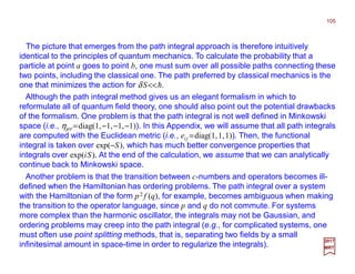
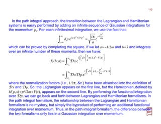
108. However, we will find that the simplest Gaussian path integral is also the one most
frequently found for free systems (i.e., those with the potential V(x) set to zero).
Specifically, we will repeatedly use the Gaussian integral:
108
2017
MRT
The key point is that the Gaussian integral over x2 has left us with another Gaussian
integral over the remaining variables. This process can be repeated an arbitrarily large
number of times: Each time we perform a Gaussian integral on an intermediate point, we
find a Gaussian integral among the remaining variables!
12
2 ½)(
e
22
+
∞
∞−
− +Γ
=∫ n
xrn
r
n
xxd
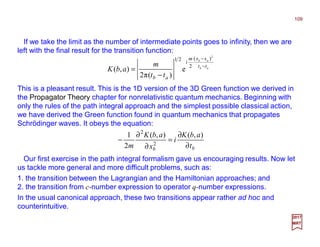
To evaluate the expression for K(b,a), we now perform one of these Gaussian
integrations:
2
312
32
2
21
)(
2
1
])()([
2 e
2
π
e
xxa
xxaxxa
a
xd
−−∞
∞−
−−−−
=∫
After repeated integrations, we find:
2
12
1
2
21
)(
1
1
2
2
])()([
12 e
)1(
π
e
N
NN
xxa
N
N
N
xxaxxa
N
aN
xdxd
−
−
−
−
−∞
∞−
−−−−−
−
−
=∫ −L
L
This, in turn, allows us to calculate the constant k:
2
π2
N
m
i
k
−






=
ε

109. If we take the limit as the number of intermediate points goes to infinity, then we are
left with the final result for the transition function:
109
2017
MRT
ab
ab
tt
xxm
i
ab tt
m
abK −
−
−
=
2
)(
2
21
e
)(π2
),(
This is a pleasant result. This is the 1D version of the 3D Green function we derived in
the Propagator Theory chapter for nonrelativistic quantum mechanics. Beginning with
only the rules of the path integral approach and the simplest possible classical action,
we have derived the Green function found in quantum mechanics that propagates
Schrödinger waves. It obeys the equation:
bb t
abK
i
x
abK
m ∂
∂
=
∂
∂
−
),(),(
2
1
2
2
Our first exercise in the path integral formalism gave us encouraging results. Now let
us tackle more general and more difficult problems, such as:
1. the transition between the Lagrangian and the Hamiltonian approaches; and
2. the transition from c-number expression to operator q-number expressions.
In the usual canonical approach, these two transitions appear rather ad hoc and
counterintuitive.

110. In the path integral approach, the transition between the Lagrangian and Hamiltonian
systems is easily performed by adding an infinite sequence of Gaussian integrations for
the momentum pi . For each infinitesimal integration, we use the fact that:
110
2017
MRT
∫
∫
∫
∫






−−






−
=
=
b
a
t
t
i
i
b
a
t
t
i
x
x
xV
m
p
xptdi
x
x
xVxmtdi
b
a
b
a
px
xabK
)(
2
)()(
2
1
2
2
e
e),(
&
&
DD
D
which can be proved by completing the square. If we let a=−1/2m and b=x and integrate
over an infinite number of these momenta, then we have:
a
b
i
pbipai
a
i
pd 4
2
22
e
π
e
−∞
∞−
+
=∫
⋅⋅⋅⋅
where the normalization factors (i.e., 1/2π, &c.) have been absorbed into the definition of
Dx and Dp. So, the Lagrangian appears on the first line, but the Hamiltonian,defined by
H(p,x)=p2/2m+V(x), appears on the second line. By performing the functional integration
over Dp, we can go back and forth between Lagrangian and Hamiltonian formalisms. In
the path integral formalism, the relationship between the Lagrangian and Hamiltonian
formalism is no mystery, but simply the byproduct of performing an additional functional
integration over momentum. Thus, in the path integral formalism, the difference between
the two formalisms only lies in a Gaussian integration over momentum.

111. So far, everything has been defined in terms of c-number expressions. Operators,
which are the basis of the canonical approach, do not enter into the picture at all. Now,
let us make the second transition, this time from the path integral formalism to the
operator formalism, to show that the operator formalism that we have developed in these
slides is nothing but a specific representation of the path integral.
111
2017
MRT
We recall that in the canonical formalism, the starting point was the canonical equal-
time commutation relation between fields φ(x) and their conjugates π (x). Only later could
we calculate the propagators and finally the S matrix. In the path integral formalism, the
sequence is roughly the reverse. We begin with the S matrix as the starting point, and
we later derive the operator formalism as a consequence.

112. To see how operators naturally emerge in a formalism defined entirely without
operators, let us write the transition function between point x1 at time t1 to point xN at time
tN in the Heisenberg representation. We will carefully divide the path into N intermediate
points. In this formalism, the transition probability of a particle at point x1 and time t1
going to xN and time tN is given by the matrix element between eigenstates |x,t〉.
112
2017
MRT
∫∫∫∫ ≡=≡= ppdppppdxxdxxxxd 11 and
such that they obey are normalized as follows:
xxxx =ˆ
The Heisenberg representation is based on a complete set of position eigenstates |x〉
of the position operator x, which is now treated as an operator with eigenvalue x:ˆ
We introduce eigenstates of the momentum operator p:
xpixpi
xppxxpyxyx −
===−= e
π2
1
e
π2
1
)(
†
&andδ
To check the consistency of this normalization, we perform the following manipulations:
)(
e
π2π2
e
π2
e )(
yx
pd
pdyppdpxyxyx yxpi
ypixpi
−=
==== ∫∫∫
−−
−
δ
1
Our normalizations are thus consistent.

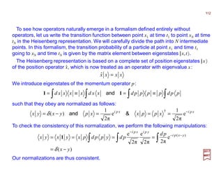
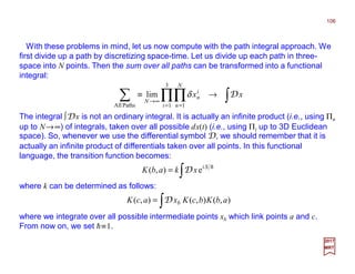
113. Our task is now to rewrite the functional integration over p at an intermediate point
along the path in terms of an operator expression defined in the Heisenberg picture. We
will use the fact that the transition element between two neighboring points can be
written as:
113
2017
MRT
11221
)(
2 ,,e 12
txtxxx ttHi
=−−
Let us take a specific value of x~(x1 −x2)δ t and dp that appears within the functional
integral and carefully rewrite the integral over dp and its integrand as follows:
⋅⋅⋅⋅
1122
1
),(
212
),(
12
),(
),()(),()],([
,,
eee
e
π2
eeee
π2
e
π2
1221
txtx
xxxxxppdpx
pdpdpd
txHitxHitxHi
xpipxitxHixxpitpxHitpxHxpi
xxx
x
=
===
==
∂−∂−∂−
−−∂−−−−−−
∫
∫∫∫
δδδ
δδδ&
xpitpxHixpitxHixpixpi
x
x
pi ⋅−⋅∂−⋅⋅
==∂ eeeeee ),(),( δδ
and
We have now made the transition between a Lagrangian defined in terms of x and x and
a Hamiltonian defined in terms of x and its derivative ∂x. The transition was made
possible because the derivative of the exponential brings down a p:
⋅⋅⋅⋅
In the path integral formalism, this is the origin of the transition between c-numbers
and q-number operators; that is, the insertion of intermediate states defined in p
space allows us to replace the p variable with a ∂x operator. Thus, we have made the
transition between H(x,p)↔H(x,∂x) and p↔−i∂/∂ x.

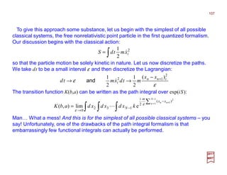
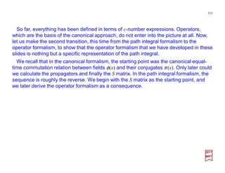
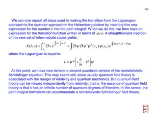
114. In summary, we have now shown that the path integral formalism can express the
propagator K(b,a) in three different ways, in the Lagrangian or Hamiltonian formalism, or
in the operator formalism in the Heisenberg picture. This can be summarized by the
following identity:
114
2017
MRT
∫
∫
∫ ∫
∫
∫
−
−−−−−
=
=
=
=
N
N
t
t
t
t
pxHxptdi
xxLtdi
NNNNNNN
NN
px
x
txtxxdtxtxxdtxtx
txtxNK
1
1
)],([
),(
112222211111
11
e
e
,,,,,,
,,)1,(
&
&
L
DD
D

115. In the first quantized formalism, where the action is a function of x i and not fields, the
path integral formalism gives us an added bonus: It gives us a derivation of the
Schrödinger equation! Usually, introductory courses in quantum mechanics begin by
postulating the Schrödinger wave equation. Certain conventions, such as the
quantization of x and p, seem rather arbitrary. Only later emerges the probabilistic
interpretation. In this Appendix, we reversed this order: we began with Feynman’s
probability-driven rules of quantum mechanics and will now derive the Schrödinger wave
equation as a consequence, this giving a new physical interpretation to that equation.
115
2017
MRT
∫
∞
∞−
= ),(),;,(),( iiiijjijj txtxtxKxdtx ψψ
In the path integral approach, the evolution of a state is given by the transition function
K(b,a). From a classical point of view, this can be viewed as the analogue of Huygen’s
principle, where the evolution of a wave can be determined by assuming that each point
along a wave front emits a new wave front. The integration over all these infinitesimal
wave fronts then gives us the overall evolution of the wave front. Mathematically, this is
given by:
Derivation of the Schrödinger Equation

116. Earlier in this Appendix, we derived, assuming only the Lagrangian ½mvi
2, an
expression for the nonrelativistic transition function. Now let us calculate how wave
fronts move with this transition function. The time evolution, from t to t+ε, is given by:
116
2017
MRT
∫
∞
∞−
−
=+ ),(e
1
),(
2
)(
2 ty
A
ydtx
yxm
i
ψεψ ε
where A=√(2πiε /m). To perform this integration, let dy be replaced by dη, where η=y −x:
∫
∞
∞−
−
+=+ ),(e),( 21 2
txAdtx mi
ηψηεψ εη
Now Taylor expand the left-hand side in terms of ε, and the right-hand side in terms of η:
∫
∞
∞−
−








+
∂
∂
+
∂
∂
+=
∂
∂
+ L2
2
221
2
1
),(e),(
2
xx
txAd
t
tx mi ψ
η
ψ
ηψη
ψ
εψ εη
The integration over dη is easily performed. The integration over the linear term in η
vanishes because it is linear, and the integration over the higher terms vanish in the limit
ε →0. This gives us:
2
2
2
1
xmt
i
∂
∂
−=
∂
∂ ψψ
This partial differential equation is the Schrödinger wave equation, as desired. It is
straightforward to insert a potential V(x) into the path integral, in which case we
derive the Schrödinger wave equation in a potential, which is the traditional starting
point for quantum mechanics.

117. So far, we have only investigated the path integral formalism in the first quantized
formalism, reproducing known results. The reader may complain that the path integral
formalism is an elaborate, powerful machinery that has only rederived simple results.
However, when we make the transition to the second quantized formalism, we will find
that the path integral approach is the preferred formalism for quantum field theory.
117
2017
MRT
∫= iiiii txxdtx ,,1
We saw earlier that the integration over all intermediate points along a path was
enforced by inserting the number 1 at each intermediate point:
From First to Second Quantization
The transition to field theory is made by introducing yet another expression for the
number 1, this time based on an integration over an infinite number of degrees of
freedom. We will use the familiar Gaussian integration:
∫∏=
−∑ =
=
n
l
x
jilnji
n
k k
xxxd
1
2
1
2
e
π
2
δ

118. Now let us replace the variable xi with a function ψ (x), which is temporarily viewed as
a discretized number ψx, where x is now seen as an infinite discrete index. The transition
from finite degrees of freedom to infinite degrees of freedom is then made by inserting
the following expression for 1 into the path integral:
118
2017
MRT
∫
∑−
z zz
yxyx yx
ψψ
ψψψδ
*
e~ **
, DD
where:
∏=
z
zdψψD
Written in terms of functions ψ (x) rather than discretized variables ψz, we now have:
∫ ∫−
=−
2
)(**
e)()()(
xx
yxyx
ψ
ψψψψδ
D
DD
These expressions can also be rewritten in terms of bra and ket vectors as follows:
xxxx ψψψψ == )()( *
and
This allows us to write:
yxyxyxyx
zxzzzx
1===− ∫∫ ∫∫ −−
ψψψψψψδ
ψψψψ DD
DD ee)()()( 2)()(*2
*
So, written in this language, the number 1 now becomes:
∫
−
= ψψψ
ψψ
e2
D1

119. We can now repeat all steps used in making the transition from the Lagrangian
approach to the operator approach in the Heisenberg picture by inserting this new
expression for the number 1 into the path integral. When we do this, we then have an
expression for the transition function written in terms of ψ (x). A straightforward insertion
of this new set of intermediate states yields:
119
2017
MRT
ψψ 





−
∂
∂
= H
t
iL *
where the Lagrangian is equal to:
∫∫ ∫∫ −∂
==
ψψ
ψψψψ
)*(**2
1
e)()(e),(
2
Hitdi
ba
x
x
xmtdi tb
a
i
xxxabK DDD
&
At this point, we have now derived a second quantized version of the nonrelativistic
Schrödinger equation. This may seem odd, since usually quantum field theory is
associated with the merger of relativity and quantum mechanics. But quantum field
theory can be viewed independently from relativity; that is, the essence of quantum field
theory is that it has an infinite number of quantum degrees of freedom. In this sense, the
path integral formalism can accommodate a nonrelativistic Schrödinger field theory.

120. Next, we would like to compute the familiar expressions found in these the previous
content of these slides in terms of the path integral approach. We are notably talking
about Wick’s theorem which, in simple form, is the average (i.e., expectation value) of
time ordered field products (i.e., using the operator T[…]):
120
2017
MRT
)(0)]()([0 yxiyxT F −∆=φφ
This was obtained in the Propagator Theory chapter using the canonical formalism. So,
first, we define the average 〈Y〉 of the expression Y by inserting it into the integral:
∫
∑ =
−
≡ YXNY
n
ji jjii xDx
1, 2
1
eD
Our goal is to find an expression for 〈Y〉, and later make the transition to an infinite
number of degrees of freedom (n →∞). To find an expression for this average, we will
find it convenient to introduce an intermediate stage in the calculation. We define the
generating functional as follows:
∫∏
∑∑ ==
+−
=
≡
n
i ii
n
ji jjii xJxDxn
i
ixdJDI 11, 2
1
1
e],[
where we fix the normalization constant N by setting:
1
]0,[ −
= NDI
Generating Functionals
The square brackets indicate the fact that I is a functional of the functions D and J
(i.e., it gives us a number for each function).

121. To find an expression for I[D,J], we first make the similarity transformation:
121
2017
MRT
jjii xSx =′
such that S diagonalizes the matrix D. We are then left with the eigenvalues of the matrix
D in the integral. The integration separates into a product of independent integrations
over x′i. We then perform each integration separately, giving us the square root of the
eigenvalues of the D matrix. The product of the eigenvalues, however, is equal to the
determinant of the D matrix, giving us the final result:
∑ =
−
−
−
=
n
ki kkii JDJ
ji
n
DJDI 1,
1
][
2
1
212
e)(det)π2(],[

122. Our goal now is to evaluate the average of an arbitrary product x1x2 …xn:
122
2017
MRT
jiji Dxx ][ 1−
=
This expression, for an odd number of xs, vanishes. However, for two xs, we have:
∫∏=
−∑ =
≡
n
i
xDx
nin
n
ji jjii
xxxxdNxxx
1
2
1
2121
1,
eLL
where the normalization constant N can be fixed via:
2121
)(det)π2(]0,[ −−
== ji
n
DNDI
We can also take repeated derivatives of I[D,J] with respect to J, and then set J equal to
zero. Each time we take the derivative ∂/∂Ji, we bring down a factor of xi into the integral:
∑∏ −
−−
= =
=
∂
∂
=
Pairings
11
1 0
21 121
][][
],[
nn kkkk
n
i Ji
n DD
J
JDI
xxx LL
and for four xs, we have:
kjliljkilkjilkji DDDDDDxxxx ][][][][][][ 111111 −−−−−−
++=
Not surprisingly, if we analyze the way in which these indices are paired off, we see
Wick’s theorem beginning to emerge. The point here is that Wick’s theorem, which
was based on arguments concerning normal ordering of operators, is now emerging
from entirely c-number integrations.

123. The transition to quantum field theory, as before, is now made by making the transition
from a finite number of variables xi to an infinite number of variables φ(x). As before, we
are interested in evaluating the transition probability between a field at point x and a field
at point y:
123
2017
MRT
∫ ∫ +
≡
)]()()([4
e][
xxJxxdi
NJZ
φ
φ
L
D
To evaluate this integral, we will find it convenient, as before, to introduce the (Wick
rotated) generating functional:
∫
Si
yx e)()( φφφD
where:
∏≡
x
xd )(φφD
and:
∫ ∫≡− )(1
4
e
xxdi
N
L
φD
where:
∫= )(4
φLxdS
with φ =φ(x).

124. As an example, we will perform this integration for a Klein-Gordon field where we will
repeat the steps we used for the simpler theory based on a finite number of degrees of
freedom. We first make a shift of variables:
124
2017
MRT
)()()( cl xxx φφφ +→
where φcl satisfies the Klein-Gordon equation with a source term, J. We recall that the
Feynman propagator is defined via:
)()()( 42
yxyxm Fx −−=−∆+∂∂ δµ
µ
A classical solution can the be defined via:
∫ −∆−= )()()( 4
cl yJyxydx Fφ
which satisfies:
)()( cl
2
xJm =+∂∂ φµ
µ

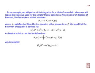
125. We can now perform the integral by performing a Gaussian integration:
125
2017
MRT
where:
∫ −∆−
=
)()()(
2
44
e][
yJyxxJydxd
i
F
JZ
∫ ∫=+∂=− )(21221
4
e)][det(
xxdi
mN
L
φµ D
Using the fact that [δ/δ J(x)] J( y)=δ 4(x−y) we find that the transition function is given by:
0
][
)()(
)( =
=−∆− JF JZ
yJxJ
yxi
δ
δ
δ
δ
The average of several fields taken at point xi is now given as follows:
021
2121
)()()(
][
0)]()()([0),,,(
=
==∆
Jn
n
n
n
nF
xJxJxJ
JZ
xxxTixxx
δδδ
δ
φφφ
L
LL
By explicit differentiation, we can take the derivatives for four fields and find:
In this way, we have derived Wick’s theorem starting with purely c-number
expressions.
)()()()(
)()(][
)(
32414231
43210
1
xxxxxxxx
xxxxJZ
xJ
FFFF
FFJ
n
i i
−∆−∆+−∆−∆+
−∆−∆=








− =
=
∏δ
δ

126. Z[J] can also be written as a power expansion in J. If we power expand the generating
functional, then we have:
126
2017
MRT
∑ ∫ ∫
∞
=
=
0
1
)(
1
4
1
4
),,()()(
!
1
][
n
n
n
nn xxZxJxJxdxd
n
JZ LLLL
where:
0)]()([0][
)()(
),,( 10
1
1
)(
n
n
J
n
n
n
n
xxTiJZ
xJxJ
xxZ φφ
δδ
δ
L
L
L == =
In this way now, the path integral method can derive all the expressions found earlier in
the canonical formalism.

127. The functional techniques allows us to formulate QED based on the Schwinger-Dyson
integral equation. This equation, when power expanded, yields the standard perturbation
theory. But since we do not necessarily have to power expand these equations, these
integral equations also apply to bound-state and nonperturbative problems.
127
2017
MRT
0≡∫ φδ
δ
φD
The Schwinger-Dyson equation is based on the deceptively simple observation that
the integral of a derivative is zero:
Schwinger-Dyson Equations
where:
∏≡
x
xd )(φφD
Although this statement appears trivial from the point of view of functional analysis, it
yields highly nontrivial relations among generating functionals in quantum field theory.

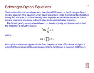
128. In particular, let us act on the generating functional Z[J] for a scalar field theory:
128
2017
MRT
This can be rewritten as:
0e
)()(4
=∫ ∫+ xxJxdiSi φ
φδ
δ
φD
where S =S(φ) is the action (e.g., based on L =½(∂µ φ)2 −V(φ)). The functional derivative
of the source term simply pulls down a factor of J. We simply get:
0e)(
)()(4
=





+
∂
∂
∫ ∫+ xxJxdiSi
xJi
S
i
φ
φ
φD
0][)(
)(
=








+





−
∂
∂
JZxJ
xJ
i
S
δ
δ
φ
This is the Schwinger-Dyson relation, which is independent of perturbation theory. As
this point, we can take any number of derivatives of this equation with respect to the
fields and obtain a large number of integral equations involving various Green functions.
Or, we can power expand this equation and reproduce the known perturbation theory.
For QED, the generalization of the Schwinger-Dyson relation reads:
0],,[,, =








+







−− ηη
ηδ
δ
ηδ
δ
δ
δ
δ
δ
µ
νµ
JZJii
J
iS
A

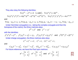
129. Independent of any representation, the Dirac matrices obey a number of identities that
follow from the definition:
where (N.B., the specific choice of representations for these matrices will be given very
soon):
129
2017
MRT
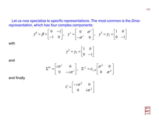
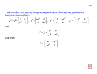
Appendix III: Dirac Matrices
νµµννµνµ
ηγγγγγγ 2},{ =+=
1
!4
2
5
3210
5
50
=−===== γγγγγεγγγγγγαβγβγ σρνµ
σρνµ and,,
i
iii
and ηµν =diag(+1,−1,−1,−1). Also:
σρ
σρνµνµµννµνµνµ
εγγγγγγγ Σ=Σ−==Σ
2
)(
2
],[
2
5 iii
and
Note as well:
µ
µ
νµ
νµ γaabaibaba =/Σ−⋅=// with
and the various gamma matrices identities:
νρσ
µ
σρνµρν
µ
ρνµν
µ
νµ
µ
µ
γγγγγγγγηγγγγγγγγγγ 2424 −==−== ,,,
and
)(2 τνσρσρντ
µ
τσρνµ
γγγγγγγγγγγγγγ −=
and also:
ρνσ
µ
σρνµ
µ
ρνµ
γγγγγγ Σ=Σ=Σ 20 and

130. They also obey the following identities:
Under Hermitian conjugation (i.e., taking the complex conjugate and then the
transpose of the matrix), the Dirac matrices obey:
130
2017
MRT
( )
σρνµσρνµρνσµσνρµσρνµσρνµ
νµνµµµ
εγγγγγηηηηηηγγγγ
ηγγγγ
i
nn
4)(Tr)(4)(Tr
4)(Tr0)(Tr
5
1
−=+−=
==
,
,,oddL
)(Tr)(Tr)(Tr)(Tr 12221242312532121 −//++///⋅−///⋅=// nnnnn aaaaaaaaaaaaaaaa LLLLLL
and
ii
γγγγ −== †0†0
and
with the identities:
Under charge conjugation, the Dirac matrices also obey:
†00†
5
0
5
0
5
†
5
0
5
0†00
)()( νµνµµµµµ
γγγγγγγγγγγγγγγγγ Σ=Σ=−=−== and,,
,,,T
11 ††2†
===−== CCCCCCC
TTTT
,,, )( 5
1
5
1
5
1
5
1
µµνµνµµµ γγγγγγγγ =Σ−=Σ=−= −−−−
CCCCCCCC
and
For future reference, we have the Pauli spin matrices:






−
=




 −
=





=
10
01
0
0
01
10 321
σσσ and,
i
i

131. Let us now specialize to specific representations. The most common is the Dirac
representation, which has four complex components:
with
131
2017
MRT






−
==








−
=





−
−
==
10
01
0
0
01
10
5
50
γγ
σ
σ
γβγ ,, i
i
i








=Σ








−
=Σ k
k
kji
ji
i
i
i
i
i
σ
σ
ε
σ
σ
0
0
0
00
,
and finally







−
= 2
2
0
0
σ
σ
i
i
C






−
==
10
01
5
5
γγ
and

132. We can also take a purely imaginary representation of the spinors, given by the
Majorana representation:
132
2017
MRT
and








−
== 2
2
5
5
0
0
σ
σ
γγ
and finally








−
−
=
0
0
2
2
σ
σ
iC








−
−
=







 −
=








=








== 1
1
3
2
2
2
3
3
1
2
2
0
0
0
0
0
0
0
0
0
σ
σ
γ
σ
σ
γ
σ
σ
γ
σ
σ
βγ
i
i
i
i
,,,

133. We define conjugate spinors by:
On-shell, the spinors u and v represent the electron (with negative charge −e) and
positron (i.e., a positive charge electron) wave functions, respectively. They obey:
133
2017
MRT
The spinors u and v are normalized as follows:
0†0†0†
γγγψψ vvuu === and,
0))((0))((0)()(0)()( =+/=−/=+/=−/ mppvmppupvmppump and,,
1),()(1),(),( −== spvpvspuspu and
These spinors also obey certain completeness relations:
,βαβαβα δ=−∑s
spvspvspuspu )],(),(),(),([
βα
βα
βα
βα
γγ





 /+/−
−=




 /++/=
2
1
2
),(),(
2
1
2
),(),( 55 s
m
pm
spvspv
s
m
mp
spuspu and
as well as
If we sum over the helicity s (sometimeslabeled as σ) we have two projection operators:
These are projection operators, and hence they satisfy:
βα
βαβα
βα
βαβα 




 +/−
=−=Λ




 +/==Λ ∑∑ ±
−
±
+
m
mp
spvspvp
m
mp
spuspup
ss
2
),(),()(
2
),(),()( ][&][
102
=Λ+Λ=ΛΛΛ=Λ −+−+±± and,

134. References / Study Guide
2017
MRT
134
J.J. Sakurai, Advanced Quantum Mechanics, Addison-Wesley, 1967.
University of California at Los Angeles
The tenth printing [mine] of this renowned textbook confirms its widely-regarded status as a classic. The book presents the major
advances in the fundamentals of quantum physics from 1927 to the present day [1967]. No familiarity with relativistic quantum
mechanics of quantum field theory is presupposed, but the reader is assumed to be familiar with non-relativistic quantum mechanics,
classical electrodynamics, and classical mechanics. The author’s clear presentation focuses on key concepts, giving attention to
experimental work in the field.
M. Kaku, Quantum Field Theory – A Modern Introduction, Oxford University Press, 1993
City College of the CUNY
The rise of quantum electrodynamics (QED) made possible a number of excellent textbooks on quantum field theory in the 1960s.
However, the rise of quantum chromodynamics (QCD) and the Standard Model has made it urgent to have a fully modern textbook
for the 1990s and beyond. Building on the foundation of QED, Quantum Field Theory: A Modern Introduction presents a clear and
comprehensive discussion of the gauge revolution and the theoretical and experimental evidence which makes the Standard Model
the leading theory of subatomic phenomena. The book is divided into three parts: Part I, Fields and Renormalization, lays a solid
foundation by presenting canonical quantization, Feynman rules and scattering matrices, and renormalization theory. Part II, Gauge
Theory and the Standard Model, focuses on the Standard Model and discusses path integrals, gauge theory, spontaneous symmetry
breaking, the renormalization group, and BPHZ quantization. Part III, Non-perturbative Methods and Unification, discusses more
advanced methods which now form an essential part of field theory, such as critical phenomena, lattice gauge theory, instantons,
supersymmetry, quantum gravity, supergravity, and superstrings.
T. Ohlsson, Relativistic Quantum Physics, Cambridge University Press, 2011.
Royal Institute of Technology (KTH), Sweden
Quantum physics and special relativity theory were two of the greatest breakthroughs in physics during the twentieth century and
contributed to paradigm shifts in physics. This book combines these two discoveries to provide a complete description of the
fundamentals of relativistic quantum physics, guiding the reader effortlessly from relativistic quantum mechanics to basic quantum
field theory. The book gives a thorough and detailed treatment of the subject, beginning with the classification of particles, the Klein-
Gordon equation and the Dirac equation. It then moves on to the canonical quantization procedure of the Klein-Gordon, Dirac and
electromagnetic fields. Classical Yang-Mills theory, the LSZ formalism, perturbation theory, elementary processes in QED are
introduced, and regularization, renormalization and radiative corrections are explored. With exercises scattered through the text and
problems at the end of most chapters, the book is ideal for advanced undergraduate and graduate students in theoretical physics.
T. Banks, Modern Quantum Field Theory: A Concise Introduction, Cambridge University Press, 2008.
University of California, Santa Cruz, and Rutgers University
This comprehensive and progressive new text presents a variety of topics that are only briefly touched on in other books; this text
provides a thorough introduction to the techniques of quantum field theory, which is the theoretical framework for constructing
quantum mechanical models of field-like systems or, equivalently, of many-body systems. […] The Standard Model of particle
physics is also discussed in detail. […] Ideal for graduate students in high-energy physics and condensed matter physics […]

135. Three quantum paths from A to B given by the functional (i.e., a function of functions):
∫= t
tABLtdABS 0 )]([][
)]([)(
2
1
)]([)]([)]([
2
tABVtAB
t
m
tABVtABTtABL
−





∂
∂
=
−=
with the Lagrangian given by (i.e., the
difference between kinetic T and
potential V energies):
t
r
A
B
∫=
B
A
ABS
i
AB
ABZ
][
e)( hD
where the action is defined as being:
For a free particle of mass m, V =0.
The potential V can be represented as a
scalar field in some localized region of
space-time and once the particle ‘feels’
its effect, the Lagrangian take account
of it – it will ‘influence’ the path of the
particle. When h→0, only a single path
in space-time becomes discernible!
2017
MRT
∫
∫ −
=
B
A
Vdtdmtd
i
AB
t
ABdtdtZ 0
2
)}(]/[½{
e)(]/),([
rr
rr hD
Generating functional:

136. so
2017
MRT
Feynman’s path integral solution over the interval (x1,t1) to (xN,tN) is:
where ∆t =(tN −t1)/(N −1) and ∫D[x(t)] is an infinite-dimensional integral operator.