Download to read offline
![Introduction
Books
W. Pauli, “Die Allgemeinen Principien der Wellenmechanik”; Handbuch der Physik, 2 ed., Vol. 24,
Part 1; Edwards reprint, Ann Arbor 1947. (In German) [1]
W. Heitler, Quantum Theory of Radiation, 2nd Edition, Oxford. 3rd edition just published. [2]
G. Wentzel, Introduction to the Quantum Theory of Wave-Fields, Interscience, N.Y. 1949 [3]
I shall not expect you to have read any of these, but I shall refer to them as we go along. The later part
of the course will be new stuff, taken from papers of Feynman and Schwinger mainly. [4], [5], [6], [7], [8]
Subject Matter
You have had a complete course in non-relativistic quantum theory. I assume this known. All the general
principles of the NR theory are valid and true under all circumstances, in particular also when the system
happens to be relativistic. What you have learned is therefore still good.
You have had a course in classical mechanics and electrodynamics including special relativity. You know
what is meant by a system being relativistic; the equations of motion are formally invariant under Lorentz
transformations. General relativity we shall not touch.
This course will be concerned with the development of a Lorentz–invariant Quantum theory. That is not
a general dynamical method like the NR quantum theory, applicable to all systems. We cannot yet devise
a general method of that kind, and it is probably impossible. Instead we have to find out what are the
possible systems, the particular equations of motion, which can be handled by the NR quantum dynamics
and which are at the same time Lorentz–invariant.
In the NR theory it was found that almost any classical system could be handled, i.e.quantized. Now
on the contrary we find there are very few possibilities for a relativistic quantized system. This is a most
important fact. It means that starting only from the principles of relativity and quantization, it is mathe-
matically possible only for very special types of objects to exist. So one can predict mathematically some
important things about the real world. The most striking examples of this are:
(i) Dirac from a study of the electron predicted the positron, which was later discovered [9].
(ii) Yukawa from a study of nuclear forces predicted the meson, which was later discovered [10].
These two examples are special cases of the general principle, which is the basic success of the relativistic
quantum theory, that A Relativistic Quantum Theory of a Finite Number of Particles is Impossible. A RQ
theory necessarily contains these features: an indefinite number of particles of one or more types, particles
of each type being identical and indistinguishable from each other, possibility of creation and annihilation
of particles. Thus the two principles of relativity and quantum theory when combined lead to a world built
up out of various types of elementary particles, and so make us feel quite confident that we are on the right
way to an understanding of the real world. In addition, various detailed properties of the observed particles
1](https://image.slidesharecdn.com/advancedquantummechanics-230806151100-7e1e8919/75/Advanced-Quantum-Mechanics-7-2048.jpg)
![INTRODUCTION 2
are necessary consequences of the general theory. These are for example:
(i) Magnetic moment of Electron (Dirac) [9].
(ii) Relation between spin and statistics (Pauli) [11].
Detailed Program
We shall not develop straightaway a correct theory including many particles. Instead we follow the historical
development. We try to make a relativistic quantum theory of one particle, find out how far we can go
and where we get into trouble. Then we shall see how to change the theory and get over the trouble by
introducing many particles. Incidentally, the one–particle theories are quite useful, being correct to a good
approximation in many situations where creation of new particles does not occur, and where something
better than a NR approximation is needed. An example is the Dirac theory of the H atom.1
The NR theory gave levels correctly but no fine-structure. (Accuracy of one part in 10,000). The Dirac
one-particle theory gives all the main features of the fine-structure correctly, number of components and
separations good to 10% but not better. (Accuracy one part in 100,000).
The Dirac many-particle theory gives the fine-structure separations (Lamb experiment) correctly to
about one part in 10,000. (Overall accuracy 1 in 108
.)
Probably to get accuracy better than 1 in 108
even the DMP theory is not enough and one will need
to take all kinds of meson effects into account which are not yet treated properly. Experiments are so far
only good to about 1 in 108
.
In this course I will go through the one-particle theories first in detail. Then I will talk about their
breaking down. At that point I will make a fresh start and discuss how one can make a relativistic quantum
theory in general, using the new methods of Feynman and Schwinger. From this we shall be led to the
many-particle theories. I will talk about the general features of these theories. Then I will take the special
example of quantum electrodynamics and get as far as I can with it before the end of the course.
One-Particle Theories
Take the simplest case, one particle with no forces. Then the NR wave-mechanics tells you to take the
equation E =
1
2m
p2
of classical mechanics, and write
E → i~
∂
∂t
px → −i~
∂
∂x
(1)
to get the wave-equation2
i~
∂
∂t
ψ = −
~2
2m
∂2
∂x2
+
∂2
∂y2
+
∂2
∂z2
ψ = −
~2
2m
∇2
ψ (2)
satisfied by the wave-function ψ.
To give a physical meaning to ψ, we state that ρ = ψ∗
ψ is the probability of finding the particle at the
point x y z at time t. And the probability is conserved because3
∂ρ
∂t
+ ∇ ·~
= 0 (3)
where
~
=
~
2mi
(ψ∗
∇ψ − ψ∇ψ∗
) (4)
where ψ∗
is the complex conjugate of ψ.
Now do this relativistically. We have classically
E2
= m2
c4
+ c2
p2
(5)](https://image.slidesharecdn.com/advancedquantummechanics-230806151100-7e1e8919/75/Advanced-Quantum-Mechanics-8-2048.jpg)
![INTRODUCTION 3
which gives the wave equation
1
c2
∂2
∂t2
ψ = ∇2
ψ −
m2
c2
~2
ψ (6)
This is an historic equation, the Klein-Gordon equation. Schrödinger already in 1926 tried to make a RQ
theory out of it. But he failed, and many other people too, until Pauli and Weisskopf gave the many-particle
theory in 1934 [12]. Why?
Because in order to interpret the wave-function as a probability we must have a continuity equation.
This can only be got out of the wave-equation if we take ~
as before, and
ρ =
i~
2mc2
ψ∗ ∂ψ
∂t
−
∂ψ∗
∂t
ψ
(7)
But now since the equation is 2nd
order, ψ and
∂ψ
∂t
are arbitrary. Hence ρ need not be positive. We have
Negative Probabilities. This defeated all attempts to make a sensible one-particle theory.
The theory can be carried through quite easily, if we make ψ describe an assembly of particles of
both positive and negative charge, and ρ is the net charge density at any point. This is what Pauli and
Weisskopf did, and the theory you get is correct for π-mesons, the mesons which are made in the synchrotron
downstairs. I will talk about it later.](https://image.slidesharecdn.com/advancedquantummechanics-230806151100-7e1e8919/75/Advanced-Quantum-Mechanics-9-2048.jpg)
![The Dirac Theory
The Form of the Dirac Equation
Historically before the RQ theory came the one-particle theory of Dirac. This was so successful in dealing
with the electron, that it was for many years the only respectable RQ theory in existence. And its difficulties
are a lot less immediate than the difficulties of the one-particle KG theory.
Dirac said, suppose the particle can exist in several distinct states with the same momentum (different
orientations of spin.) Then the wave-function ψ satisfying (6) must have several components; it is not a
scalar but a set of numbers each giving the prob. amplitude to find the particle at a given place and in a
given substate. So we write for ψ a column matrix
ψ =
ψ1
ψ2
·
·
·
for the components ψα ; α = 1, 2, . . .
Dirac assumed that the probability density at any point is still given by
ρ =
X
α
ψ∗
αψα (8)
which we write
ρ = ψ∗
ψ
as in the NR theory. Here ψ∗
is a row matrix
[ψ∗
1, ψ∗
2, . . . ]
We must have (3) still satisfied. So ψ must satisfy a wave-equation of First Order in t. But since the
equations are relativistic, the equation has to be also of 1st
order in x y z. Thus the most general possible
wave-equation is
1
c
∂ψ
∂t
+
3
X
1
αk ∂ψ
∂xk
+ i
mc
~
β ψ = 0 (9)
where x1 x2 x3 are written for x y z and α1
α2
α3
β are square matrices whose elements are numbers. The
conjugate of (9) gives
1
c
∂ψ∗
∂t
+
3
X
1
∂ψ∗
∂xk
αk∗
− i
mc
~
ψ∗
β∗
= 0 (10)
where αk∗
and β∗
are Hermitian conjugates.
Now to get (3) out of (8), (9) and (10) we must have αk∗
= αk
, β∗
= β so αk
and β are Hermitian; and
jk = c ψ∗
αk
ψ
(11)
4](https://image.slidesharecdn.com/advancedquantummechanics-230806151100-7e1e8919/75/Advanced-Quantum-Mechanics-10-2048.jpg)
![THE DIRAC THEORY 9
γ1 =
0 0 −i
−i 0
0 i
i 0 0
; γ2 =
0 0 −1
1 0
0 1
−1 0 0
; γ3 =
0 −i 0
0 i
i 0
0 −i 0
; γ4 =
1 0
0 1 0
0 −1 0
0 −1
are a 4-vector. They are all Hermitian and satisfy
γµγν + γνγµ = 2δµν (33)
The Dirac equation and its conjugate may now be written
4
X
1
γµ
∂ψ
∂xµ
+
mc
~
ψ = 0
4
X
1
∂ψ
∂xµ
γµ −
mc
~
ψ = 0 (34)
with
ψ = ψ∗
β and (35)
sµ = i ψ γµ ψ
=
1
c
~
, iρ
(36)
These notations are much the most convenient for calculations.
Conservation Laws. Existence of Spin.
The Hamiltonian in this theory is6
i~
∂ψ
∂t
= Hψ (37)
H = −i~c
3
X
1
αk ∂
∂xk
+ mc2
β = −i~c α · ∇ + mc2
β (38)
This commutes with the momentum p = −i~∇. So the momentum p is a constant of motion.
However the angular momentum operator
L = r × p = −i~r × ∇ (39)
is not a constant. For
[H, L] = −~2
c α × ∇ (40)
But
[H, σ] = −i~c ∇ · [α, σ] where σ = (σ1, σ2, σ3)
while
α1
, σ1
= 0,
α1
, σ2
= 2iα3
,
α1
, σ3
= −2iα2
, etc.
So
[H, σ3] = 2~c α1
∇2 − α2
∇1
and thus
[H, σ] = 2~c α × ∇ (41)
Thus
L + 1
2 ~σ = ~J (42)](https://image.slidesharecdn.com/advancedquantummechanics-230806151100-7e1e8919/75/Advanced-Quantum-Mechanics-15-2048.jpg)
![THE DIRAC THEORY 10
is a constant, the total angular momentum, because by (40), (41) and (42)
[H, J] = 0
L is the orbital a. m. and 1
2 ~σ the spin a. m. This agrees with the N. R. theory. But in that theory the
spin and L of a free particle were separately constant. This is no longer the case.
When a central force potential V (r) is added to H, the operator J still is constant.
Elementary Solutions
For a particle with a particular momentum p and energy E, the wave function will be
ψ(x, t) = u exp
i
p · x
~
− i
Et
~
(43)
where u is a constant spinor. The Dirac equation then becomes an equation for u only
Eu = c α · p + mc2
β
u (44)
We write now
p+ = p1 + ip2 p− = p1 − ip2 (45)
Then (44) written out in full becomes
E − mc2
u1 = c (p3u3 + p−u4)
E − mc2
u2 = c (p+u3 − p3u4)
(46)
E + mc2
u3 = c (p3u1 + p−u2)
E + mc2
u4 = c (p+u1 − p3u2)
These 4 equations determine u3 and u4 given u1 and u2, or vice-versa. And either u1 and u2, or u3 and u4,
can be chosen arbitrarily provided that7
E2
= m2
c4
+ c2
p2
(47)
Thus given p and E = +
p
m2c4 + c2p2, there are two independent solutions of (46); these are, in non-
normalized form:
1
0
c p3
E + mc2
c p+
E + mc2
0
1
c p−
E + mc2
−c p3
E + mc2
(48)
This gives the two spin-states of an electron with given momentum, as required physically.
But there are also solutions with E = −
p
m2c4 + c2p2. In fact again two independent solutions, making
4 altogether. These are the famous negative energy states. Why cannot we simply agree to ignore these
states, say they are physically absent? Because when fields are present the theory gives transitions from
positive to negative states. e.g.H atom should decay to negative state in 10−10
secs. or less.
Certainly negative energy particles are not allowed physically. They can for example never be stopped
by matter at rest, with every collision they move faster and faster. So Dirac was driven to](https://image.slidesharecdn.com/advancedquantummechanics-230806151100-7e1e8919/75/Advanced-Quantum-Mechanics-16-2048.jpg)
![THE DIRAC THEORY 13
since by (57), we have ψγµ = ψ∗
βγµ = (Cφ+
)
T
βγµ = φT
CT
βγµ; the wave function φ = Cψ+
of a positron
satisfies by (65)
X
∂
∂xµ
−
ie
~c
Aµ
γT
µ βCφ −
mc
~
βCφ = 0 (67)
Multiplying by Cβ this gives
X
∂
∂xµ
−
ie
~c
Aµ
γµφ +
mc
~
φ = 0 (68)
This is exactly the Dirac equation for a particle of positive charge (+e). We have used
CβγT
µ βC = −γµ, (69)
which follows from (15), (32), and (55).
The Hydrogen Atom
This is the one problem which it is possible to treat very accurately using the one-electron Dirac theory.
The problem is to find the eigenstates of the equation
Eψ = Hψ
H = −i~c α · ∇ + mc2
β −
e2
r
(70)
As in the NR theory, we have as quantum numbers in addition to E itself the quantities
jz = −i [r × ∇]3 + 1
2 σ3 (71)
j(j + 1) = J2
=
−i (r × ∇) + 1
2 σ
2
(72)
where jz and j are now half-odd integers by the ordinary theory of angular momenta. These quantum
numbers are not enough to fix the state, because each value of j may correspond to two NR states with
ℓ = j ± 1
2 . Therefore we need an additional operator which commutes with H, which will distinguish
between states with σ parallel or antiparallel to J. The obvious choice is
Q = σ · J
But [H, σ] is non-zero and rather complicated. So it is better to try
Q = βσ · J (73)
which is the same in the NR limit.
Then we have
[H, Q] = [H, βσ · J] = [H, βσ] · J + βσ · [H, J]
But [H, J] = 0; furthermore, since
αk
βσℓ = βσℓαk
k 6= ℓ and αk
βσk = −βσkαk
we get
[H, βσ] = −i~c {(α · ∇) βσ − βσ (α · ∇)} = −2i~c
3
X
k=1
αk
σk β ∇k
Therefore
[H, βσ] · J = −2~c
3
X
k=1
αk
σk β ∇k (r × ∇)k − i~c (α · ∇) β = −i~c (α · ∇) β =
H, 1
2 β](https://image.slidesharecdn.com/advancedquantummechanics-230806151100-7e1e8919/75/Advanced-Quantum-Mechanics-19-2048.jpg)
![THE DIRAC THEORY 18
Now in the NR approximation
i~
∂
∂t
= mc2
+ O(1)
(
∂
∂x4
+
ie
~c
A4
2
)
−
m2
c2
~2
=
1
~2c2
(
−i~
∂
∂t
− eΦ
2
− m2
c4
)
=
1
~2c2
−i~
∂
∂t
− eΦ − mc2
−i~
∂
∂t
− eΦ + mc2
=
1
~2c2
−2mc2
+ O(1)
−i~
∂
∂t
− eΦ + mc2
Hence
−i~
∂
∂t
− eΦ + mc2
ψ −
h2
2m
3
X
k=1
(
∂
∂xk
+
ie
~c
Ak
2
)
ψ +
e~
2mc
[σ · H − iα · E] ψ + O
1
mc2
= 0
The NR approximation means dropping the terms O 1/mc2
. Thus the NR Schrödinger equation is
i~
∂ψ
∂t
=
(
mc2
− eΦ −
h2
2m
3
X
k=1
∂
∂xk
+
ie
~c
Ak
2
+
e~
2mc
(σ · H − iα · E)
)
ψ (99)
The term α · E is really relativistic, and should be dropped or treated more exactly. Then we have exactly
the equation of motion of a NR particle with a spin magnetic moment equal to
M = −
e~
2mc
σ (100)
This is one of the greatest triumphs of Dirac, that he got this magnetic moment right out of his general
assumptions without any arbitrariness.
It is confirmed by measurements to about one part in 1000. Note that the most recent experiments
show a definite discrepancy, and agree with the value
M = −
e~
2mc
σ
1 +
e2
2π~c
(101)
calculated by Schwinger using the complete many-particle theory.
Problem 2 Calculate energy values and wave functions of a Dirac particle moving in a homogeneous infinite
magnetic field. Can be done exactly. See F. Sauter, Zeitschrift für Physik 69 (1931) 742.
Solution
Take the field B in the z direction.
A1 = −1
2 By , A2 = 1
2 Bx
The second-order Dirac equation (98) gives for a stationary state of energy ±E
E2
~2c2
−
m2
c2
~2
ψ +
∂
∂x
−
1
2
ieB
~c
y
2
ψ +
∂
∂y
+
1
2
ieB
~c
x
2
ψ +
∂2
∂z2
ψ −
eB
~c
σzψ = 0
Taking a representation with σz diagonal, this splits at once into two states with σz = ±1. Also
Lz = −i~
x
∂
∂y
− y
∂
∂x](https://image.slidesharecdn.com/advancedquantummechanics-230806151100-7e1e8919/75/Advanced-Quantum-Mechanics-24-2048.jpg)


![FIELD THEORY 38
or
i~
d
dt
hφ′ α
1 , t1 φ′ α
2 , t2i = hφ′ α
1 , t1 H (t1) φ′ α
2 , t2i (180)
This is the ordinary Schrödinger equation in Dirac’s notation. It shows that the Schwinger action principle
contains enough information for predicting the future behaviour of a system given initially in a known
quantum state.
C. Operator Form of the Schwinger Principle
Feynman defined operators by giving the formula (175) for their matrix elements between states specified
on two different surfaces. The initial state had to be specified in the past, the final state in the future, the
operator referring to some particular time which is taken as present.
The usual and generally more useful way of defining operators is to specify their matrix elements between
states defined on the same surface. Thus we are interested in a matrix element
hφ′ α
, σ O φ′′ α
, σi (181)
where φ′ α
and φ′′ α
are given sets of eigenvalues and σ is a surface which may be past, present or future in
relation to the field-points to which O refers.
Suppose that a reference surface σo is chosen in the remote past. Let the φα
, σ and L be varied in such
a way that everything on σo remains fixed. For such a variation, (178) gives if we assume that (179) holds
δI(Ω) =
1
c
Z
Ω
δL d4
x +
Z
σ
X
α,µ
παδφα
+
1
c
nµL − φα
µπα
δxµ
dσ (182)
where Ω is the region bounded by σo and σ. Let us now first calculate the variation of (181) arising from
the change in the meaning of the states |φ′ α
, σi and |φ′′ α
, σi. The operator O itself is at this point fixed
and not affected by the variations in φα
, σ and L . Then
hφ′ α
, σ O φ′′ α
, σi =
X
φ′
o
X
φ′′
o
hφ′ α
, σ φ′ α
o , σoi hφ′ α
o , σo O φ′′ α
o , σoi hφ′′ α
o , σo φ′′ α
, σi (183)
therefore, denoting
hφ′ α
, σ O φ′′ α
, σi = hσ′
O σ′′
i etc., we have
δ hσ′
O σ′′
i =
X
′
X
′′
(δ hσ′
σ′
oi) hσ′
o O σ′′
o i hσ′′
o σ′′
i +
X
′
X
′′
hσ′
σ′
oi hσ′
o O σ′′
o i (δ hσ′′
o σ′′
i)
because |φ′ α
o i and |φ′′ α
o i are not changed by the variation, and neither is O. Therefore, using (177) we have
δ hσ′
O σ′′
i =
X
′
X
′′
i
~
hσ′
δIσ−σo O σ′′
i +
X
′
X
′′
i
~
hσ′
O δIσo−σ σ′′
i
where the subscript σ − σo refers to the surface integrals in (178). Since δIσ−σo = −δIσo−σ, we get finally
δ hφ′ α
, σ O φ′′ α
, σi =
i
~
hφ′ α
, σ [ δI(Ω), O ] φ′′ α
, σi (184)
where [ P, R ] = PR − RP. This applies for the case when O is fixed and the states vary.
Now we want to calculate the variation of hφ′ α
, σ O φ′′ α
, σi for the case when the states are fixed, and
O = O (φα
(σ)) changes. This, however, will be the same as for the previous case, except with the opposite
sign, because the variation of the matrix element18
hφ′ α
, σ O φ′′ α
, σi (185)
if both the states and O change simultaneously is zero. Therefore, if we use a representation in which matrix
elements of O are defined between states not subject to variation we get19
i~ δO(σ) = [ δI(Ω), O(σ) ] (186)
This is the Schwinger action principle in operator form. It is related to (177) exactly as the Heisenberg
representation is to the Schrödinger representation in elementary quantum mechanics.](https://image.slidesharecdn.com/advancedquantummechanics-230806151100-7e1e8919/75/Advanced-Quantum-Mechanics-44-2048.jpg)
![FIELD THEORY 39
D. The Canonical Commutation Laws
Taking for σ the space at time t, for O(σ) the operator φα
(r, t) at the space-point r, and δxµ = δL = 0
we have by (182) and (186) for an arbitrary variation δφα
−i~ δφα
(r, t) =
X
β
Z
[ πβ(r′
, t) δφβ
(r′
, t), φα
(r, t) ] d3
r′
(187)
because dσ = −nµ dσµ = −i(−i dx′
1dx′
2dx′
3) = −d3
r′
by (158); the unit vector in the increasing time
direction is i, and this is the outward direction since we choose σo in the past. Hence for every r, r′
[ φα
(r, t), πβ(r′
, t) ] = i~ δαβ δ3
(r − r′
) (188)
Also since the φα
(r) on σ are assumed independent variables,
[ φα
(r, t), φβ
(r′
, t) ] = 0 (189)
So this method gives automatically the correct canonical commutation laws for the fields. There is no need
to prove that the commutation rules are consistent with the field equations, as was necessary in the older
methods.
E. The Heisenberg Equation of Motion for the Operators
Suppose that σ is a flat surface at time t, and that a variation is made by moving the surface through the
small time δt as in B above. But now let O(t) = O(σ) be an operator built up out of the field-operators
φα
on σ. Then by (165) and (186) the change in O(t) produced by the variation is given by
i~ δO(t) = [ − H(t) δt, O(t) ]
That is to say, O(t) satisfies the Heisenberg equation of motion
i~
dO(t)
dt
= [ O(t), H(t) ] (190)
where H(t) is the total Hamiltonian operator.
F. General Covariant Commutation Laws
From (186) we derive at once the general covariant form of the commutation laws discovered by Peierls in
1950 [13]. This covariant form is not easy to reach in the Hamiltonian formalism.
Let two field points z and y be given, and two operators R(z) and Q(y) depending on the field quantities
φα
at z and y. Let a reference surface σo be fixed, past of both z and y. Suppose the quantity,
δR(L ) = ǫ δ4
(x − z) R(z) (191)
is added to the Lagrangian density L (x), where ǫ is an infinitesimal c-number This will make at most
a certain infinitesimal change ǫ δRφα
(x) in the solutions φα
(x) of the field equations. Supposing the new
φα
(x) to be identical with the old one on σo then δRφα
(x) is different from zero only in the future light-cone
of z.
Similarly adding
δQ(L ) = ǫ δ4
(x − y) Q(y) (192)
to L (x) produces at most a change ǫ δQφα
(x) in the φα
(x). Let ǫ δRQ(y) be the change in Q(y) produced
by the addition (191), while ǫ δQR(z) be the change in R(z) produced by (192). Suppose y lies on a surface](https://image.slidesharecdn.com/advancedquantummechanics-230806151100-7e1e8919/75/Advanced-Quantum-Mechanics-45-2048.jpg)
![FIELD THEORY 40
σ lying in the future of z. Then we take Q(y) for O(σ) in (186), and δL given by (191). The δI(Ω) given
by (182) reduces then simply to
δI(Ω) =
1
c
ǫ R(z)
It is assumed that there is no intrinsic change δφα
of φα
or δxµ of σ apart from the change whose effect is
already included in the δL term. Thus (186) gives
[ R(z), Q(y) ] = i~c δRQ(y) (y0 z0)
[ R(z), Q(y) ] = −i~c δQR(z) (z0 y0) (193)
When y and z are separated by a space-like interval, the commutator is zero, because the disturbance R(z)
propagates with a velocity at most c and therefore can affect things only in the future lightcone of z; this
means δRQ(y) = 0 in this case.
Peierls’ formula, valid for any pair of field operators, is
[ R(z), Q(y) ] = i~c {δRQ(y) − δQR(z)} (194)
This is a useful formula for calculating commutators in a covariant way.
G. Anticommuting Fields
There is one type of field theory which can be constructed easily by Schwinger’s action principle, but which
does not come out of Feynman’s picture. Suppose a classical field theory in which a group of field operators
ψα
always occurs in the Lagrangian in bilinear combinations like ψβ
ψα
with the group of field operators
ψ. Examples, the Dirac LD and the quantum electrodynamics LQ.
Then instead of taking every φα
on a given surface σ to commute as in (189), we may take every pair
of ψα
to anticommute, thus20
{ ψα
(r, t), ψβ
(r′
, t) } = 0 { P, R } = PR + RP (195)
The bilinear combination will still commute, like the φα
’s did before. The ψα
commute as before with
any field quantities on σ other than the ψ and ψ. Schwinger then assumes (177) to hold precisely as before,
except that in calculating δI(Ω) according to (178), the variation δψα
anticommutes with all operators ψα
and ψβ
. In these theories it turns out that the momentum πα conjugate to ψα
is just a linear combination
of ψ, because the Lagrangian is only linear in the derivatives of ψ. With the anticommuting fields the field
equations (179) are deduced as before, also the Schrödinger equation (180), the commutation rules being
given by (186) and (187). But now in order to make (187) valid, since δψβ
anticommutes with the ψ and
π operators,21
the canonical commutation law must be written
{ ψα
(r, t), πβ(r′
, t) } = −i~ δαβ δ3
(r − r′
) (196)
The general commutation rule (194) is still valid provided that Q and R are also expressions bilinear in the
ψ and ψ.
The interpretation of the operators, and the justification for the Schwinger principle, in the case of
anticommuting fields, is not clear. But it is clear that the Schwinger principle in this case gives a consistent
and simple formulation of a relativistic quantum field theory. And we may as well take advantage of the
method, even if we do not quite understand its conceptual basis. The resulting theory is mathematically
unambiguous, and gives results in agreement with experiment; that should be good enough.](https://image.slidesharecdn.com/advancedquantummechanics-230806151100-7e1e8919/75/Advanced-Quantum-Mechanics-46-2048.jpg)
![EXAMPLES OF QUANTIZED FIELD THEORIES 42
where DA is the advanced potential of the same source,
DA(x) =
1
4π|r|
δ(x0 + |r|)
Hence we have the the commutation rule (194)
[ Aµ(z), Aλ(y) ] = i~c δλµ [DA(z − y) − DR(z − y)]
= i~c δλµD(z − y) (definition of D) (203)
This invariant D-function satisfies by (200)
2
D(x) = −δ4
(x) − (−δ4
(x)) = 0 (204)
as it must. Also
D(x) =
1
4π|r|
[δ(x0 + |r|) − δ(x0 − |r|)]
= −
1
2π
ǫ(x) δ(x2
) ǫ(x) = sign(x0) (205)
Momentum Representations
We have
δ4
(x) =
1
(2π)4
Z
exp(ik · x) d4
k (206)
where the integral is fourfold, over dk1 dk2 dk3 dk4. Therefore
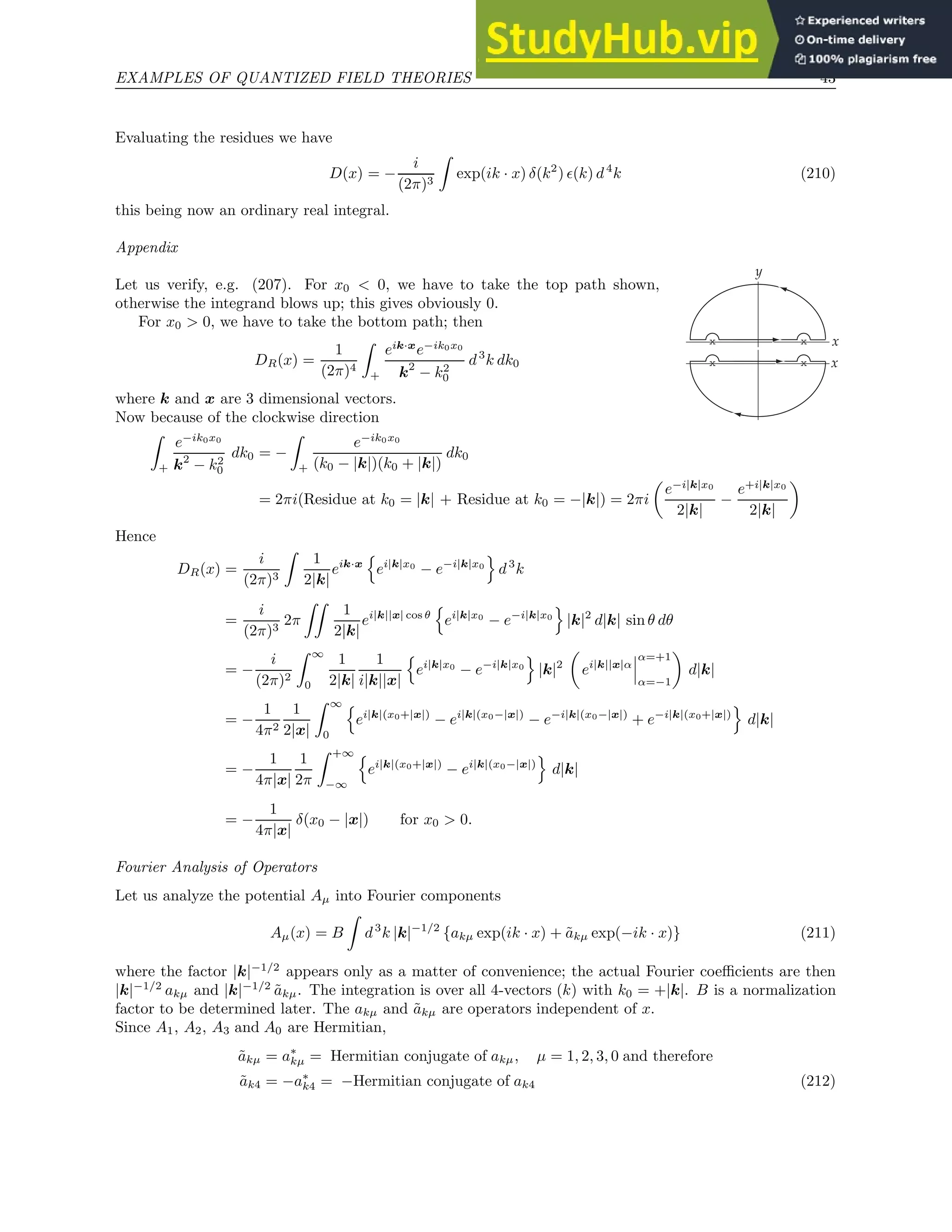
DR(x) =
1
(2π)4
Z
+
exp(ik · x)
1
k2
d4
k (207)
where k2
= |k|2
− k2
0. The integration with respect to k1 k2 k3 is an ordinary real integral. That with
respect to k0 is a contour integral going along the real axis and above the two poles at k0 = ±|k|.
x x
For detailed calculations, see the Appendix below. This gives the correct behaviour of DR being zero for
x0 0. Similarly
DA(x) =
1
(2π)4
Z
−
exp(ik · x)
1
k2
d4
k (208)
with a contour going below both the poles. Therefore
D(x) =
1
(2π)4
Z
s
exp(ik · x)
1
k2
d4
k (209)
with a contour s as shown.
x x
s](https://image.slidesharecdn.com/advancedquantummechanics-230806151100-7e1e8919/75/Advanced-Quantum-Mechanics-48-2048.jpg)
![EXAMPLES OF QUANTIZED FIELD THEORIES 44
Computing the commutator [ Aµ(z), Aλ(y) ] from (211) and comparing the result with (203) in the
momentum representation (210), we have first, since the result is a function of (z − y) only22
[ akµ, ak′λ ] = 0
[ ãkµ, ãk′λ ] = 0 (213)
[ akµ, ãk′λ ] = δ3
(k − k′
) δµλ
And the two results for the commutator agree then precisely if we take
B =
r
~c
16π3
(214)
Emission and Absorption Operators
The operators Aµ(x) obey the Heisenberg equations of motion for operators (190)
i~
∂Aµ
∂t
= [ Aµ, H ] (190a)
Therefore the operator akµ exp(ik · x) has matrix elements between an initial state of energy E1 and a final
state of energy E2, only if
i~(−ick0) = E1 − E2 = ~c|k| (215)
because by (211) and (190a) we have
ψ1 i~(−ick0)akµ ψ2 = ψ1 ~c|k| akµ ψ2 = ψ1 [ aµk, H ] ψ2 = (E1 − E2)ψ1 aµk ψ2 (216)
Now ~c|k| is a constant energy, characteristic of the frequency ω = ck characteristic of the particular Fourier
components of the field. The operator akµ can only operate so as to reduce the energy of a system by a
lump of energy of this size. In the same way, ãkµ will only operate when
E1 − E2 = −~c|k|
to increase the energy by the same amount.
This is the fundamental property of the quantized field operators, that they change the energy of a
system not continuously but in jumps. This shows that our formalism includes correctly the experimentally
known quantum behaviour of radiation.
We call akµ the absorption operator for the field oscillator with propagation vector k and polarization
direction µ. Likewise ãkµ the emission operator.
We have thus 4 directions of polarization for a photon of given momentum. There are not all observed
in electromagnetic radiation. Free radiation can only consist of transverse waves, and has only 2 possible
polarizations. This is because the physically allowable states Ψ are restricted by a supplementary condition
X
µ
∂A
(+)
µ
∂xµ
Ψ = 0 (217)
where A
(+)
µ is the positive frequency part of Aµ, i.e. the part containing the absorption operators. In the
classical theory we have
X
µ
∂Aµ
∂xµ
= 0
the condition imposed in order to simplify the Maxwell equations to the simple form 2
Aµ = 0. In the
quantum theory it was usual to take
X
µ
∂Aµ
∂xµ
Ψ = 0](https://image.slidesharecdn.com/advancedquantummechanics-230806151100-7e1e8919/75/Advanced-Quantum-Mechanics-50-2048.jpg)
![EXAMPLES OF QUANTIZED FIELD THEORIES 46
Then we have at once
hakµak′λio = 0 by (217a) (219a)
hãkµãk′λio = 0 by (217b) (219b)
hãkµak′λio = 0 by (217a,b) (219c)
And by the commutation laws (213) and (219c) we have
hakµãk′λio = h [ akµ, ãk′λ ] io = δ3
(k − k′
) δµλ (220)
The vacuum expectation value hAµ(z) Aλ(y)io is thus just the part of the commutator [ Aµ(z), Aλ(y)]
which contains positive frequencies exp{ik · (z − y)} with k0 0, as one can see using (211), (219) and
(220). Thus25
hAµ(z) Aλ(y)io = i~c δµλ D+
(z − y) (221)
D+
(x) = −
i
(2π)3
Z
k00
exp(ik · x) δ(k2
) Θ(k) d4
k (222)
We write
D(x) = D+
(x) + D−
(x) (223)
D+
= 1
2
D − iD(1)
D−
= 1
2
D + iD(1)
(224)
The even function D(1)
is then defined by
hAµ(z) Aλ(y) + Aλ(y) Aµ(z)io = ~c δµλ D(1)
(z − y) (225)
D(1)
(x) =
1
(2π)3
Z
exp(ik · x) δ(k2
) d4
k (226)
It is then not hard to prove (see the Appendix below) that
D(1)
(x) =
1
2π2x2
(227)
The functions D and D(1)
are the two independent solutions of 2
D = 0, one odd and the other even.
Then we define the function
D(x) = −1
2 ǫ(x) D(x) = 1
2 (DR(x) + DA(x)) =
1
4π
δ(x2
)
=
1
(2π)4
Z
exp(ik · x)
1
k2
d4
k (228)
the last being a real principal value integral: This is the even solution of the point-source equation
2
D(x) = −δ4
(x) (229)
Appendix
D(1)
(x) =
1
(2π)3
Z
eik·x
δ(k2
) d4
k
= −
1
(2π)2
Z +1
−1
dµ
Z ∞
−∞
dk0
Z ∞
0
d|k|ei|k||x|µ
e−ik0x0
{δ(k0 − |k|) + δ(k0 + |k|)}|k|2
2|k|
=
1
(2π)2
Z ∞
0
d|k|
1
i|k||x|
n
ei|k||x|
− e−i|k||x|
o 1
2|k|
n
e−i|k|x0
+ ei|k|x0
o
|k|2
=
1
2π2
1
|x|
Z ∞
0
sin(|k||x|) cos(|k|x0) d|k| =
1
2π2
1
2|x|
Z ∞
0
d|k| {sin((|x| + x0)|k|) + sin((|x| − x0)|k|)}](https://image.slidesharecdn.com/advancedquantummechanics-230806151100-7e1e8919/75/Advanced-Quantum-Mechanics-52-2048.jpg)
![EXAMPLES OF QUANTIZED FIELD THEORIES 49
where 1 and 2 are the two directions of transverse polarization. This shows how the third and fourth
polarization directions do not appear in real emission problems. The same result would be obtained if we
used the indefinite metric explicitly, i.e.take the sum in (231) over the 4 polarization states µ = 1, 2, 3, 4,
with the µ = 4 given a minus sign arising from the η in (220c). But it is always simpler to work directly
with the covariant formalism, than to bother with the non-physical photon states and then have to use η
to get the right answers.
Finally, the emission probability in direction of polarization 1 and in direction of propagation given by
the solid angle dΩ is, using (232), (232a), and δ(|k|2
− q2
) =
1
2q
δ(|k| − q) for q 0
w =
q dΩ
8π2~c2
|j1A(x)|
2
(233)
For dipole radiation by a one-electron atom with coordinates (x, y, z)
j1 = eẋ = iecqx k · r ≪ 1
and
w =
e2
q3
dΩ
8π2~
|hxi12|
2
(234)
This checks with Bethe’s Handbuch article.31
The example shows how covariant methods will work, even for problems of this elementary sort for
which they are not particularly suited. The covariant method avoids the necessity of having to think about
the normalization of the photon states, the factors of 2 and π etc. being given automatically when one uses
(221).
The Hamiltonian Operator
From the equation
i~
∂Aµ
∂t
= [ Aµ, H ]
we find
[ akµ, H ] = ~c|k|akµ
[ ãkµ, H ] = −~c|k|ãkµ
Using the commutation rules (213) we can find an operator H which satisfies all these conditions simulta-
neously. Namely
H =
Z
d3
k ~c|k|
4
X
1
ãkλakλ (234a)
This operator is in fact unique apart from an arbitrary additive constant. To fix the constant we require32
hHio = 0 which leads to the result (234a) precisely, as one can see at once from (219). Hence (234a) is the
Hamiltonian of this theory, which is very simple in this momentum representation.
To derive H from the Lagrangian is also possible but much more tedious. From (234a) we see that
Nkλ = ãkλakλ (not summed)
is an operator just representing the number of quanta in the frequency k and polarization λ. It follows at
once from the commutation rules (213), from the singular δ-function factor which comes from the continuous
spectrum, Nkλ being in fact the number of quanta per unit frequency range, that
R
Nkλd3
k integrated over
any region of momentum-space has the integer eigenvalues 0, 1, 2, . . . . This is so, because the state with](https://image.slidesharecdn.com/advancedquantummechanics-230806151100-7e1e8919/75/Advanced-Quantum-Mechanics-55-2048.jpg)
![EXAMPLES OF QUANTIZED FIELD THEORIES 50
ni particles with momentum ki is Ψ =
Qℓ
i=1(ãkiλ)ni
Ψo. Then taking
R
Ω
Nkλd3
k over Ω including the
momenta k1, k2, . . . , kj we get
Z
Ω
Nkλd3
k Ψ =
Z
Ω
ãkλakλ
ℓ
Y
i=1
(ãkiλ)ni
Ψo d3
k
=
Z
Ω
ãkλ
( ℓ
X
i=1
ni
ℓ
Y
i=1
ã
(ni−1)
kiλ [ akλ, ãkiλ ] +
ℓ
Y
i=1
(akiλ)ni
akλ
)
Ψo d3
k by (213) and (217a)
=
Z
Ω
ãkλ
ℓ
X
i=1
ni
ℓ
Y
i=1
ã
(ni−1)
ki λ δ3
(k − ki)Ψo d3
k =
j
X
i=1
ni
ℓ
Y
i=1
(ãkiλ)
ni
Ψo =
j
X
i=1
niΨ
Fluctuations of the Fields
Since the electromagnetic fields E and H are quantum-mechanical variables, they do not have well-
determined values in any state in which energy and momentum are well-defined, for example the vacuum
state. A state of the fields can be specified either by fixing the values of E and H or by specifying the
numbers of quanta present with various momenta and energies. The two descriptions are complementary
and are both possible only in the classical limit of large numbers of quanta and very strong fields.
An educational discussion of these questions, considering in detail the example of a cavity resonator with
one mode of oscillation, has been given by L. P. Smith, Phys. Rev. 69 (1946) 195. This is worth reading.
Essential is the fact that you cannot fix the time-dependence of the field (phase) with a fixed number of
quanta (energy).
We consider a more general problem. What is the mean-square fluctuation in the vacuum state of a
field-quantity? We define
E1(V T ) =
1
V T
Z
V T
E1(x) dτ dt
H1(V T ) =
1
V T
Z
V T
H1(x) dτ dt (235)
averaged over some finite space-volume V and also over a time T . Let V (k) =
R
V e−ik·r
dτ. Then since
H = ∇ × A, we have
D
{H1(V T )}
2
E
o
=
1
V 2T 2
ZZ
dτ dτ′
dt dt′
∂
∂x2
A3 −
∂
∂x3
A2
∂
∂x′
2
A′
3 −
∂
∂x′
3
A′
2
o
=
1
V 2T 2
~c
2
ZZ
dτ dτ′
dt dt′
∂
∂x2
∂
∂x′
2
+
∂
∂x3
∂
∂x′
3
D(1)
(x − x′
) using (225)
=
1
V 2T 2
~c
16π3
ZZ
dτ dτ′
dt dt′
∂
∂x2
∂
∂x′
2
+
∂
∂x3
∂
∂x′
3
Z
d4
k eik·(x−x′
)
δ(k2
) using (226)
=
~c
16π3V 2T 2
Z T
0
Z T
0
Z
d3
k
|k|
(k2
2 + k2
3) |V (k)|2
ei|k|x0
e−i|k|x′
0 dt dt′
=
~c
16π3V 2T 2
Z
d3
k
|k|
(k2
2 + k2
3) |V (k)|2 4 sin2
(1
2 c|kT )
c2|k|2
D
{E1(V T )}
2
E
o
=
1
V 2T 2
~c
2
ZZ
dτ dτ′
dt dt′
−
∂
∂x4
∂
∂x′
4
−
∂
∂x1
∂
∂x′
1
D(1)
(x − x′
)
=
~c
16π3V 2T 2
Z
d3
k
|k|
(|k|2
− k2
1) |V (k)|2 4 sin2
(1
2 c|kT )
c2|k|2
=
D
{H1(V T )}2
E
o
(236)](https://image.slidesharecdn.com/advancedquantummechanics-230806151100-7e1e8919/75/Advanced-Quantum-Mechanics-56-2048.jpg)
![EXAMPLES OF QUANTIZED FIELD THEORIES 52
because for the hydrogen atom36
(ρ = r
√
−8mrEn/~)
ψnℓm(r, θ, ϕ) = −
1
√
2π
eimϕ
(2ℓ + 1)(ℓ − |m|)!
2(ℓ + |m|)!
1/2
P
|m|
ℓ (cos θ)
2
nao
3
(n − ℓ − 1)!
2n[(n + ℓ)!]3
#1/2
e−ρ/2
ρℓ
L2ℓ+1
n+ℓ (ρ)
and
ψn00(0, θ, ϕ) =
1
√
2π
√
2
2
−
2
nao
3
(n − 1)!
2n(n!)3
#1/2
−
(n!)2
(n − 1)!
=
1
π1/2a
3/2
o n3/2
There will also be a (much bigger) addition to kinetic energy, arising from the fluctuations. We ignore
this on the grounds that it will be the same for all atomic states and so will not give any relativistic
displacement. Of course this is not a good argument.
Hence we find the first approximation to the Lamb shift; the 2s state is shifted relative to the 2p states
by
∆E = +
e4
~
96π3m2c3a3
o
log
1
RKH
Now37
ao =
4π~2
me2
=
1
α
~
mc
(Bohr radius)
Ry =
e4
m
32π2~4
(Rydberg energy unit)
KH =
Ry
4~c
We take R = (~/mc), the electron Compton wave-length since it is at this frequency that the NR treatment
becomes completely wrong. Then
RKH =
Ry
4mc2
=
1
8
α2
∆E = +
α3
3π
log(8 × 1372
) Ry (240)
Actually
α3
3π
Ry = 136 Mc in frequency units. This gives an effect of the right sign and order of magnitude.
Method due to Welton [14].
The size of the log is wrong because the low-frequency cut-off was badly done. We find ∆E ∼ 1600 Mc
instead of the correct value of 1060 Mc. But physically the origin of the shift is correctly described in this
way.
Ia. Theory of Line Shift and Line Width
To make a better treatment of the effect of the radiation interaction on energy-levels, we must try to solve
more exactly the equation of motion for the system atom plus radiation field. The effect of the field is shown
not only in a shift of energy levels, but also in a finite width of the levels due to real radiation. Roughly, if
the state has a life-time T for decay by radiation, the width Γ of the level, or the mean variation in energy
of the emitted photons, is given by the uncertainty principle Γ ≈ ~/T . The line-shift and line-width are
effects of the same kind and cannot be correctly treated except in combination.
So we make a theory now which treats the atom non-relativistically, but takes account properly of the
radiation interaction. This means, we repeat the calculation of spontaneous emission by an atom, but
now including the reaction of the radiation on the atom instead of taking the atom as given by a fixed
charge-current oscillator.
For this sort of calculation it is always convenient to work in a special representation called the Inter-
action Representation.](https://image.slidesharecdn.com/advancedquantummechanics-230806151100-7e1e8919/75/Advanced-Quantum-Mechanics-58-2048.jpg)
![EXAMPLES OF QUANTIZED FIELD THEORIES 53
The Interaction Representation
In the Schrödinger representation the wave-function Ψ satisfies the equation of motion
i~
∂
∂t
Ψ = HΨ (241)
where H is the Hamiltonian. In the case of an atom interacting with the radiation field, we have
H = HA + HM + HS
I (242)
where HA is the Hamiltonian operator for the atom, and HM that for the Maxwell field without interaction.
HM is given by (234a), and in quantum electrodynamics according to (170)
HS
I = −
1
c
Z X
µ
jS
µ (r)AS
µ (r)d3
r (243)
because jS
µ (r) = ie ψγµψ, and in this case H =
P
µ πµAµ − L = −L because πµ = ∂L /∂ ˙
Aµ, and LI
does not contain ˙
Aµ. All the operators in (242), (243) are time-independent38
, Schrödinger representation
operators, and so are the given the label S.
Now we choose a new wave function Φ(t) which is given in terms of Ψ by
Ψ(t) = exp
−
i
~
(HA + HM ) t
Φ(t) (244)
This Φ(t) will be a constant for any state representing the atom and the Maxwell field without interaction.
Thus the time-variation of Φ(t) in an actual state describes just the effect of the interaction in perturbing
the atomic states. From (241) and (244), the time-variation of Φ is given by the Schrödinger equation
i~
∂Φ
∂t
= HI (t)Φ (245)
with
HI(t) = exp
i
~
(HA + HM )t
HS
I exp
−
i
~
(HA + HM )t
(246)
Thus
HI = −
1
c
Z X
µ
jµ(r, t)Aµ(r, t)d3
r (247)
with
jµ(r, t) = exp
i
~
HAt
jS
µ (r) exp
−
i
~
HAt
(248)
Aµ(r, t) = exp
i
~
HM t
AS
µ(r) exp
−
i
~
HM t
(249)
These operators jµ(r, t) and Aµ(r, t) have precisely the time-dependence of the field-operators in the Heisen-
berg representation, for the two systems, atom and radiation field, taken separately without interaction.
Thus in the Interaction Representation the time-dependence of the Schrödinger wave-function is split into
two parts, the operators taking the time-dependence of the non-interaction systems, the wave-function
taking a time-dependence showing the effects of the interaction only. The operators Aµ(r, t) satisfy the
wave-equation 2
Aµ = 0 and the covariant commutation laws (203), because we see from (249) that
∂Aµ(r, t)
∂t
= i~ [ HM , Aµ(r, t) ]
i. e., the time variation of Aµ(r, t) is the same as that of Aµ(x) in the Heisenberg representation without
interaction (see (190a)), which in turn leads to the field equations (197). Matrix elements of IR operators
given by (246), (248) or (249) between IR wave-functions given by (244) are of course the same as the
matrix elements which would be obtained in any other representation.](https://image.slidesharecdn.com/advancedquantummechanics-230806151100-7e1e8919/75/Advanced-Quantum-Mechanics-59-2048.jpg)

![EXAMPLES OF QUANTIZED FIELD THEORIES 58
We must now take into account that the observed rest-mass of any electron, bound or free, is not m
but m + δm. Therefore in (273) a part
−
1
6π2
e2
c2
Z ∞
0
d|k|
p2
oo
(276)
expresses only the effect of the mass-change δm on the kinetic energy of the bound electron; this part
is already included in the kinetic energy of the electron, when the observed mass (m + δm) is taken for
the mass in the formula (p2
/2m). Therefore the part (276) has to be subtracted from (273), to give the
observable line-shift. The subtraction just cancels out the error that was made in identifying the mass m
of a “bare” electron without electromagnetic interaction with the observed electronic mass.
The idea of this mass-renormalization is that, although the “bare” mass m appears in the original
description of the atom without radiation field, all the final results of the theory should depend only on the
physically observable m + δm. The idea is originally due to Kramers [16], developed by Bethe (Phys. Rev.
72 (1947) 339.)
Subtracting (276) from (273) gives the physically observable line-shift
∆E =
e2
6π2m2c2
Z ∞
0
d|k |
X
n
(En − Eo) |pno|
2
En − Eo + ~c|k|
(277)
The divergence at high |k| is now only logarithmic. Taking an upper limit cut-off for the integral at the
point
~c|k| = K
where K is an energy on the order of magnitude of mc2
, we have
∆E =
e2
6π2m2c3~
X
n
(En − Eo) |pno|
2
log
K
En − Eo
(278)
remembering that the integration over |k| in (277) is to be taken as a Cauchy principal value when (En −E0)
is negative.
From this formula (278) the line-shift for hydrogen states can be calculated numerically, as was done by
Bethe, Brown and Stehn (Phys. Rev. 77 (1950) 370.)
Since the log in (278) will be quite large (∼ 7) for states n which are in the non-relativistic range, it is
convenient to write
X
n
(En − Eo) |pno|
2
log |En − Eo| =
(
X
n
(En − Eo) |pno|
2
)
log (E − Eo)av (279)
this being the definition of (E − Eo)av. Then (E − Eo)av is a non-relativistic energy. Exact calculation
gives for the 2s state in hydrogen
(E − Eo)av = 16.6 Ry (280)
Thus the important transitions are to states which although non-relativistic are continuum states with very
high excitation. This is surprising.
Note that in (278) the terms are all positive if Eo is the ground state. For higher states there will
be both positive and negative contributions. In particular, we shall see that for a Coulomb potential the
positive and negative terms cancel almost exactly, for all except s states41
. The cancellation is more or less
accidental and seems to have no deeper meaning.
Now using a sum rule X
n
(En − Eo) |pno|
2
= h p · [ H, p ] ioo (281)
where H is the Hamiltonian for the atom42
H =
1
2m
p2
+ V V = −
1
4π
e2
r
, [ H, p ] = i~(∇V ) (282)](https://image.slidesharecdn.com/advancedquantummechanics-230806151100-7e1e8919/75/Advanced-Quantum-Mechanics-64-2048.jpg)
![EXAMPLES OF QUANTIZED FIELD THEORIES 59
h p · [ H, p ] ioo = ~2
Z
ψ∗
o∇ · (ψo∇V ) dτ (283)
=
~2
2
Z
ψ∗
o∇ · (ψo∇V ) dτ +
Z
ψo∇ · (ψ∗
o∇V ) dτ
=
~2
2
2
Z
ψ∗
oψo∇2
V dτ +
Z
∇ (ψ∗
oψo) · ∇V dτ
=
~2
2
Z
ψ∗
oψo∇2
V dτ = 1
2 e2
~2
|ψo(0)|2
where we used Green’s vector theorem, the fact that h p · [ H, p ] ioo is real, and the result that ∇2
V =
e2
δ3
(r) in Heaviside units.
Hence43
∆E =
e4
~
12π2m2c3
|ψo(0)|2
log
K
(E − Eo)av
=
e4
~
12π2m2c3
log
K
(E − Eo)av
×
(
1/(πn3
a3
o) for s states
0 for others
(284)
Compare this with (239). It differs only in having the log(K/(E − Eo)av) replacing log(1/RKH). The low
frequency photons have now been treated properly instead of being estimated. Only the high-frequency
end is still inaccurate because of the vagueness of the cut-off K. Taking K = mc2
, (284) gives for the Lamb
shift 2s − 2p the value 1040 Megacycles. Remarkably close to the experimental value of 1062.
The success of this calculation of the line shift shows that the correct treatment of the interaction
between an electron and the Maxwell field, with the help of the idea of mass renormalization, will give
sensible results in agreement with experiment. This calculation could be done non-relativistically because
the line shift is mainly a low-frequency and non-relativistic effect.
There are other effects of the radiation interaction, especially the anomalous increase in the observed
magnetic moment of the electron by a factor
1 +
α
2π
over the value given by the Dirac theory, which are
essentially relativistic in character. For studying these effects, and for calculating the Lamb shift accurately
without an arbitrary cut-off, we need to use a complete relativistic quantum electrodynamics, in which both
electrons and the Maxwell field are handled relativistically.
Therefore we must go back to where we left off the theory of the Dirac electron on page 31, and start to
construct a relativistic field theory of electrons and positrons, similar to the quantized Maxwell field theory.
II. Field Theory of the Dirac Electron, Without Interaction
We apply to the Dirac equation the method of field quantization for anti-commuting fields. The reason
why we must do this, and not use commuting fields, we will see later. Write
µ = (mc/~), m = electron mass
Lagrangian
Lo = −~c ψ
X
λ
γλ
∂
∂xλ
+ µ
!
ψ (285)
Note the factor ~ here. This means that the theory has no classical limit in the sense of the Correspondence
Principle. In the classical limit, only charges and currents composed of many particles have any meaning;
the ψ field disappears entirely from view. The ~ has to be put into (285) to make the dimensions right,
since ψψ
has dimensions (1/Volume) just as in the 1-particle Dirac theory of which this is an extension.](https://image.slidesharecdn.com/advancedquantummechanics-230806151100-7e1e8919/75/Advanced-Quantum-Mechanics-65-2048.jpg)
![EXAMPLES OF QUANTIZED FIELD THEORIES 61
and the 4 × 4 unit matrix I is understood on the right of (293).
If we have R = ψ(z) v then δψ = 0, as before. If R = v ψ(z) then
δRψ(y) = −
1
~c
v SA(z − y)
δRψ(y) = 0 (294)
where SA(x) is the Dirac matrix satisfying
X
λ
γλ
∂
∂xλ
+ µ
!
SA(x) = −δ4
(x)
SA(x) = 0 for x0 0 (295)
Finally, if we had chosen Q = u ψ(y) we should have had δQψ(z) = 0 in the same way.
Hence using the Peierls commutation law (194) with (292) and (294) we find
[ v ψ(z) , u ψ(y) ] = [ ψ(z) v , ψ(y) u ] = 0
[ v ψ(z) , ψ(y) u ] = −iv [SA(z − y) − SR(z − y)] u (296)
These hold for every choice of u and v if we now choose u and v anti-commuting with all the ψ and ψ
operators. Therefore writing
S(x) = SA(x) − SR(x) (297)
we can write down the commutation rules for the operator components:
{ψα(z), ψβ(y)} =
ψα(z), ψβ(y) = 0 (298)
ψα(z), ψβ(y) = −iSαβ(z − y) (299)
The invariant S−function satisfies by (293) and (295)
X
λ
γλ
∂
∂xλ
+ µ
!
S(x) = 0 (300)
There are no simple formulae for the S-functions like (261) and (265) for the D-functions, in coordinate
space. However in momentum representations the S-functions are equally simple.
Momentum Representations
Write
SR(x) =
X
λ
γλ
∂
∂xλ
− µ
!
∆R(x), SA(x) =
X
λ
γλ
∂
∂xλ
− µ
!
∆A(x)
S(x) =
X
λ
γλ
∂
∂xλ
− µ
!
∆(x) (301)
Then we have
2
− µ2
∆R(x) = 2
− µ2
∆A(x) = −δ4
(x)
2
− µ2
∆(x) = 0 ∆(x) = (∆A − ∆R) (x) (302)
with the boundary conditions as before. And the ∆-functions are exact analogues of the D-functions, the
D-functions being the special case µ = 0. Instead of (207) we have by making the formal substitution
k2
→ k2
+ µ2
∆R(x) =
1
(2π)4
Z
+
eik·x 1
k2 + µ2
d4
k (303)](https://image.slidesharecdn.com/advancedquantummechanics-230806151100-7e1e8919/75/Advanced-Quantum-Mechanics-67-2048.jpg)
![EXAMPLES OF QUANTIZED FIELD THEORIES 64
The ψ and φ fields are thus entirely symmetrical between positrons and electrons; φ could be taken as the
starting-point and ψ derived from it, just as easily as vice versa.
The commutation rules (311) become
{ bku, b∗
k′u′ } = δ3
(k − k′
) δuu′
bC
kv, b∗C
k′v′ = δ3
(k − k′
) δvv′ (318a)
bC
kv′ , b∗
ku = 0, etc.
These are also symmetrical between electron and positron.
The Hamiltonian
The Hamiltonian H has commutation rules with the emission and absorption operators as for the Maxwell
field. These rules come straight from the Heisenberg equations of motion for ψ and φ. For any electron
state u or positron v
[ bku, H ] = Ekbku [ bC
kv, H ] = EkbC
kv
[ b∗
ku, H ] = −Ekb∗
ku [ b∗C
kv , H ] = −Ekb∗C
kv
(319)
Hence the Hamiltonian of the theory is
H =
Z
d3
k Ek
(
X
u+
b∗
kubku +
X
v+
b∗C
kv bC
kv
)
(320)
as one can verify at once by substituting into (319).
The additive constant is again chosen so that hHio, the expectation value of H in the vacuum state, is zero.
This eliminates a possible arbitrary additive constant from H.
In (317), (318) and (320) there is complete symmetry between electrons and positrons. The theory could
just have well been built up from the positron as the fundamental particle, instead of from the electron.
But for practical calculations we shall generally not use (317), (318), (320). It is generally easier to work
with the unsymmetrical form of the theory, with the fields ψ and ψ.
Failure of Theory with Commuting Fields
Suppose we had taken the theory up to this point, only assuming ψ and ψ to be ordinary commuting
fields. Then u and v would be taken to be quantities commuting with all ψ and ψ, in the relations (296).
Thus (298) and (299) would still be true only with commutators everywhere instead of anticommutators.
Likewise (310) and (311). However in this symmetric representation, instead of (318a) we should have
[ bku, b∗
k′u′ ] = δ3
(k − k′
) δuu′
[ bC
kv, b∗C
k′v′ ] = −δ3
(k − k′
) δvv′
(321)
And then the Hamiltonian instead of being given by (320) would have to be
H =
Z
d3
k Ek
(
X
u+
b∗
kubku −
X
v+
b∗C
kv bC
kv
)
(322)
So positrons would actually be particles of negative energy, like the negative energy electrons of the one-
electron theory. This is physically inadmissible.
Thus the use of anticommuting fields is the only thing which gives us a proper positive energy for the
positrons. This is reasonable, because the intuitive Dirac hole theory can only work by virtue of the Pauli
exclusion principle, and the exclusion principle is a feature of anticommuting fields.](https://image.slidesharecdn.com/advancedquantummechanics-230806151100-7e1e8919/75/Advanced-Quantum-Mechanics-70-2048.jpg)
![EXAMPLES OF QUANTIZED FIELD THEORIES 65
The Exclusion Principle
Take any creation operator b∗
ku. As a special case of (310) we have identically
b∗
kub∗
ku = 0 (323)
Given any state Ψ, the result of creating two electrons with frequency k and spin u in that state is
b∗
kub∗
kuΨ = 0. Thus there are no states in which two electrons have the same momentum and spin. So we
have the Pauli exclusion principle valid for both electrons and positrons. Also, an electron and a positron
do not exclude each other.
It is a very great success of the general field theory, that it has given us the Pauli principle automatically,
not by special hypothesis as in the old particle theory of electrons.45
The most general state of the fields is described by specifying for each electron and positron state the
number of particles occupying it. This number in each case can take just the two values 0 and 1.
The Vacuum State
The vacuum state Ψo is defined by
bkuΨo = 0 and thus Ψ∗
o b∗
ku = 0 for electron states u
b∗
kuΨo = 0 and thus Ψ∗
o bku = 0 for positron states u (323a)
So the vacuum expectation value of products of emission and absorption operators are given by (311). We
find using (323a)
hbkubk′vio = hb∗
kub∗
k′vio = 0
hbkub∗
k′vio = Θu δ3
(k − k′
) δuv (324)
hb∗
kubk′vio = (1 − Θu) δ3
(k − k′
) δuv
where
Θu =
(
= 1 for electron states u,
= 0 for positron states.
Hence by (306) and (309) the expectation value ψα(z)ψβ(y) o
is just the part of the anti-commutator
{ψα(z), ψβ(y)} which contains positive frequencies exp[ik · (z − y)], with ko 0. Thus, similarly to (221)
ψα(z)ψβ(y) o
= −iS+
αβ(z − y) (325)
S+
(x) =
1
(2π)3
Z
eik·x
(/
k + iµ) δ(k2
+ µ2
) Θ(k) d4
k (326)
where
Θ(x) =
(
= +1 for x0 0
= 0 for x0 0
writing as before
S+
= 1
2
S − iS(1)
S−
= 1
2
S + iS(1)
(327)
ψβ(y)ψα(z) o
= −iS−
αβ(z − y) (328)
[ ψα(z), ψβ(y) ] o
= −S
(1)
αβ (z − y) (329)
S(1)
(x) =
i
(2π)3
Z
eik·x
(/
k + iµ) δ(k2
+ µ2
) d4
k (330)](https://image.slidesharecdn.com/advancedquantummechanics-230806151100-7e1e8919/75/Advanced-Quantum-Mechanics-71-2048.jpg)
![EXAMPLES OF QUANTIZED FIELD THEORIES 67
the continuous levels explicitly. This makes the picture apparently simpler than the free-particle theory,
where the normalization of continuous levels was done at every stage accurately; the simplicity is only
apparent, because we shall just be ignoring the complications arising from continuous levels.
The general solution of the field equations (332) is
ψ(r, t) =
X
n
bnψn(r) exp
−i
En
~
t
(337)
where the bn are operators independent of r and t, and En can be both positive and negative.
By (334) we have
{bm, bn} = 0 {b∗
m, b∗
n} = 0
where b∗
m is the Hermitian conjugate of bm. We take the ψn normalized so that
Z
ψ∗
m(r) ψn(r) d3
r = δnm (338)
i.e.in the usual non-covariant way. Note especially in (339) that we are treating all levels as if they were
discrete; this can be done for example by enclosing our whole system in a finite box.
We want still to find the continuous rules between ψ and ψ∗
, or between bn and b∗
m.46
Suppose we add
to the Lagrangian (331)
δL (r, t) = ǫδ(t − to) ψ∗
(r, to) ψn(r) u (339)
where u is an operator anticommuting with ψ and ψ∗
as in (288). This produces a change in the field
equation for ψ which now becomes
(
X
λ
γλ
∂
∂xλ
+
ie
~c
Ae
λ
+ µ
)
ψ =
ǫ
~c
δ(t − to)βψn(r)u (340)
So the change δψ produced in ψ by the addition of δL satisfies (341) with the initial condition δψ(r, t) = 0
for t to. (Compare with (198) and (290).) Now the solution of (341) will obviously be of the form
δψ = a(t)ψn(r) (341)
where a(t) is a function of t only, because the right side of the linear equation also has this form. Substituting
(342) into (341) and using (335) we have
i~
∂
∂t
− En
a(t) = −ǫδ(t − to)u (342)
and hence
δψ =
iǫ
~
Θ(t − to)ψn(r) exp
−i
En
~
(t − to)
u (343)
as we can verify using
d
dt
Θ(t − to) = δ(t − to)
Integrating (340) over space-time gives by (339)
c
ZZ
δL (r, t) d3
r dt = ǫ c b∗
n exp
i
En
~
to
u (344)
For t to, (343) is the change produced in ψ(r, t) by adding (344) to the action integral. Hence by the
Peierls commutation rule, using (193), (343) and (344),
[ b∗
nu, ψ(r, t) ] = −ψn(r) exp
−i
En
~
t](https://image.slidesharecdn.com/advancedquantummechanics-230806151100-7e1e8919/75/Advanced-Quantum-Mechanics-73-2048.jpg)
![EXAMPLES OF QUANTIZED FIELD THEORIES 70
Polarization of the Vacuum
Because of the possibility of exciting the vacuum by creating a positron-electron pair, the vacuum behaves
like a dielectric, just as a solid has dielectric properties in virtue of the possibility of its atoms being excited
to excited states by Maxwell radiation. This effect does not depend on the quantizing of the Maxwell field,
so we calculate it using classical fields.
Like a real solid dielectric, the vacuum is both non-linear and dispersive, i.e. the dielectric constant
depends on the field intensity and on the frequency. And for sufficiently high frequencies and field intensities
it has a complex dielectric constant, meaning it can absorb energy from the Maxwell field by real creation
of pairs.
We calculate the dielectric constant only in the linear region, i.e.assuming weak fields. The critical field
for this problem is
Ec =
m2
c3
e~
≈ 1016 Volts
cm
(from eE ·
~
mc
≈ mc2
) (359)
and in fact the linear theory is good enough for almost all problems. The important case where it is
not good enough is the propagation of photons through the intense Coulomb field round a heavy nucleus
like lead. Then the non-linearity produces a scattering of photons which is small but has been detected
experimentally by Wilson. [15]
We calculate the dispersive effects exactly, i.e. with no restriction on the frequency. Since the treatment
is linear, the imposed Maxwell field may be supposed to be given by the potentials of a plane wave whose
amplitude increases slowly with time
Ae
µ(x) = eµ exp{iq · x + δoxo} (360)
Here e and q are given vectors, δo is a small positive number. This exponentially increasing amplitude
is put in so that the potential Ae
µ effectively acts only for a finite time before any given time at which
observations may be made. This enables us to fix the initial conditions of the problem unambiguously. At
the end of the calculation we shall go to the limit δo = 0.
The vacuum polarization is the effect of the fluctuations of the quantized electron-positron field on a
given Maxwell field. The Lamb shift is the effect of the fluctuations of the quantized Maxwell field on a given
electron. The two effects are just opposites of each other, the roles of the two fields being interchanged.
Thus we can treat the vacuum polarization now conveniently with the theory of the quantized electron field
alone. The treatment will be relativistic and so more correct than the treatment given for the Lamb shift.
Later, to have a complete theory of both effects, we shall quantize both fields together and consider the
reaction of each on the other.
Historically the electron self-energy (Lamb shift) and the vacuum polarization were the two problems
on which the theory broke down because of divergences. Schwinger showed that the vacuum polarization
could be calculated and was finite, if one used the same kind of renormalization idea that made the Lamb
shift also finite.
The electron field operator ψH in the field (360) satisfies (332). Here ψH is the operator in the Heisenberg
representation. Now a solution of (332) correct to first order in Ae
µ is
ψH(x) = ψ(x) +
ie
~c
Z
dx′
SR(x − x′
) /
A
e
(x′
)ψ(x′
) (361)
Here SR is given by (293), (301), and (303), and ψ(x) is a solution of the free-field equation (286). In fact
ψ(x) is the field operator of the interaction representation, when the effects of Aµ are represented in the
wave-function instead of in the operators. Using the retarded potential in (361) means that the unperturbed
states are specified in the past, as the initial states upon which Ae
µ later produces effects. Thus the vacuum
state defined by (323a) is the state in which initially no electrons or positrons are present. This is the state
which we wish to study, and we call it Ψo.
Using the interaction representation operators ψ(x), Ψo is the vacuum state and remains so for all time;
the physical state is initially Ψo but does not remain Ψo. Using the Heisenberg operators ψH(x), Ψo is the](https://image.slidesharecdn.com/advancedquantummechanics-230806151100-7e1e8919/75/Advanced-Quantum-Mechanics-76-2048.jpg)
![EXAMPLES OF QUANTIZED FIELD THEORIES 71
physical state for all time; it is initially the vacuum state but does not remain so. In the remote past as
x0 → −∞, because SR is a retarded potential ψH(x) and ψ(x) become identical.
The expression (361) is useful because we know how to calculate matrix elements of ψ(x) from the state
Ψo, whereas the matrix elements of ψH do not have any simple form. We also need the adjoint equation
ψH(x) = ψ(x) +
ie
~c
Z
dx′
ψ(x′
) /
A
e
(x′
)SA(x′
− x) (362)
where SA(x) is given by (295).
The total current operator to first order in Aµ is
jµH(x) = −iec ψH(x)γµψH (x)
= jµ(x) +
e2
~
Z
d4
x′
ψ(x)γµSR(x − x′
) /
A
e
(x′
)ψ(x′
) + ψ(x′
) /
A
e
(x′
)SA(x′
− x)γµψ(x) (363)
Here
jµ(x) = −iec ψ(x)γµψ(x) (364)
is the current operator of the interaction representation. The vacuum expectation value
(Ψ∗
o jµ(x) Ψo) = hjµ(x)io
= −iec
DX
α,β
ψβ(x)(γµ)βαψα(x)
E
o
= −iec
X
α,β
(γµ)βα ψβ(x)ψα(x) o
(365)
is given by (328)
hjµ(x)io = −ec Spur
γµS−
(0)
=
ec
(2π)3
Z
d3
k δ(k2
+ µ2
) Θ(−k) Spur{γµ [/
k − iµ]}
=
4ec
(2π)3
Z
d3
k δ(k2
+ µ2
) Θ(−k) kµ (366)
This is a highly divergent integral and is mathematically meaningless. This is one of the difficulties of the
theory about which one can argue for a long time.
However there is no doubt that correct physical results are obtained by putting hjµ(x)io = 0 simply.
There are two good reasons for doing this.
(1) Physical. hjµ(x)io, being the expectation value of the charge-current in the vacuum in the absence
of all external fields, is known to be zero experimentally. Therefore if we calculated hjµ(x)io and found
it were not zero we should simply define the current operator to be jµ − hjµio. With this definition the
expectation value would become zero automatically.
(2) Mathematical. hjµ(x)io as we have calculated it is a vector, each component of which is a number
quite independent of the coordinate system. There does not exist such a vector invariant under Lorentz
transformations, except for this zero vector. Therefore hjµ(x)io = 0 is the only assumption we can make
which would keep the theory invariant.
This is a simple example of a method which has often to be used in quantum electrodynamics. When
a calculation leads to a divergent integral or a mathematically indeterminate expression, we use physical
arguments or arguments of Lorentz invariance to find a definite value for the quantity we are unable to
calculate. This is the reason for the great success of the covariant formulation of electrodynamics introduced
by Schwinger.
So using this principle we have by (328)
hjµH (x)io = −
ie2
~
Z
d4
x′
Spur{ /
A
e
(x′
)S−
(x′
− x)γµSR(x − x′
) + /
A
e
(x′
)SA(x′
− x)γµS−
(x − x′
)} (367)](https://image.slidesharecdn.com/advancedquantummechanics-230806151100-7e1e8919/75/Advanced-Quantum-Mechanics-77-2048.jpg)
![EXAMPLES OF QUANTIZED FIELD THEORIES 72
We use the momentum representation (303) for SR. But instead of taking the contour along the real axis
for k0 we can use a path of integration running along a straight line parallel to the real axis a distance δo
above it. That gives the momentum representation
e−δ0
SR(x) =
i
(2π)4
Z
eik·x /
k + i/
δ + iµ
(k + iδ)2 + µ2
d4
k (368)
where δ0 is any positive real number, δ is the vector with components (0, 0, 0, δ0) and the integral is along
the real axis. The poles of (368) in the k0 plane are displaced away from the real axis and so the integrand
is free from singularities on the path of integration. Similarly
e+δ0
SA(x) =
i
(2π)4
Z
eik·x /
k − i/
δ + iµ
(k − iδ)2 + µ2
d4
k (369)
When using (368) and (369) we shall usually make δ0 → 0 after carrying out the integrations, so that the
convergence factors e±δ0x0
will tend to 1 for every finite x.
Thus the momentum representation of (367) will be
hjµH (x)io = −
e2
~
1
(2π)7
Z
d4
x′
ZZ
d4
k1 d4
k2 exp{iq · x′
+ i(k1 − k2) · (x′
− x) + δ0x0}×
×
Spur{/
e(/
k1 + iµ)γµ(/
k2 + i/
δ + iµ)}
δ(k2
1 + µ2
) Θ(−k1)
(k2 + iδ)2 + µ2
+ Spur{/
e(/
k1 − i/
δ + iµ)γµ(/
k2 + iµ)}
δ(k2
2 + µ2
) Θ(−k2)
(k1 − iδ)2 + µ2
The integration of x′
is immediate and gives (2π)4
δ4
(k1 − k2 + q). Hence
hjµH(x)io = −
e2
(2π)3~
eiq·x+δ0x0
×
×
Z
d4
k
Spur{/
e(/
k + iµ)γµ(/
k + /
q + i/
δ + iµ)}
δ(k2
+ µ2
) Θ(−k)
(k + q + iδ)2 + µ2
+ Spur{/
e(/
k − i/
δ + iµ)γµ(/
k + /
q + iµ)}
δ{(k + q)2
+ µ2
} Θ(−k − q)
(k − iδ)2 + µ2
(370)
Now consider the function48
Fν(k) = Spur{/
e(/
k + iµ)γν(/
k + /
q + i/
δ + iµ)}
1
(k2 + µ2)[(k + q + iδ)2 + µ2]
(371)
This has poles at 4 points in the k0 plane
k0 = ±
p
|k|2 + µ2 k0 = −q0 − iδ0 ±
p
|k + q|2 + µ2 (372)
The integral in the expression (370) is just the sum of the residues at the two points49
k0 = −
p
|k|2 + µ2 k0 = −q0 − iδ0 −
p
|k + q|2 + µ2 (373)
x
x x
x
1
2
3
4
1
3
2
4](https://image.slidesharecdn.com/advancedquantummechanics-230806151100-7e1e8919/75/Advanced-Quantum-Mechanics-78-2048.jpg)
![EXAMPLES OF QUANTIZED FIELD THEORIES 73
Hence
hjνH(x)io =
ie2
(2π)4~
eiq·x+δ0x0
Z
C
Fν(k) dk (374)
where
R
C means a contour integral in the k0 plane drawn as shown in the diagram, going from −∞ to +∞
below the two poles (373) and above the other two poles, and including the upper semicircle of the k0 plane
at infinity. So long as δ0 0 the poles are always clearly separated from each other. Now the calculation
really starts, with the evaluation of this integral (374). This will be typical of all the calculations which
have to be done in quantum electrodynamics using the modern methods.
Calculation of Momentum Integrals
Write Jν =
R
C
Fν(k) dk. Then Jν is a vector function of the variables µ (the mass of the electron) and
Q = q + iδ (375)
Jν is certainly an analytic function of µ if δ 0, and it is an analytic function of Q if µ is large enough so
that the poles (373) always lie to the left of the imaginary axis and the other two poles (372) to the right.
Therefore we can calculate Jν for large values of µ and δ = 0 so that Q = q.
To simplify (371) we take δ = 0 and use Feynman’s formula (Phys. Rev. 76 (1949) 785)
1
ab
=
Z 1
0
dz
1
[az + b(1 − z)]2
(376)
which we can get at once simply from the definite integral of the RHS.50
Hence
Jν =
Z 1
0
dz
Z
C
dk Spur{/
e(/
k + iµ)γν(/
k + /
q + iµ)}
1
{k2 + µ2 + z(2k · q + q2)}2
=
Z 1
0
dz
Z
C
dk Spur{/
e(/
k − z/
q + iµ)γν(/
k + (1 − z)/
q + iµ)}
1
{k2 + µ2 + (z − z2)q2}2
(377)
In the last step a shift of origin was made in the k–integration replacing k by (k − zq). Again in (377)
the poles in the k0–plane for every z are well separated by the imaginary axis, provided that µ is large.
Evaluating the spur and dropping terms are odd in k, and using (33),51
Spur γν = 0, Spur γµγν = 4δµν,
we get
Jν = 4
Z 1
0
dz
Z
C
dk
eν(−k2
− µ2
+ (z − z2
)q2
) + 2(e · k) kν − 2(z − z2
)(e · q) qν
{k2 + µ2 + (z − z2)q2}2
(378)
the odd terms going out because we can now take the k0–integration straight up the imaginary axis from
−i∞ to i∞ if we like. For the same reasons of symmetry we may replace
e · k kν by 1
4 k2
eν because e · k kν =
X
λ
eλkλkν → eνkνkν → 1
4 eνk2
in the numerator, and obtain finally
Jν = 4
Z 1
0
dz
Z
C
dk
eν{−1
2 k2
− µ2
+ (z − z2
)q2
} − 2(z − z2
)(e · q) qν
{k2 + µ2 + (z − z2)q2}2
(379)
This integral is still badly divergent. So we again use a physical argument to give a definite value to the
most divergent part of it. The current operator both in interaction and in Heisenberg representation must
satisfy
X
ν
∂jν(x)
∂xν
= 0 (380)](https://image.slidesharecdn.com/advancedquantummechanics-230806151100-7e1e8919/75/Advanced-Quantum-Mechanics-79-2048.jpg)
![EXAMPLES OF QUANTIZED FIELD THEORIES 78
Vacuum Polarization For Slowly Varying Weak Fields. The Uehling Effect.
Let now the external potential Ae
ν(x) be not only weak but also slowly varying in both space and time, i.e.
let it be a superposition of Fourier components (360) with
|q2
| ≪ µ2
(404)
Then by (390) the second term in (396) is zero53
and the logarithm may be expanded in terms of (q2
/µ2
).
Keeping only the term of order q2
hjνH(x)io = α
q2
16πµ2
jνR(x)
Z 1
0
z2
dz
√
1 − z
=
αq2
15πµ2
jνR(x)
But in each Fourier component of jνR(x), operating with the D’Alembertian 2
gives a factor (−q2
). Hence
the result, independent of the Fourier decomposition, valid for slowly varying fields
hjνH (x)io = −
α
15πµ2
2
jνR(x) (405)
Consider the effect of (405) in the case of the hydrogen atom. The proton54
is represented by the static
charge-density ρP(r), and this induces a charge in the vacuum whose density is
ρIN(r) = −
α
15πµ2
∇2
ρP(r) (406)
The electrostatic potential of the proton is thus V (r) + VIN(r), where
∇2
V (r) = −ρP(r)
∇2
VIN(r) = −ρIN(r) =
α
15πµ2
∇2
ρP(r)
and hence
VIN(r) = +
α
15πµ2
ρP(r) (407)
Thus for a point proton, the potential added to the Coulomb potential by vacuum-polarization is
VIN(r) = +
αe
15πµ2
δ3
(r) (408)
And the change in the energy of a state of the hydrogen atom with wave-function ψ(r) is
∆EP = −
αe2
15πµ2
|ψ(0)|2
= −1
5
e4
~
12π2m2c3
|ψ(0)|2
(409)
This is just the same as the formula for the Lamb shift, (284), with (−1/5) instead of the logarithm. Thus
it is a factor 40 smaller than the Lamb shift, and in the opposite direction, −27 megacycles in the total of
1062. Still the experiments are good enough to show that the effect is there all right.
The result (409) was calculated many years ago by Uehling [17] using old-fashioned methods.
IV. Field Theory Of Dirac And Maxwell Fields In Interaction
The Complete Relativistic Quantum Electrodynamics
We now take the combined system of Dirac and Maxwell fields in interaction, and make out of it a relativistic
quantum theory using the methods we have already developed. This will then be the complete theory
of quantum electrodynamics, applicable to all problems in which electrons, positrons and photons are](https://image.slidesharecdn.com/advancedquantummechanics-230806151100-7e1e8919/75/Advanced-Quantum-Mechanics-84-2048.jpg)
![FREE PARTICLE SCATTERING PROBLEMS 82
normalized by (u1u1) = 1. With the wave function normalized in this way, (422) is just the matrix element
of the operator ψ(x) between the vacuum state and the state containing electron 1. We can see this from
ψ(x) =
X
p,u
bpuueip·x
where {bpu, b∗
p′u′ } = δpp′ δuu′ . Then (Φ∗
o, ψ(x)Φpu) = (Φ∗
o, bpuΦpu)ueip·x
= (Φ∗
o, Φo)ueip·x
= ueip·x
.
Thus we consider the states 1, 2 and 1′
, 2′
as if they were discrete states, the ψ operator being given by
the expansion (337). It would also be possible to use the continuous-state expansion (306) for ψ, but then
the normalization of the initial and final states would have to be considered afresh. Since we fixed the
normalization (472) when we previously derived the Møller formula (144), we shall now stick to it.
We shall calculate in the Born approximation as before, thus keeping only the term n = 2 in (421) which
gives the matrix element M proportional to e2
. In this problem the external potential Ae
is zero. The term
n = 2 in (421) is
U2 =
+e2
2~2c2
ZZ
dx1 dx2 P
ψ(x1) /
A(x1)ψ(x1), ψ(x2) /
A(x2)ψ(x2) (423)
the integration going over all space-time. To obtain the matrix element M = (Φ∗
BU2ΦA) we only have to
replace according to (377)
ψ(xi) = u1eip1·xi
b1 + u2eip2·xi
b2 + u′
eip′
1·xi
b′
1 + u′
2eip′
2·xi
b′
2 by u1eip1·xi
b1 + u2eip2·xi
b2 (424)
and
ψ(xi) = u1e−ip1·xi
b∗
1 + u2e−ip2·xi
b∗
2 + u′
1e−ip′
1·xi
b∗′
1 + u′
2e−ip′
2·xi
b∗′
2 by u′
1e−ip′
1·xi
b∗′
1 + u′
2e−ip′
2·xi
b∗′
2
because we only absorb 1 and 2 and only create 1′
and 2′
. Then we want to pick out the coefficient of
(b∗′
1 b1)(b∗′
2 b2) (425)
in the resulting expansion. There are no photons in the initial and final states and so the vacuum expectation
value is taken for the Maxwell potential operators. We thus find, taking account of the fact that the b and
b anticommute with each other as in the derivation of (358), the result
M =
X
µ,λ
e2
~2c2
ZZ
dx1 dx2 {exp [i(p1 − p′
1) · x1 + i(p2 − p′
2) · x2] (u′
1γλu1)(u′
2γµu2)
− exp [i(p1 − p′
2 · x1 + i(p2 − p′
1) · x2] (u′
2γλu1)(u′
1γµu2)} hP{Aλ(x1), Aµ(x2)}io
(426)
The expectation-value of the chronological product brings in an important new function,
hP{Aλ(x1), Aµ(x2)}io = 1
2 ~c δλµ DF (x1 − x2) (427)
where F stands for Feynman. Also called by Stueckelberg Dc
, c for causality. [18]
Properties of the DF Function
Since
P{Aλ(x1), Aµ(x2)} = 1
2 {Aλ(x1), Aµ(x2)} + 1
2 ǫ(x1 − x2)[ Aλ(x1), Aµ(x2) ] (428)
we have by (203) and (205)
DF (x) = D(1)
(x) + iǫ(x)D(x) =
1
2π2
1
x2
− iπδ(x2
)
= D(1)
(x) − i {DA(x) + DR(x)}
= D(1)
(x) − 2iD(x) (429)](https://image.slidesharecdn.com/advancedquantummechanics-230806151100-7e1e8919/75/Advanced-Quantum-Mechanics-88-2048.jpg)
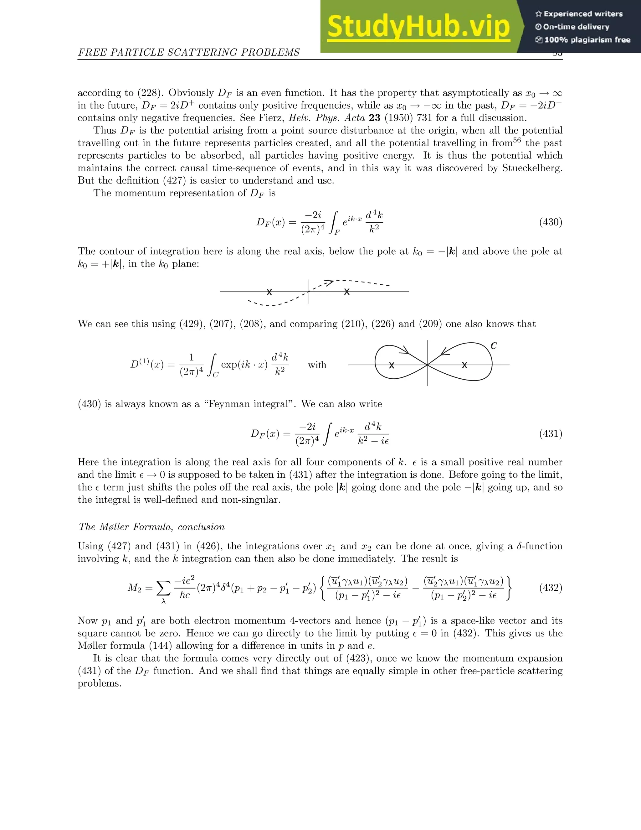
![FREE PARTICLE SCATTERING PROBLEMS 85
where SF is a new invariant function. Since
ǫ(x2 − x1)P
ψα(x1), ψβ(x2) = 1
2 [ ψα(x1), ψβ(x2) ] + 1
2 ǫ(x2 − x1)
ψα(x1), ψβ(x2) (443)
we have by (299) and (329)
SF (x) = S(1)
+ iǫ(x)S(x) (444)
in exact analogy to (429). We write also
SF (x) =
X
λ
γλ
∂
∂xλ
− µ
∆F (x) (445)
and we find from (444) the momentum representations
∆F (x) =
−2i
(2π)4
Z
eik·x d4
k
k2 + µ2 − iǫ
(446)
SF (x) =
2
(2π)4
Z
eik·x
/
k + iµ
k2 + µ2 − iǫ
d4
k (447)
We can also write (447) conveniently as
SF (x) =
2
(2π)4
Z
F
eik·x 1
/
k − iµ
d4
k (448)
Here the Dirac matrix in the denominator means that we have to multiply above and below by (/
k + iµ) in
order to evaluate the integral. Thus (448) is not a real simplification of (447), only it saves writing. The
Feynman integration in (448) is defined as a contour integral exactly as in (430).
Now substituting from (448) into (441), just like for (432)
M2 =
−e2
~2c2
(2π)4
δ 4
(p + k − p′
− k′
) u′
/
e
1
/
p − /
k
′
− iµ
/
e′
+ /
e′ 1
/
p + /
k − iµ
/
e
#
u (449)
Again the denominators (p − k)2
+ µ2
can never vanish so the ǫ can be put equal to zero in (447). In fact
if the electron is initially at rest
(p − k′
)2
+ µ2
= (p2
+ µ2
) + k′ 2
− 2p · k′
= 2p0k′
0 = 2µk′
0
and similarly
(p + k)2
+ µ2
= −2µk0 (450)
because k′ 2
= 0 and p2
= −µ2
; p = 0 because the electron is at rest.
M2 =
−e2
2~2c2µ
(2π)4
δ 4
(p + k − p′
− k′
) u′
1
k′
0
/
e(/
p − /
k
′
+ iµ)/
e′
−
1
k0
/
e′
(/
p + /
k + iµ)/
e
u (451)
Now we can simplify (451) further. Since the photon is not polarized in time, e4 = e′
4 = 0; since the electron
is at rest, p = 0. Hence e · p = 0, and thus /
e/
p = −/
p/
e + 2I e · p = −/
p/
e, i.e. /
p and /
e anticommute. This plus
the fact that u is a spin state of momentum ~p, i.e.
(/
p − iµ)u = 0 (452)
mean that the term /
p + iµ in (451) can be omitted. Thus we get
M2 =
e2
2~2c2µ
(2π)4
δ 4
(p + k − p′
− k′
) u′
/
e
/
k
′
k′
0
/
e′
+ /
e′ /
k
k0
/
e
#
u (453)](https://image.slidesharecdn.com/advancedquantummechanics-230806151100-7e1e8919/75/Advanced-Quantum-Mechanics-91-2048.jpg)
![FREE PARTICLE SCATTERING PROBLEMS 89
and so (464) is
e4
8~4c4µ4
2µ2
(k0 − k′
0)2
k0k′
0
+ 2µ(e · e′
) Spur
/
p/
eiβ/
e′
=
e4
4~4c4µ2
(k0 − k′
0)2
k0k′
0
+ 4(e · e′
)2
(465)
Hence by (461) the cross-section averaged over electron spins is
σ =
e4
k′2
0 dΩ
64π2~2c2µ2k2
0
(k0 − k′
0)2
k0k′
0
+ 4(e · e′
)2
The classical electron radius is
ro =
e2
4πmc2
=
e2
4π~cµ
Hence
σ = 1
4 r2
o dΩ
k′
0
k0
2
(k0 − k′
0)2
k0k′
0
+ 4 cos2
φ
(466)
where φ is the angle between the polarizations of the incident quantum k0 and the emitted quantum k′
0.
This is the famous Klein-Nishina formula.
To put σ explicitly as a function of the scattering angle θ, we must use the equations61
k · k′
= −µ(k0 − k′
0)
k · k′
= |k||k′
| cos θ − k0k′
0 = k0k′
0(cos θ − 1)
k0k′
0(1 − cos θ) = µ(k0 − k′
0)
k0
k′
0
= 1 + (1 − cos θ)
k0
µ
Put
ǫ =
k0
µ
=
Photon energy
mc2
Then
σ = 1
4 r2
o dΩ
(1 − cos θ)2
ǫ2
1 + ǫ(1 − cos θ)
+ 4 cos2
φ
[1 + ǫ(1 − cos θ)]
2 (467)
Thus for large ǫ the scattered photons are mainly unpolarized and concentrated in the forward direction.
For small ǫ (non-relativistic problem) we have simply62
σ = r2
o cos2
φ dΩ (468)
the classical result. Summing over the two polarizations of the photon k′
and averaging over all polarizations
of k, this gives the cross-section for all polarizations
σ = 1
2 r2
o(1 + cos2
θ) dΩ (469)
We get this by evaluating 1
2
P
e
P
e′ (e · e′
)2
. First we have to sum over the two polarization directions of
photon k′
. This summation for three directions would give
X
(e · e′
)2
= e2
= 1
Hence for the two directions perpendicular to k′
we can write
X
e′
(e · e′
)2
= 1 − (e · k̂
′
)2](https://image.slidesharecdn.com/advancedquantummechanics-230806151100-7e1e8919/75/Advanced-Quantum-Mechanics-95-2048.jpg)
![FREE PARTICLE SCATTERING PROBLEMS 91
For perpendicular polarizations, take coordinate axes 1 along e, 2 along e′
, and 3 along k. Then
(/
e/
k
′
/
e′
+ /
e′
/
k/
e) = µ{γ1(−γ3 + iβ)γ2 + γ2(γ3 + iβ)γ1} = 2µγ1γ2γ3 (476)
Hence for perpendicular polarizations64
u[/
e/
k
′
/
e′
+ /
e′
/
k/
e]u = 2µvT
Cγ4γ1γ2γ3u = −2µivT
γ4σ2u
= 2µvT
0 −1 0 0
1 0 0 0
0 0 0 1
0 0 −1 0
u
=
(
0 when spins u and v are parallel
2µ
√
2 when spins u and v are antiparallel
We get this latter result by observing that for antiparallel spins the initial wave function is
ψ =
1
√
2
1
0
0
1
−
1
√
2
0
1
1
0
(neglecting the “small components”) and therefore
vT
0 −1
1 0
u =
1
√
2
(0 1)
0 −1
1 0
1
0
−
1
√
2
(1 0)
0 −1
1 0
0
1
=
1
√
2
(1 0)
1
0
− (0 − 1)
0
1
=
2
√
2
=
√
2
This is one place where charge-conjugate spinors are useful and necessary!
Summarizing, we find for electron and positron with spins parallel, in triplet state, the 2-photon decay
is forbidden. This selection rule is in fact an exact one for positronium in the ground state 1s triplet. Only
3-photon decay can occur and this makes the lifetime ∼ 1100 times longer. For electron and positron in
singlet state, the 2-photon decay occurs with the photons always polarized perpendicularly to each other.
The probability for the decay, integrating (474) over a solid angle 2π since the photons are indistinguishable,
is
w =
~2
c3
16π
2|K|2
=
2e4
~2cµ28π
= 4πcr2
o (477)
Formula (477) is for electron and positron normalized to one particle per unit volume. If the density of the
electron probability relative to the position of the positron is ρ, then the mean annihilation life-time will
be65
(the “classical electron radius” ro = e2
/(4πmc2
) in Heaviside units)
τ =
1
4πcr2
oρ
(478)
For the positronium 1s singlet state
ρ =
1
8πa3
o
ao = Bohr radius = 1372
ro
τ = 2 × 1374
×
ao
c
= 2 × 1375
×
~
mc2
≈ 1.2 × 10⁻¹⁰
sec. (479)
For slowly-moving electrons and positrons with relative velocity v, the annihilation cross-section accord-
ing to (477) will be
4πr2
o
c
v
singlet state, (480)
proportional to
1
v
just like neutron cross-sections at low (thermal) energies.](https://image.slidesharecdn.com/advancedquantummechanics-230806151100-7e1e8919/75/Advanced-Quantum-Mechanics-97-2048.jpg)
![GENERAL THEORY OF FREE PARTICLE SCATTERING 96
The Reduction of an Operator to Normal Form
Given any operator O which is a product of field operators, for example
O = ψ(x1) /
A(x1)ψ(x1)ψ(x2) /
A(x2)ψ(x2) (496)
we want to pick out the matrix element of O for a transition between states A and B in which there is a
known distribution of bare particles. For example A may be a state with only one electron in state 1, and
B a state with one electron in state 2. Then we wish to pick out from (496) terms in which there appear
the operators b1 and b∗
2. In order to pick out all such terms systematically, we make a complete analysis of
O into a sum of terms On, each On being a sum of products of emission and absorption operators in which
all emission operators stand to the left of all absorption operators.69
. Any operator in which the emission
and absorption operators are arranged in this special way is called “Normal”70
[19]. The On will be called
the “Normal constituents” of O. Once O has been analyzed in this way, then we find the matrix element
simply by taking the coefficient of b∗
2b1 in the expansion
P
On. No other term in the expansion can give
any contribution to the matrix element. In O itself there might appear a term such as
b∗
2b3b∗
3b1 (497)
which would give a contribution to the matrix element, since the operator b∗
3 could create a particle in
an intermediate state 3 which the operator b3 would then annihilate. The expansion of O into normal
constituents eliminates all terms such as (497) and replaces them by sums of normal products with numerical
coefficients. Thus using the anticommutation rule for b3 and b∗
3, (497) becomes replaced by
Ab∗
2b1 − b∗
2b∗
3b3b1 (498)
where A is a numerical coefficient. The second term in (498) gives no contribution to the matrix element.
It is clear that by using the commutation rules of the operators in this way, every O can be written as
a sum of normal products, and that the analysis leads to a unique expansion of O. But we do not need
to go through the tedious algebra of using the commutation rules, instead we can write down the normal
constituents On directly by following simple rules.
First, we define the notation N(Q), where Q is any product of emission and absorption operators,
to be the product obtained by simply rearranging the factors of Q in a normal order, irrespective of the
commutation rules, with a factor (−1) if the rearrangement involves an odd permutation of the electron-
positron operators. Similarly if Q is any sum of products, N(Q) is defined by rearranging factors in each
term of the sum in the same way. Thus we have for example (see (211))
N(Aλ(x)Aµ(y)) = A+
λ (x)A+
µ (y) + A−
λ (x)A−
µ (y) + A−
λ (x)A+
µ (y) + A+
µ (y)A+
λ (x) (499)
where A+
µ (x) is the positive-frequency part of Aµ(x), i.e. the part containing absorption operators. Observe
that the order of factors in the first two products in (499) is immaterial, only the third and fourth products
have their order fixed by the condition of being normal. Similarly (see (306) and (309))
N ψα(x)ψβ(y)
= ψ +
α (x)ψ
+
β (y) + ψ −
α (x)ψ
−
β (y) + ψ −
α (x)ψ
+
β (y) − ψ
−
β (y)ψ +
α (x) (500)
With this notation, every product of two field operators can immediately be written as a sum of normal
constituents. Using the commutation rules (213) and the vacuum expectation values given by (219), (220),
Aλ(x)Aµ(y) = hAλ(x)Aµ(y)io + N(Aλ(x)Aµ(y)) (501)
Similarly, using (310), (311), (324),
ψα(x)ψβ(y) = ψα(x)ψβ(y) o
+ N ψα(x)ψβ(y)
(502)
And in fact for any two field operators P, Q we have
PQ = hPQio + N(PQ) (503)](https://image.slidesharecdn.com/advancedquantummechanics-230806151100-7e1e8919/75/Advanced-Quantum-Mechanics-102-2048.jpg)
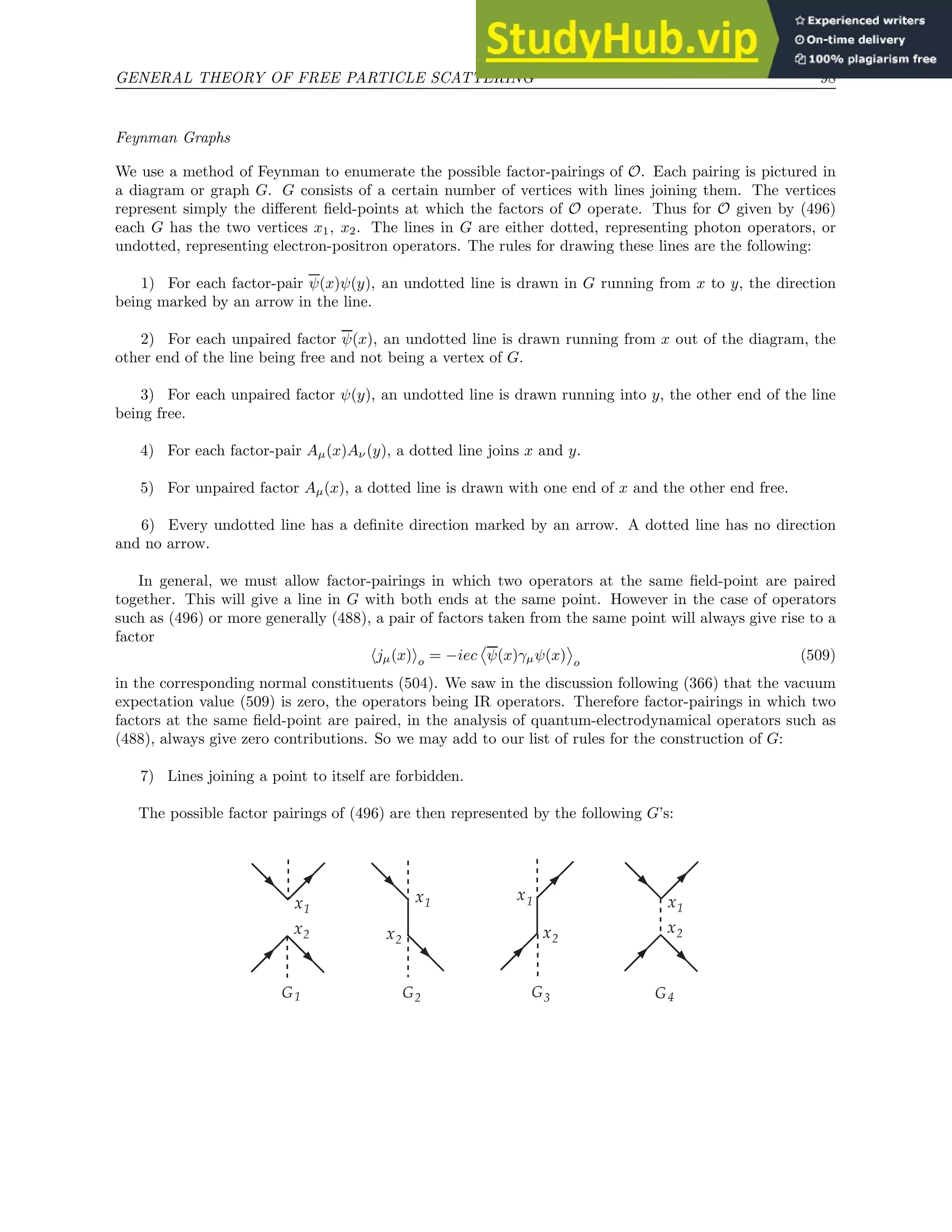
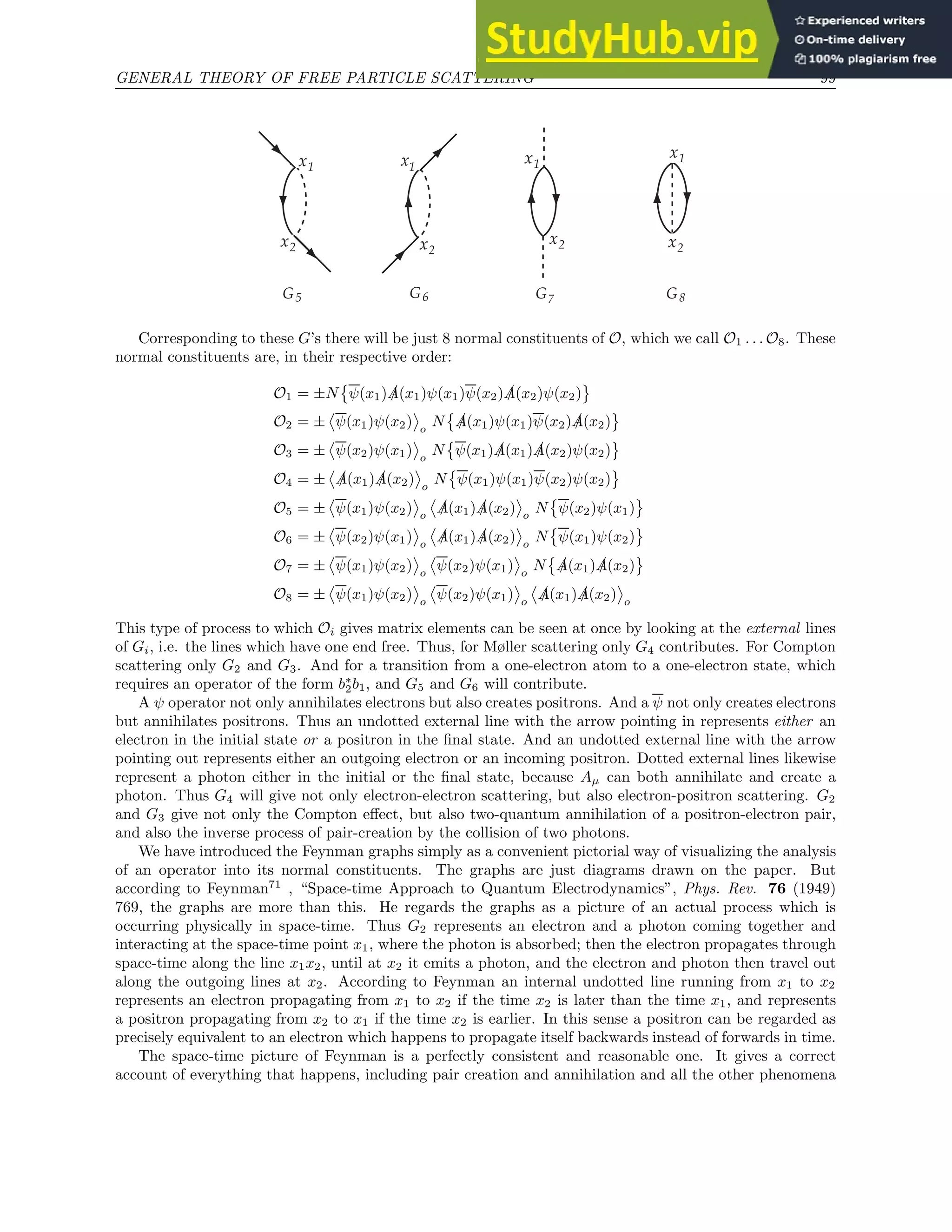
![GENERAL THEORY OF FREE PARTICLE SCATTERING 103
appearing in (519). Since (p, u) are the momentum and spin of a real electron, we may use the relations
p2
+ µ2
= 0, (/
p − iµ)u = 0 (521)
when we evaluate Σ(p) in (519). So using (376), (585) and following the same method that was used in
evaluating (377)74
Σ(p) =
Z
F
dk
X
λ
γλ(/
k + /
p + iµ)γλ
k2(k2 + 2p · k)
=
Z
F
dk
4iµ − 2/
k − 2/
p
k2(k2 + 2p · k)
= 2
Z 1
0
dz
Z
F
dK
iµ − /
k
[k2 + 2zp · k]2
= 2
Z 1
0
Z
F
dk
(iµ − /
k + z/
p)
[k2 − z2p2]2
= 2
Z 1
0
dz
Z
F
dk
iµ(1 + z)
[k2 + z2µ2]2
(522)
where we changed the origin of the k integration by the replacement k → k − zp and we eliminated the odd
terms. Using (386) and introducing the logarithmic divergence R again according to (387),
Σ(p) = 2
Z 1
0
dz iµ(1 + z){2iπ2
(R − log z)} = −π2
µ [6R + 5] = −6π2
µR′
(523)
Thus Σ(p) is a logarithmically divergent constant, depending only on the electron mass and independent
of the state of the electron. The difference 5/6 between R and R′
is of course not significant. Substituting
(523) into (519) gives the value of M2
M2 = −6π2
i
e2
µ
~c
R′
δ(p − p′
) (u′
u) (524)
Thus U2 does not give any transitions between different one-electron states. It has only the diagonal matrix
elements given by (524) .
Now (524) has precisely the correct relativistic form to be identified with a pure self-energy effect.
Suppose that in consequence of the radiation interaction the mass of a real electron is
m = mo + δm (525)
where mo is the mass of the bare electron without interaction and δm is the electromagnetic contribution
to the mass. The mass-change δm would be represented by a term
LS = −δm c2
ψψ (526)
in the Lagrangian density (410). This would produce an interaction energy
HS(t) = δmc2
Z
ψ(r, t)ψ(r, t) d3
r (527)
in the Schrödinger equation (415), and finally a contribution
US = −i
δmc
~
Z
ψψ(x) dx (528)
in the scattering matrix (421) or (488).
The matrix element of (528) between the states (pu) and (p′
u′
) is
MS = −i
δmc
~
(2π)4
δ(p − p′
) (u′
u) (529)](https://image.slidesharecdn.com/advancedquantummechanics-230806151100-7e1e8919/75/Advanced-Quantum-Mechanics-109-2048.jpg)
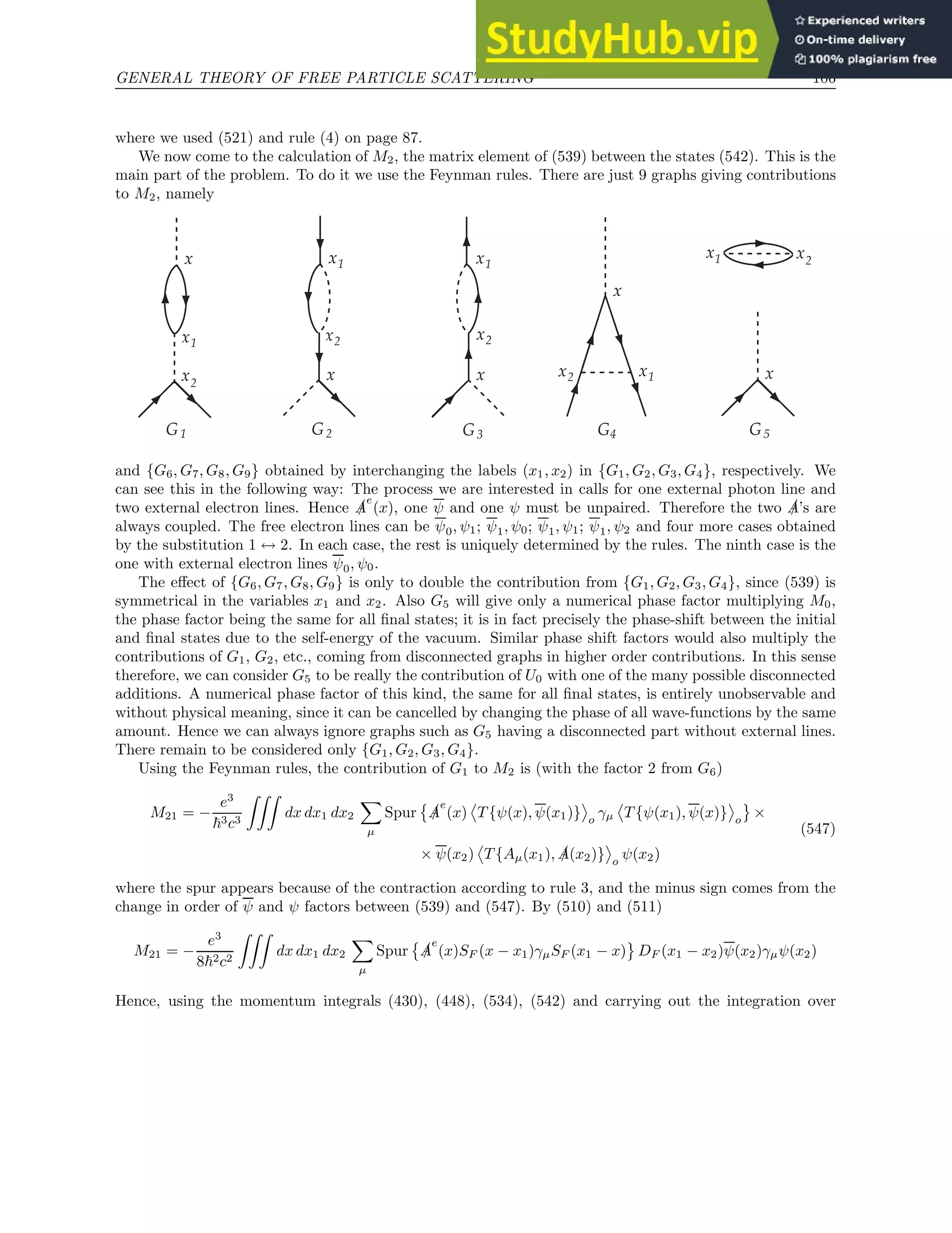
![GENERAL THEORY OF FREE PARTICLE SCATTERING 110
This is a convenient definition of I1 for future reference.
Now it is clear that the term R′
in M22 represents some kind of effect of the electron self-energy, which
ought not to be observable. We may expect that this term will be cancelled by the term M′
2 arising from
the self-energy correction HS in (532). This is all the more plausible, because the graph G2 on page 106
contains as a part the graph G5 on page 99 which represents the self-energy of a free electron. We now turn
to the calculation of M′
2.
M′
2 is the sum of two contributions arising from the two graphs shown below.
x1
G2
x
G3
x1
x
'
'
From G′
2 the contribution is (compare with (528))
M′
22 = −
ie δm
2~2
ZZ
dx dx1 ψ(x) /
A
e
SF (x − x1) ψ(x1) (574)
Like (555) this integral does not oscillate but diverges at t1 = ±∞. Therefore we must take explicitly
into account the cut-off factor multiplying the radiation interaction. At time t1 the radiation interaction
HR(t1) will carry the cut-off factor g(t1). But the self-energy δm at time t1 is an effect of second order
in HR, and therefore becomes multiplied by [g(t1)]
2
if g(t1) varies slowly enough. In the definition of the
scattering matrix element (487), the cut-off factors g(t) were introduced in order to represent the initial
and final states by simple bare-particle wave-functions in an unambiguous way. We now require that the
bare-particles’ wave-functions should always have the same mass m as a real electron. This is achieved if we
add the term (−HS) to the radiation interaction appearing in (495), each HS(ti) being multiplied by the
cut-off factor [g(ti)]2
so long as we are dealing only with second order terms in δm. If we were calculating
effects to fourth order in e, then the fourth order part of δm should be multiplied by [g(ti)]
4
, and so on.
The effect of the cut-off factors is therefore to replace (574) by
M′
22 = −
ie δm
2~2
ZZ
dx dx1 ψ(x) /
A
e
SF (x − x1) ψ(x1) [g(t1)]
2
(575)
Using (561) and performing the integrations as before, this becomes
M′
22 = −
ie δm
2~2
ZZ
G(ǫ0)G(ǫ′
0) dǫ0 dǫ′
0
(
u′
/
e(q − ǫ − ǫ′
)
1
/
p + /
ǫ + /
ǫ′
− iµ
!
u
)
(576)
In virtue of (530), this term does precisely cancel the term in R′
in (572), as was to be expected.
To simplify the term in I1 in (572), we may replace /
ǫ by 1
2 (/
ǫ + /
ǫ′
) since the integrand is otherwise
symmetrical between ǫ and ǫ′
. And using (521) we may replace this in turn by 1
2 (/
p + /
ǫ + /
ǫ′
− iµ). This
cancels the denominator of (572) precisely. After the denominator is cancelled, the expression is non-
singular and we may go to the limit T → ∞, using (563) to perform the integration over ǫ0 and ǫ′
0. Since
it is assumed that the external potential is of a limited duration not tending to infinity with T , the factor
/
e(q − ǫ − ǫ′
) is a continuous function of ǫ + ǫ′
and tends to /
e(q) as T → ∞.79
Hence in the limit T → ∞
we have
M22 + M′
22 =
ie3
(2π)4~2c2
1
2
I1 (u′
/
ǫu) =
iα
(2π)3
I1 Mo (577)](https://image.slidesharecdn.com/advancedquantummechanics-230806151100-7e1e8919/75/Advanced-Quantum-Mechanics-116-2048.jpg)
![GENERAL THEORY OF FREE PARTICLE SCATTERING 112
the table
X
λ
γλγλ = 4
X
λ
γλ/
aγλ = −2/
a
X
λ
γλ/
a/
bγλ = 4(a · b)
X
λ
γλ/
a/
b/
cγλ = −2/
c/
b/
a
(585)
valid for any vectors a, b, c. These formulae can be deduced from the following recursive formula:
Denote /
q(n)
= /
q1/
q2
. . . /
qn
where qi are arbitrary vectors, and χn =
P
λ γλ/
q(n)
γλ, χo = 4. Then we have
χn+1 =
X
λ
γλ/
q(n)/
qn+1
γλ =
X
λ
X
µ
γλ/
q(n)
γµγλ(qn+1)µ =
X
λ
X
µ
γλ/
q(n)
[2δλµ − γλγµ] (qn+1)µ
= 2/
qn+1/
q(n)
− χn/
qn+1
which then gives (585) for n = 1, 2, 3. Thus
Λ(p, p′
) = −2
Z
F
dk
(/
k + /
p)/
e(/
k + /
p′
) − 2iµ(2e · k + e · p + e · p′
) − µ2
/
e
k2 [k2 + 2k · p′] [k2 + 2k · p]
(586)
In (583) we may use the relations
p2
+ µ2
= p′2
+ µ2
= 0 (/
p − iµ)u = 0 u′
(/
p′
− iµ) = 0 (587)
We also assume that the external potential satisfies the Lorentz condition
X
λ
∂Ae
µ
∂xµ
= 0 so that e · q = 0 (588)
To evaluate (586) we use the 3-variable generalization of (376)
1
abc
= 2
Z 1
0
dx
Z 1
0
x dy
1
[a(1 − x) + bxy + cx(1 − y)]
3 (589)
which one can verify at once by direct integration. We write
py = py + p′
(1 − y)
p2
y = [−(p′
− p)y + p′
]2
= q2
y2
− (2p′2
− 2p · p′
)y − µ2
= q2
y2
− (p′2
− 2p · p′
+ p2
) − µ2
= −µ2
− (y − y2
)q2
(590)
Then changing the origin of the k-integration by the substitution k → k − xpy (586) and (589) give
Λ(p, p′
) = −4
ZZ
x dx dy
Z
F
dk
(/
k − x/
py
+ /
p)/
e(/
k − x/
py
+ /
p′
) − 2iµe · (2k − 2xpy + p + p′
) − µ2
/
e
k2 − x2p2
y
3 (591)
In (591) we may drop terms which are odd in k. Also using (587) and (588) we may put
e · p = e · p′
= e · py = iµ/
e + 1
2 /
e/
q (592)](https://image.slidesharecdn.com/advancedquantummechanics-230806151100-7e1e8919/75/Advanced-Quantum-Mechanics-118-2048.jpg)
![GENERAL THEORY OF FREE PARTICLE SCATTERING 113
(/
p − x/
py
)/
e(/
p′
− x/
py
) =
(1 − x)iµ − (1 − xy)/
q /
e
(1 − x)iµ + (1 − x + xy)/
q
= −(1 − x)2
µ2
/
e + (1 − x)iµ/
e/
q(2 − x) + (1 − xy)(1 − x + xy)q2
/
e
(593)
Collecting terms from (592), (593), we have
Λ(p, p′
) = −4
ZZ
x dx dy
Z
F
dk
/
k/
e/
k + (1 − xy)(1 − x + xy)q2
/
e − (x − x2
)iµ/
e/
q + (2 − 2x − x2
)µ2
/
e
[k2 + x2 (µ2 + (y − y2) q2)]3 (594)
Now we saw earlier that the integral (567), evaluated using the conditions p2
+ µ2
= 0, /
p − iµ = 0, has
the value (573). Comparing (567) with (584), this implies that
Λ(p, p) = Λ(p′
, p′
) = I1 /
e (595)
when the conditions (587) with p′
= p are assumed to hold. Thus (I1/
e) is just the value of (594) for p′
= p.
Adding together (583) and (578), this gives
M2T = M24 + M22 + M′
22 + M23 + M′
23 = −
ie3
(2π)4~2c2
(u′
Λc(p, p′
)u) (596)
Λc(p, p′
) = Λ(p, p′
) − 1
2 {Λ(p, p) + Λ(p′
, p′
)}
= −4
ZZ
x dx dy
(Z
F
dk
/
k/
e/
k + (2 − 2x − x2
)µ2
/
e
1
[k2 + x2 (µ2 + (y − y2) q2)]3 −
1
[k2 + x2µ2]3
!
+
(1 − xy)(1 − x + xy)q2
/
e − (x − x2
)iµ/
e/
q
Z
F
dk
1
[k2 + x2 (µ2 + (y − y2) q2)]
3
)
(597)
The k-integrals in (597) are now convergent. Thus the effect of the “wave-function renormalization” term
(578) is just to cancel out the part of M24 which is independent of q and divergent at high frequencies.
To evaluate (597) we use (385) and (386). First, in the term /
k/
e/
k we may replace kµkν by 1
4 δµνk2
because
of the symmetry of the integral in k-space. So we may write, using (585)
/
k/
e/
k =
X
α
1
4 k2
γα/
eγα = −1
2 k2
/
e (598)
Then by (385) and (386)
Z
F
dk k2
(
1
[k2 + Λ]
3 −
1
[k2 + Λ′]
3
)
=
=
Z
F
dk k2
(
1
[k2 + Λ]2 −
1
[k2 + Λ′]2 −
Λ
[k2 + Λ]3 +
Λ′
[k2 + Λ′]3
)
= π2
i log
Λ′
Λ
(599)
and (597) becomes
Λc(p, p′
) = 2π2
i
ZZ
x dx dy
−/
e log
1 + (y − y2
)
q2
µ2
+
{x − 1 + 2(y − y2
)(1 − x − x2
)}q2
/
e + (x − x2
)iµ/
e/
q
x2(µ2 + (y − y2) q2
)
Integrating the logarithmic term by parts with respect to y,
Λc(p, p′
) = −2π2
i
Z 1
0
Z 1
0
dx dy
1
x [µ2 + (y − y2) q2]
(1 − x)(1 − 2y + 2y2
) + x2
y
q2
/
e − (x − x2
)iµ/
e/
q
(600)](https://image.slidesharecdn.com/advancedquantummechanics-230806151100-7e1e8919/75/Advanced-Quantum-Mechanics-119-2048.jpg)
![GENERAL THEORY OF FREE PARTICLE SCATTERING 114
When q2
−4µ2
, the external potential is able to create real pairs, and the denominator in (600) has
poles in the range of the y-integration. In this case the Feynman rule of adding a term (−iǫ) to µ2
, where ǫ
is an infinitesimal positive real number, will give an unambiguous determination of the integral. Just as in
the case of the vacuum polarization formula (389), the integral will split into a real part and an imaginary
part describing the effects of the real pairs created. We shall not discuss these effects of real pairs since
they are not practically important. So we assume q2
−4µ2
.
In (600) there are no longer any divergences arising from large k. But (584) has a logarithmic divergence
at small k which appears in (600) as a divergence in the x-integration arising from the factor (1/x). This
last remaining divergence must now be examined in detail. It is the famous “Infra-Red Catastrophe”.
To discover the physical meaning of the x-divergence, we consider what would be the effect on our
calculations if the Maxwell field were somehow modified so that all field oscillations with wave-numbers
satisfying
|k| ≥ r (601)
were present as usual, while all oscillations not satisfying (601) were simply absent or incapable of being
excited. We suppose r to be a constant small compared with m, p, p′
and q. Thus photons will exist only
if their energies exceed
∆E = ~cr (602)
In the modified Maxwell theory the DF function will still be given by the integral (431), the k1, k2, k3
integrations being limited by (601), and the k0 integration being taken as usual along the whole real axis
from −∞ to +∞. Let Λr
(p, p′
) and Λr
c(p, p′
) be the integrals which replace Λ(p, p′
) and Λc(p, p′
) when the
Maxwell field is modified. We calculate the differences (Λ − Λr
) and (Λc − Λr
c), considering these integrals
only in the limit of small r, neglecting all terms which tend to zero with r. This means that we may neglect
terms containing either k or x as a factor in the numerator of integrals such as (591) or (594).
In (583) there is just one factor DF . Thus Λr
(p, p′
) is obtained from (584) simply by restricting the
k1, k2, k3 integration by (601). We can now follow the reduction of (584) to the form (594), except that
we do not shift the origin of the k-integration through (xpy) since this would disturb the condition (601).
Dropping terms in the numerator having k or x as a factor, this gives the result
Λ(p, p′
) − Λr
(p, p′
) = −4
ZZ
x dx dy (q2
+ 2µ2
)/
e
Z
F
dk
[k2 + 2xk · py]3 (603)
Hence by (597)
Λc(p, p′
) − Λr
c(p, p′
) =
= −4
ZZ
x dx dy /
e
Z
F
dk
(
q2
+ 2µ2
[k2 + 2xk · py]
3 −
µ2
[k2 + 2xk · p]
3 −
µ2
[k2 + 2xk · p′]
3
)
(604)
The integral (604), with the integration extended over the whole k-space, would give, using (385), (587),
and the substitutions k → k − xpy, k → k − xp, k → xp′
, respectively in the three integrals,
−2πi
ZZ
dx dy
(1 − 2y + 2y2
) q2
x(µ2 + (y − y2) q2)
/
e (605)
which is just the divergent part of (600). But the integration in (604) actually extends over k not satisfying
(601). Therefore subtracting (604) from (600) and using (605), we find for Λr
c(p, p′
) the final result
Λr
c(p, p′
) = −2π2
i
Z 1
0
dy
1
µ2 + (y − y2) q2
(−1 + 5
2 y − 2y2
) q2
/
e − 1
2 iµ/
e/
q
− 4
ZZ
x dx dy /
e
Z
F
dk
(
q2
+ 2µ2
[k2 + 2xk · py]
3 −
µ2
[k2 + 2xk · p]
3 −
µ2
[k2 + 2xk · p′]
3
) (606)](https://image.slidesharecdn.com/advancedquantummechanics-230806151100-7e1e8919/75/Advanced-Quantum-Mechanics-120-2048.jpg)
![GENERAL THEORY OF FREE PARTICLE SCATTERING 115
This integral is completely convergent for every finite r, the k-integration being restricted to k satisfying
(601). The formula (606) is exact except for terms which tend to zero with r.
To evaluate the k integral in (606) for general p and p′
is possible but tedious. So we shall do it only in
the case of non-relativistic velocities, when
|p| ≪ µ, |p′
| ≪ µ, |q| ≪ µ (607)
where |p| means
p
p2
1 + p2
x + p2
3, the magnitude of the space-like part of the 4-vector p. In addition to (607)
we still assume r small compared to q, p, p′
.
We consider the integral
K =
Z 1
0
Z 1
0
x dx dy
Z
F
dk
1
[k2 + 2xk · py]
3 (608)
integrated over k satisfying (601), and evaluate it including terms of order |p|2
, q2
, |p′
|2
, but neglecting
higher terms. Integrating over k0 only, we have for any positive b
Z
F
dk0
1
[k2 + 2ak0 + b]
= i
Z ∞
−∞
dk0
[|k|2 + k2
0 + 2iak0 + b]
= iπ
1
p
|k|2 + a2 + b
(609)
Differentiating (609) twice with respect to b,
Z
F
dk0
[k2 + 2ak0 + b]
3 =
3iπ
8
|k|2
+ a2
+ b
−5/2
(610)
Hence80
K =
ZZ
x dx dy
3iπ
8
Z
|k|r
d3
k
|k + xpy|2
+ x2
µ2
+ (y − y2
) q2
−5/2
=
ZZ
x dx dy
3iπ
8
Z
|k|r
d3
k
n
|k|2
+ x2
µ2
−5/2
− 5
2 2xk · py + x2
|py|2
+ x2
(y − y2
) q2
×
|k|2
+ x2
µ2
−7/2
+ 35
8 4x2
(k · py)2
|k|2
+ x2
µ2
−9/2
o
=
ZZ
x dx dy
3iπ2
2
Z ∞
r
k2
dk
n
k2
+ x2
µ2
−5/2
− 5
2 x2
|py|2
+ (y − y2
) q2
k2
+ x2
µ2
−7/2
+35
6 x2
k2
|py|2
k2
+ x2
µ2
−9/2
o
(611)
We can now carry out the integrations over x and y, using
Z 1
0
|py|2
dy = p · p′
+ 1
3 q2
(612)
This gives
K =
3iπ2
2
Z ∞
r
k2
dk
1
3µ2
1
k3
−
1
(k2 + µ2)3/2
−
p · p′
+ 1
2 q2
3µ4
1
k3
−
1
(k2 + µ2)3/2
−
1
2µ2(k2 + µ2)5/2
+ 1
6 k2
p · p′
+ 1
3 q2
2
µ4
1
k5
−
1
(k2 + µ2)5/2
−
5
µ2
1
(k2 + µ2)7/2
(613)
The k-integration is now elementary, and after dropping terms which tend to zero with r we have
K =
3iπ2
2µ2
1
3
log
µ
2r
+ 1
−
p · p′
+ 1
2 q2
µ2
1
3 log
µ
2r
+ 1
6
+ 1
6
p · p′
+ 1
3 q2
µ2
2 log
µ
2r
+ 5
3
(614)](https://image.slidesharecdn.com/advancedquantummechanics-230806151100-7e1e8919/75/Advanced-Quantum-Mechanics-121-2048.jpg)
![GENERAL THEORY OF FREE PARTICLE SCATTERING 116
Putting p = p′
, q = 0 in (614), we find
K0 =
Z 1
0
Z 1
0
x dx dy
Z
F
dk
1
[k2 + 2xk · p]3
=
3iπ2
2µ2
1
3
log
µ
2r
+ 1
+ 1
9
|p|2
µ2
(615)
Substituting (614) and (615) into (606) and dropping terms of higher order than |p|2
, |p′
|2
and q2
,
Λr
c(p, p′
) = −2π2
i
− 5
12
q2
µ2
/
e − 1
2
i
µ
/
e/
q
− 4/
e
3iπ2
2µ2
n
1
3 q2
log
µ
2r
+ 1
− 1
18 q2
2 log
µ
2r
+ 5
3
o
= −4
3 π2
i
q2
µ2
/
e
n
log
µ
2r
+ 11
24
o
−
π2
µ
/
e/
q
(616)
Using (596) and adding the contribution (554) from G1, we find for the second-order terms in (541) the
value
M2 + M′
2 = −
α
3π
n
log
µ
2r
+ 11
24 − 1
5
o q2
µ2
M0 +
α
4π
ie
mc2
u′
/
e/
qu
(617)
The Treatment of Low-Frequency Photons. The Infra-Red Catastrophe.
The second-order correction (617) to the scattering matrix element M0 has been made convergent by only
taking into account the effects of photons with energy greater than ∆E according to (603). When ∆E → 0
the correction diverges logarithmically, and this divergence must now be interpreted.
In the approximation where |p|2
and |p′
|2
are small compared with µ2
, (546) gives
M1 =
e
~cµ|k′
|
(q · e′
)M0 (618)
The total probability that an electron is scattered between the initial and final states (542), with the
emission of a photon with potentials (440), summed over all photons with frequencies lying in the range81
r1 |k′
| r2 (619)
is therefore
WR(r1, r2) =
Z
d3
k′
X
e′
1
(2π)3
~c
2|k′
|
|M1|2
=
e2
16π3~cµ2
|M0|2
Z
d3
k′ 1
|k′
|3
X
e′
|q · e′
|2
=
α
πµ2
|M0|2
Z r2
r1
dk′
k′
2
3 q2
=
2α
3π
log
r2
r1
q2
µ2
|M0|2
(620)
In (620) it is assumed that both r2 and r1 are frequencies small compared with |q|.
On the other hand, the probability that an electron is scattered between the states (542) without
emitting a photon is given by
WN = |M0 + M2 + M′
2|2
= |M0|2
+ M∗
0 (M2 + M′
2) + (M2 + M′
2)
∗
M0
(621)
neglecting terms of fourth order in the radiation interaction. If we consider in (621) the contribution only
from virtual photons with frequencies in the range (619), then by (617) we have
M2 + M′
2 = −
α
3π
log
r2
r1
q2
µ2
|M0|2
WN (r1, r2) = |M0|2
−
2α
3π
log
r2
r1
q2
µ2
|M0|2
(622)](https://image.slidesharecdn.com/advancedquantummechanics-230806151100-7e1e8919/75/Advanced-Quantum-Mechanics-122-2048.jpg)
![SCATTERING BY A STATIC POTENTIAL 121
Formula (646) gives a result of the form
σT =
1 −
8α
3π
β2
sin2 θ
2
log
mc2
2T
+ f(θ)
σ0 (647)
where for low velocities f(θ) is independent of T and of order 1 compared to the logarithm. For any special
potential f(θ) can be calculated.
From (647) we see that the observable radiative correction is not of order α but of order
α
v
c
2
log
c
v
(648)
which is much smaller if v is not relativistic. Thus the correction cannot be observed at all in a non-
relativistic scattering experiment. In the relativistic region the effect is actually of order α as indicated by
(647), but the correct formula is then enormously more complicated.
The exact formulae in both non-relativistic and relativistic cases have been published by J. Schwinger,
Phys. Rev. 76 (1949) 790.
An experimental test in the relativistic range is just on the limits of the possible. See Lyman, Hanson
and Scott, Phys. Rev. 84 (1951) 626. Scattering of 15 MeV electrons by nuclei were measured with very
good energy-resolution, ∆E/E being 1 - 3 %. In this case it was only the non-radiative cross-section σN
that was observed, and so the radiative correction given by the relativistic form of (637) becomes quite
large. In fact the radiative correction in σN in the relativistic range becomes of the order
α
log
∆E
E
log
E
mc2
(649)
according to Schwinger, Phys. Rev. 76, 813, Eq. (2.105) (with misprint K for k, in my notation µ.) In
the conditions of the experiment of Lyman-Hanson-Scott (649) becomes of the order 5% and was clearly
observed, the experimental errors being ∼ 2%. However, (649) arises mainly from the low-energy virtual
photons, with energies going down to ∆E. What is observed is just the decrease in the non-radiative
cross-section due to the competition of radiative scattering with energy-loss in the range [∆E, E]. Thus
the measurement of (649) by LHS is actually only a very inaccurate measurement of the cross-section for
bremsstrahlung, which could be observed much more accurately by observing the photons which are really
emitted.
The theoretically interesting part of the radiative corrections is the part which is not just the effect
of real bremsstrahlung. This part is given by the terms in σN which are of order 1 compared with the
log(∆E/E) appearing in (649). For example, we would have to observe with sufficient accuracy to see the
terms (5
6 − 1
5 ) in (637) if we wished to verify the theoretical radiative corrections at low velocities. In the
relativistic range the “genuine” radiative corrections are of order
α log
E
mc2
(650)
instead of (649), i.e. about 2% in the LHS experiment. To detect such effects is already possible, but to
observe them accurately in a scattering experiment seems not very hopeful.
This is all we can say at present about radiative corrections to scattering by an electrostatic potential.
A. The Magnetic Moment of the Electron
The scattering by an electrostatic potential, the two terms in (617) were lumped together. Both gave
contributions of the same order of magnitude, α(q2
/µ2
) in the cross section. What then is the meaning of
the special form of the second term in (617)? This term has no infra-red divergence and therefore should
be particularly simple to interpret experimentally.](https://image.slidesharecdn.com/advancedquantummechanics-230806151100-7e1e8919/75/Advanced-Quantum-Mechanics-127-2048.jpg)


![SCATTERING BY A STATIC POTENTIAL 124
with HI
given by (532) including the mass-renormalization term HS. The first stage in the solution of
(661) is to write
Ψ(t) = Ω1Φ(t) (662)
where Ω1(t) is defined as in (492), only with eψ /
Aψ replaced by [eψ /
Aψ + i δm c2
ψψ], and the function gA(t)
is as before supposed to tend to the limiting form gA(t) → 1 at the end of the calculation. The operator
Ω1(t) satisfies
i~
∂ Ω1(t)
∂t
= HI
(t) Ω1(t) (663)
for any value of t not in the remote past, so that we may take gA(t) = 1. Hence the equation of motion for
Φ(t) derived from (661) is just
i~
∂Φ
∂t
= HT (t)Φ (664)
HT (t) = (Ω1(t))
−1
He
(t) Ω1(t) (665)
The covariant part of the calculation, which is done in the FIR, is just the evaluation of this transformed
Hamiltonian HT (t).
Covariant Part of the Calculation
Let us write
HF (t) = Ω2(t) He
(t) Ω1(t) (666)
with Ω2 given by (490). Then
HT (t) = (Ω2(t)Ω1(t))
−1
HF (t) = S−1
HF (t) (667)
where S, given by (495), is the scattering matrix defined in the absence of the external potential Ae
µ. We
shall now restrict our attention to systems in which only one electron is actually present. We saw by Eq.
(533) that S applied to a one-electron state is equivalent to the unit operator, i. e.g. S produces no real
scattering or shift of phase in one-particle states. Therefore in discussing the hydrogen atom we may simply
omit the S−1
in (667) and write
HT (t) = HF (t) (668)
Now HF (t) is just the term involving He
(t) in the series expansion (421). In fact we have, by direct
multiplication of the series for Ω1 and Ω2,
HF (t) =
∞
X
n=0
−i
~
n
1
n!
Z
. . .
Z
dt1 dt2 . . . dtn P
He
(t), HI
(t1), . . . , HI
(tn) (669)
the damping functions g(ti) being always understood when they are not written explicitly. Now (667) is
directly related to the operator U given by (535), namely
U = −
i
~
Z ∞
−∞
HF (t) dt (670)
We write
HT (t) = He
(t) + HT 1(t) + HT 2(t) (671)
expanding HT in powers of the radiation interaction just as U was expanded in (536)–(540). But the matrix
elements of U2 + U1
2
referring to one-electron transition have already been calculated and are given by
(617) assuming non-relativistic velocities for the electron. This enables us to write down immediately a](https://image.slidesharecdn.com/advancedquantummechanics-230806151100-7e1e8919/75/Advanced-Quantum-Mechanics-130-2048.jpg)
![SCATTERING BY A STATIC POTENTIAL 127
(662) is only a transformation from one set of variables to another within the FIR, and does not take us
out of the FIR. This point was never explained properly by Schwinger in his papers, although he no doubt
understood it himself.
Let then Q(x) be a field-operator of the Ψ representation. Being a FIR operator, Q(x) satisfies
i~
dQ
dt
= [Q, H0] (685)
where H0 is the Hamiltonian of the Dirac and Maxwell fields without interaction. In the Φ representation
the corresponding field-operator is
Q′
(x) = (Ω1(t))
−1
Q(x) Ω1(t) (686)
Now Ω1(t) is given by (492) where we now take the limit gA = 1. The operators appearing in (492) are all
FIR operators satisfying equations of motion of the form (685). When the integrations in (492) are carried
out, the integrated terms will still have the same time variation given by (685), except for those terms
which correspond to transitions in which energy is conserved. The energy-conserving matrix elements will
have an explicit linear dependence on t after integration, which is not in accordance with (685). Therefore
we conclude that the equation of motion
i~
dΩ1
dt
= [Ω1, H0] (687)
is valid for all matrix elements of Ω1 which are not diagonal in the FIR. The same equation of motion
is satisfied by (Ω1(t))
−1
with the same condition. Now we have seen that Ω1(t) has no matrix elements
diagonal in H0 which give transitions either from or into one-particle states. Hence (687) holds for all
matrix elements in which either initial or final state is a one-particle state.
Combining (687) and the corresponding equation for (Ω1)
−1
with (685) and (686), we have
i~
dQ′
dt
= [Q′
, H0] (688)
This equation (688) is valid for all matrix elements between one-particle states. Thus we can conclude that
so long as we confine attention to a one-electron system, (688) is satisfied by all field operators of the Φ
representation, and so the Φ representation is still within the FIR.
When we consider systems containing more than one particle, then Ω1(t) will have an explicit dependence
on time in addition to (687). Then the Φ representation would no longer belong to the FIR. And this is
physically reasonable, because in many-electron systems it is not in general possible to transform away the
radiation interaction completely, the radiation interaction by itself giving rise to real effects such as Møller
scattering which we should not wish to transform away.
Concluding Non-Covariant Part of the Calculation
Having established that the Φ-representation in which (664) holds is the FIR, we now proceed at once to
transform to the BIR in which we shall finish the calculation of the Lamb shift. To transform to the BIR,
we write
Φ(t) = eiH0t/~
e−i{H0+He
}t/~
Φ′
(t) (689)
The new wave-function Φ′
(t) thus satisfies
i~
∂Φ′
∂t
= {HT 1(t) + HT 2(t)} Φ′
(690)
where HT 1 and HT 2 are given by (684) and (676), only now the ψ∗
and ψ operators have the time-variation
of the Dirac field in the external potential V .](https://image.slidesharecdn.com/advancedquantummechanics-230806151100-7e1e8919/75/Advanced-Quantum-Mechanics-133-2048.jpg)
![SCATTERING BY A STATIC POTENTIAL 128
To solve (690) we may now use precisely the method that we used for solving (245) in the non-relativistic
treatment. There are only two differences, (i) we have now the extra term HT 2, and (ii) the form of HT 1
is different form (247).
Since we are working only to second order in the radiation interaction and HT 2 is already of that order,
HT 2 is to be treated only as a first-order perturbation. Then HT 2 will have no effect on the line-width Γ,
and will contribute to the line-shift ∆E just the expectation-value of (676) in the state ψ0 of the atom,
namely
∆E2 =
α
3πµ2
n
log
µ
2r
+ 11
24 − 1
5
o Z
(∇2
V )|ψ0|2
d3
r −
iα
4πµ
Z
ψ∗
0γ4(α · ∇V )ψ0 d3
r (691)
The effect of the change from (247) to (684) is that the matrix element jk
µ(n m) given by (256) now
becomes everywhere replaced by
Jk
µ(n m) =
ie
~µ|k|
Z
ψ∗
n
∂V
∂xµ
e−ik·r
ψm d3
r (692)
We see this by comparing (247) and (684), noting that
j(r, t) ↔
ec
~µ
ψ∗
ψ∇V
Z
dt
or Z
jS
(r) e−ik·r
d3
r ↔
iec
~µ|k|c
Z
ψ∗
ψ ∇V e−ik·r
d3
r
In the previous calculation we used a non-relativistic dipole approximation for jµ which gave according to
(272)
jk
µ(n m) = +
ie~
m
Z
ψ∗
n
∂ψ
∂xµ
d3
r (693)
We shall again use a dipole approximation and drop the exponential factor in (692). Then taking for the
atom the non-relativistic Hamiltonian
H =
p2
2m
+ V (694)
the difference between (692) and (693) becomes
Jk
µ(n m) − jk
µ(n m) =
ie
~µ|k|
Z
ψ∗
n
∂ψ
∂xµ
d3
r
(Em − En − hc|k|) (695)
where we used [ p2
, pµ ] = 0 and
R
pµψ∗
n p2
ψm d3
r = −
R
ψ∗
n pµp2
ψm d3
r. This difference vanishes for
transitions in which energy is conserved. Hence the value of Γ given by (262) is unaffected by the change
from j to J. The value Γ calculated previously is still valid in the relativistic theory, except for very small
effects from magnetic radiation which we have neglected.
Using (695) we have the simple relation between jµ and Jµ,
Jk
µ(n m) = jk
µ(n m)
Em − En
hc|k|
(696)
Using formula (261) with J substituted for j, the contribution from HT 1 to the line-shift becomes instead
of (273)
∆E1 = −
e2
6π2m2~c3
Z ∞
r
dk
k
X
n
(En − E0)2
|pn0|2
En − E0 + hc|k|
(697)
The integral is now convergent at high frequencies and only divergent at low frequencies where the cut-off
r is now required to make it finite. The shift (697) would be zero for a free particle, and so there is no
question of subtracting away a mass-renormalization term as we did from (273); in the relativistic treatment
the mass-subtraction was already done long before this stage of the calculation was reached.](https://image.slidesharecdn.com/advancedquantummechanics-230806151100-7e1e8919/75/Advanced-Quantum-Mechanics-134-2048.jpg)
![SCATTERING BY A STATIC POTENTIAL 129
Integrating (697) directly over k, and taking r to be small compared with (En − E0), we find
∆E1 = −
e2
6π2m2~c3
X
n
(En − E0)2
|pn0|2
log
|En − E0|
hcr
(698)
This is precisely the non-relativistic line-shift (278) with r substituted for K. Defining (E − E0)av by (279)
and using (281), we have
∆E1 =
α
3πµ2
log
hcr
(E − E0)av
Z
(∇2
V ) |ψ0|2
d3
r (699)
This combines with (691) to give for the total level shift
∆E =
α
3πµ2
log
mc2
2(E − E0)av
+ 11
24 − 1
5
Z
(∇2
V ) |ψ0|2
d3
r −
iα
4πµ
Z
ψ∗
0 γ4(α · ∇V )ψ0 d3
r (700)
a result which is completely divergence-free and independent of r.
The second term of (700) represents the effect of the anomalous magnetic moment of the electron on
the energy levels. It therefore gives a spin-dependent shift which modifies slightly the fine-structure which
arises from the Dirac magnetic moment. To evaluate this term we use the Dirac equations (see (38)).
mc2
γ4ψ0 = (E0 − V )ψ0 + i~c(α · ∇)ψ0 (701)
mc2
ψ∗
0 γ4 = ψ∗
0 (E0 − V ) − i~c(∇ψ∗
0 · α) (702)
Using both (701) and (702) in turn in the second term of (700) and adding the results using αi
γ4 +γ4αi
= 0
the terms in (E0 − V ) cancel and we find93
2mc2
Z
ψ∗
0 γ4(α · ∇V )ψ0 d3
r
= −i~c
Z
{(∇ψ∗
0 · α)(α · ∇V )ψ0 + ψ∗
0(α · ∇V )(α · ∇ψ0)} d3
r
= −i~c
Z
{(∇ψ∗
0 · σ)(σ · ∇V )ψ0 + ψ∗
0 (σ · ∇V )(σ · ∇ψ0)} d3
r
= −i~c
Z
{ψ0 [∇ψ∗
0 · ∇V + iσ · (∇ψ∗
0 × ∇V )] + ψ∗
0 [∇ψ0 · ∇V + iσ · (∇ψ0 × ∇V )]} d3
r
= i~c
Z
+(∇2
V )ψ∗
0ψ0 − 2iψ∗
[σ · (∇V × ∇)]ψ0 d3
r
(703)
Here we used αi
= ǫσi (see p. 20), ǫ2
= I, and the formula
(σ · B)(σ · C) = (B · C) + i(σ · B × C)
See Dirac, The Principles of Quantum Mechanics, third edition, p. 263.
Now suppose V is a central potential, a function of r only. Then
∇V × ∇ =
1
r
dV
dr
(r × ∇) =
1
r
dV
dr
i
~
L
(704)
with L, the orbital angular momentum, is given by (39). In this case (700) becomes
∆E =
α
3πµ2
log
mc2
2(E − E0)avg
+ 5
6 − 1
5
Z
(∇2
V ) |ψ0|2
d3
r
+
α
4πµ2~
Z
ψ∗
0
1
r
dV
dr
(σ · L) ψ0 d3
r
(705)](https://image.slidesharecdn.com/advancedquantummechanics-230806151100-7e1e8919/75/Advanced-Quantum-Mechanics-135-2048.jpg)
![SCATTERING BY A STATIC POTENTIAL 130
In the non-relativistic theory of the hydrogen atom, the quantum number j given by (72) is related to the
operator (σ · L) by
1
~
(σ · L) =
(
ℓ, j = ℓ + 1
2
−ℓ − 1, j = ℓ − 1
2
(706)
Therefore for the hydrogen atom
∆E =
αe2
3πµ2
log
mc2
2(E − E0)avg
+ 5
6 − 1
5
|ψ0(0)|2
+
αe2
16π2µ2
q
Z
1
r3
|ψ0|2
d3
r (707)
where q is the coefficient (706).
For s-states we have q = 0 and so the shift reduces to (see (284))
∆E =
8α3
3π
1
n3
Ry
log
mc2
2(E − E0)avg
+ 5
6 − 1
5
(708)
for the state with principal quantum number n. For all other states the term in |ψ0(0)|2
is zero, and the
shift depends only on the integral
1
r3
=
Z
1
r3
|ψ0|2
d3
r (709)
The value of (709) is given by Bethe, Handbuch der Physik, Vol. 24/1, p. 286, Eq. (3.26) [20]. It is
1
r3
=
1
ℓ(ℓ + 1
2 )(ℓ + 1)n3a3
o
(710)
where ao is the Bohr radius of the hydrogen atom. Hence the shift for states with ℓ 6= 0 becomes
∆E =
α3
2π
1
n3
Ry
1
(ℓ + 1
2 )(ℓ + 1)
for j = ℓ + 1
2 (711)
∆E = −
α3
2π
1
n3
Ry
1
ℓ(ℓ + 1
2 )
for j = ℓ − 1
2 (712)
For the relative displacement of the 2s and 2p1/2 levels, which in the Dirac theory were degenerate, we have
finally by subtracting (712) from (708)
∆E =
α3
3π
Ry
log
mc2
2(E − E0)avg
+ 5
6 − 1
5 + 1
8
= 1051 Megacycles (713)
Accuracy of the Lamb Shift Calculation
With the relativistic calculation of the Lamb shift which we have done, this course comes to an end. In this
calculation we have met and seen how to overcome all the problems of mass and charge renormalization. We
can say we now have a workable quantum electrodynamics which will give finite and unambiguous values
for all observable quantities.
This calculation of the Lamb shift was of course not exact. The two most important errors were
(i) using non-relativistic wave-functions and the dipole radiation approximation in evaluating the effects
of HT 1;
(ii) neglecting the finite mass of the proton.
To correct these errors, very long calculations have been done. In connection with (i), Baranger [21] has
calculated the effect of using relativistic theory in the treatment of HT 1 and he finds the observed shift
increases by 7 megacycles. The effects of (ii) are being looked at by Salpeter [22] but are not greater than
1 - 2 megacycles at most. In addition we have not considered](https://image.slidesharecdn.com/advancedquantummechanics-230806151100-7e1e8919/75/Advanced-Quantum-Mechanics-136-2048.jpg)
![SCATTERING BY A STATIC POTENTIAL 131
(iii) effects of fourth order in the radiation interaction. These are being looked at by Kroll and others
[23]; they are certainly less than 1 megacycle. [24]
Therefore the theoretical value of the Lamb shift now stands at 1058 ± 2 megacycles. There is no clear
discrepancy between this and the experimental value 1062 ± 5 though a discrepancy may be found when
the experiments and the theory are further cleaned up.
The End](https://image.slidesharecdn.com/advancedquantummechanics-230806151100-7e1e8919/75/Advanced-Quantum-Mechanics-137-2048.jpg)
![Typist’s Afterword
Both Kaiser’s admirable Drawing Theories Apart [8] and Schweber’s masterful QED and the Men Who
Made It [7] refer frequently to the famous lectures on quantum electrodynamics given by Freeman Dyson at
Cornell University in 1951. Two generations ago, graduate students (and their professors) wishing to learn
the new techniques of QED passed around copies of Dyson’s Cornell lecture notes, then the best and fullest
treatment available. Textbooks appeared a few years later, e. g. by Jauch Rohrlich [25] and Schweber
[6], but interest in Dyson’s notes has never fallen to zero. Here is what the noted theorist E. T. Jaynes
wrote in an unpublished article [26] on Dyson’s autobiographical Disturbing the Universe, 1984:
But Dyson’s 1951 Cornell course notes on Quantum Electrodynamics were the original basis of
the teaching I have done since. For a generation of physicists they were the happy medium:
clearer and better motivated than Feynman, and getting to the point faster than Schwinger.
All the textbooks that have appeared since have not made them obsolete. Of course, this is to
be expected since Dyson is probably, to this day, best known among the physicists as the man
who first explained the unity of the Schwinger and Feynman approaches.
As a graduate student in Nicholas Kemmer’s department of theoretical physics (Edinburgh, Scotland) I
had heard vaguely about Dyson’s lectures (either from Kemmer or from my advisor, Peter Higgs) and had
read his classic papers [27], [28] in Schwinger’s collection [4]. It never occurred to me to ask Kemmer for a
copy of Dyson’s lectures which he almost certainly had.
My interest in the legendary notes was revived thirty years later by the Kaiser and Schweber books.
Within a few minutes Google led to scans of the notes [29] at the Dibner Archive (History of Recent
Science Technology) at MIT, maintained by Karl Hall, a historian at the Central European University
in Budapest, Hungary. He had gotten permission from Dyson to post scanned images of the Cornell notes.
Through the efforts of Hall, Schweber and Babak Ashrafi these were uploaded to the Dibner Archive. To
obtain a paper copy would require downloading almost two hundred images, expensive in time and storage.
Was there a text version? Had anyone had retyped the notes? Hall did not know, nor did further searching
turn anything up. I volunteered to do the job. Hall thought this a worthwhile project, as did Dyson, who
sent me a copy of the second edition, edited by Michael J. Moravcsik. (This copy had originally belonged
to Sam Schweber.) Dyson suggested that the second edition be retyped, not the first. Nearly all of the
differences between the two editions are Moravcsik’s glosses on many calculations; there is essentially no
difference in text, and (modulo typos) all the labeled equations are identical.
Between this typed version and Moravcsik’s second edition there are few differences; all are described in
the added notes. (I have also added references and an index.) About half are corrections of typographical
errors. Missing words or sentences have been restored by comparison with the first edition; very infrequently
a word or phrase has been deleted. A few changes have been made in notation. Intermediate steps in two
calculations have been corrected but change nothing. Some notes point to articles or books. No doubt new
errors have been introduced. Corrections will be welcomed! The young physicists will want familiar terms
and notation, occasionally changed from 1951; the historians want no alterations. It was not easy to find
the middle ground.
I scarcely knew L
A
TEX before beginning this project. My friend (and Princeton ’74 classmate) Robert
Jantzen was enormously helpful, very generous with his time and his extensive knowledge of L
A
TEX. Thanks,
Bob. Thanks, too, to Richard Koch, Gerben Wierda and their colleagues, who have made L
A
TEX so easy on
132](https://image.slidesharecdn.com/advancedquantummechanics-230806151100-7e1e8919/75/Advanced-Quantum-Mechanics-138-2048.jpg)
![Notes
1
“is” substituted for “in”
2
Both the first and the second editions use ∆ for the Laplacian differential operator; as there are many
quantities with ∆ in them to denote a change or shift, the use of ∇2
for the Laplacian seems a safer choice.
3
The text symbols “div”, “grad” and “curl” have been replaced throughout by “∇ ·”, “∇”, and “∇×”,
respectively. For example, the equation (3) originally read
∂ρ
∂t
+ div j = 0
4
“differential” replaces “diff.”
5
In the second edition, this equation lacked a label.
6
In the first edition, the coefficient of α · ∇ is +i~c
7
E lacked the exponent 2 in Eq. (47).
8
es lacked a subscript s
9
The quantity
mc2
− E
2
− m2
c4
− E2
lacked an exponent 2.
10
The spur of a matrix A is the sum of its diagonal elements, and denoted Spur A or Sp A. This term
is also, and more commonly, known as the trace of a matrix, denoted Tr A.
11
“ever” was written for “even”
12
This equation differs from the form given in the first edition by a factor of − 6
π , but this form also
seems incorrect; perhaps the correct relation is
V (r) = −4π
Z r
0
1
r2
1
dr1
Z r1
0
r2
2
ρ(r2) dr2
13
In the second edition, the factor “dE1” was missing
14
In the literature, the gauge condition ∇ · A = 0 is now called “Coulomb gauge”; the choice of the
gauge condition ∂µAµ
= 0 (using the Einstein summation convention) is called “Lorentz gauge”. (See also
Eq. (588).) In the first edition, Dyson uses Einstein’s convention; in the second edition, Moravcsik does
not. See also the parenthetical remark following Eq. (234a).
15
Rewritten. In v.1, Dyson writes “The factor p1E2 − p2E1 is invariant for a Lorentz transformation
parallel to the 3 axis.” In v.2, Moravcsik writes “It is worth noting that the factor p1E2 −p2E1 is invariant
under Lorentz transformations leaving the x1 and x2 components unchanged.”
16
These three articles may be found in Schwinger, Selected Papers on Quantum Electrodynamics.
17
Deleted “for”; the original statement read “condition that for its δI(Ω) = 0”
18
Eq. (185) lacked a label in v.2. The discussion beginning at Eq. (182) and continuing to Eq. (186)
is unusually different between the editions. What is here follows Moravcsik’s v.2 with the addition of the
phrase “the matrix element” at Eq. (185).
19
A δ was missing: the equation read i~ O = [ δI(Ω), O(σ) ].
20
The notation originally used for anticommutators was AB + BA = [A, B]+.The more familiar {A, B}
has been used instead.
21
Here, ψ was substituted for the original φ (the variable in Eq. (187)) for clarity.
22
In the last commutator, the operator ãk′λ lacked the tilde.
134](https://image.slidesharecdn.com/advancedquantummechanics-230806151100-7e1e8919/75/Advanced-Quantum-Mechanics-140-2048.jpg)
![135
23
“Bleuler” was written “Bleuber”.
24
Originally, the phrase read Aµ = ∂Λ/∂xµ; this seemed confusing as the original potential is itself Aµ.
25
Eq. (222) lacked the lower limit k0 0 on the integral.
26
D(1)
(x) was added on the left-hand side for clarity
27
Eq. (230) lacked the sum over µ; cf. Eq. (170).
28
“obtained” was inserted; statement read “per unit time is using . . . ”
29
The subscript A was missing in the term jλA(x′
).
30
The exponential in the first integral lacked i; it had the argument −k · r.
31
Bethe Salpeter, ref. [20], p. 249, Eq. 59.7
32
There was no subscript “o” on the vacuum expectation value.
33
“if” substuted for “it”; and “gives” added to the previous sentence.
34
The limits on the integral were −1 and +1, and the value of the integral was given as 2
3 .
35
The expression for ao is not here in the original, but it appears before Eq. (240).
36
The expression for ρ is not in the original.
37
ao = 0.529177 × 10⁻⁸
cm; Ry = 13.6056 eV.
38
“time-independent” substituted for “time-dependent”, which describes the Heisenberg representation.
39
Sum over µ inserted.
40
Following “given by (263)”, the second edition has the phrase “with o suffices”. The first edition lacks
this phrase. As the sentence makes more sense without it, it has been deleted.
41
“s states” replaces “x states”.
42
The coefficient of the first integral in Eq. (283) was ~; it has been replaced by ~2
. Also, Eq. (283)
lacked a label in the second edition.
43
Here, the Bohr radius was denoted a; it seemed reasonable to use ao instead.
44
“is” replaces “being”
45
“by” replaces “be”
46
In v.2, the Hermitian conjugate b∗
m lacked the asterisk.
47
The argument of the exp function originally had the factor (t−to); this has been replaced by the factor
(t − t′
).
48
The function Fν(k) was written as a scalar, F(k). This is misleading; the right-hand side is a vector
function, because it is linear in γν. So F(k) was promoted to Fν(k).
49
The phrase “integral in the” was inserted.
50
“definite” replaces “indefinite”
51
In v.2, this reads “Spur
P
µ γµγν = 4”
52
The bottom limit of 0 was added to the last integral sign. Note that the change of variable is easier to
follow by first observing
Z 1
0
dz (z − z2
)f(z − z2
) = 2
Z 1/2
0
dz (z − z2
)f(z − z2
)
because the expression (z − z2
) is symmetric about z = 1
2 .
53
The original read “Then by (390) in (396) the second term is zero”.
54
“proton” replaces “photon”
55
The potentials had a subscript ν and the gamma matrices a subscript λ.
56
“from” replaces a second “in”
57
The factor x2 had a superfluous superscript “′
”.
58
A, B added for clarity
59
The words after “because”, “using 4) . . . (451)” were added.
60
In the second edition, the intermediate calculation was wrong; however, the conclusion was correct. It
was rewritten up to Eq. (464). See the trace theorems Eq. (585) et seq. Also, note the identity
Sp (/
a1/
a2/
a3/
a4) = (a1· a2)(a3· a4) − (a1· a3)(a2· a4) + (a1· a4)(a2· a3)](https://image.slidesharecdn.com/advancedquantummechanics-230806151100-7e1e8919/75/Advanced-Quantum-Mechanics-141-2048.jpg)

![References
[1] Wolfgang Pauli, General Principles of Quantum Mechanics, trans. P. Achuthan and K. Venkatesan,
Springer-Verlag, Berlin, 1980. This is an English translation of “Principien der Quantentheorie I” in
Handbuch der Physik, v. 5, 1958, which is a revised edition of the original 1933 work reprinted by
Edwards in 1947. The 1933 chapter on quantum electrodynamics is reprinted as Chapter X in the
revised English edition.
[2] W. Heitler, The Quantum Theory of Radiation, 3rd
ed., Oxford U. P., Oxford, 1954. Reissued in 1984
by Dover Publications.
[3] G. Wentzel, Introduction to the Quantum Theory of Wave Fields, Interscience, NY, 1949. Reissued in
2003 by Dover Publications as Quantum Theory of Fields.
[4] J. Schwinger, ed., Selected Papers on Quantum Electrodynamics, Dover Publications, New York, 1958.
Many of the most important Feynman, Schwinger and Dyson papers, together with those of other
authors, are gathered in this anthology edited by Schwinger.
[5] Arthur I. Miller, Early Quantum Electrodynamics: a source book, Cambridge U. P., Cambridge UK,
1994. Miller’s book includes a valuable historical essay and English translations of three articles cited
by Dyson: Heisenberg’s on the Dirac theory of the positron (Zeits. f. Phys. 90 (1934) 209), Kramers’s
suggestion of mass renormalization (Nuovo Cim. NS 15 (1938) 108), and the Pauli-Weisskopf discussion
of the relativistic many-particle (scalar) theory (Helv. Phys. Acta 7 (1934) 709).
[6] Silvan S. Schweber, An Introduction to Relativistic Quantum Field Theory, Row, Peterson Co.,
Evanston, IL, 1961. This magisterial textbook has been reissued by Dover Publications (2005) in
paperback. Contains a very complete set of references to the QED work done from 1926-1960.
[7] Silvan S. Schweber, QED and the Men Who Made It: Dyson, Feynman, Schwinger and Tomonaga,
Princeton U. P., Princeton NJ, 1994. A very readable, technical history of QED.
[8] David Kaiser, Drawing Theories Apart: the dispersion of Feynman diagrams in postwar physics, U of
Chicago Press, Chicago, 2005. The sociology of the transmission of Feynman’s graphical techniques.
[9] P. A. M. Dirac, “The quantum theory of the electron”, Proc. Roy. Soc. A 117 (1928) 610.
[10] H. Yukawa, “On the interaction of elementary particles”, Prog. Theo. Phys. 17 (1935) 48. In Henry
A. Boorse and Lloyd Motz, The World of the Atom, vol. II, Basic Books, Inc., New York, 1966, pp
1419–1422.
[11] W. Pauli, “The Connection Between Spin and Statistics”, Phys. Rev. 58 (1940) 716. In Schwinger,
Selected Papers in Quantum Electrodynamics, pp 372–378.
[12] W. Pauli and V. Weisskopf, “The quantization of the scalar relativistic wave equation”, Helv. Phys.
Acta 7 (1934) 709. In Miller, Early Quantum Electrodynamics, pp 188–205 (English).
[13] R. E. Peierls, “The commutation laws of relativistic field theory”, Proc. Roy. Soc. A 214 (1952) 143.
Note the year of publication is 1952.
138](https://image.slidesharecdn.com/advancedquantummechanics-230806151100-7e1e8919/75/Advanced-Quantum-Mechanics-144-2048.jpg)
![139
[14] Theodore A. Welton, “Some Observable Effects of the Quantum-Mechanical Fluctuations of the Elec-
tromagnetic Field”, Phys. Rev. 74 (1948) 1157. Ted Welton was a friend and undergraduate classmate
of Feynman’s at MIT. See Schweber, QED and the Men Who Made It, pp 375–378.
[15] R. R. Wilson, “Scattering of 1.33
MeV Gamma Rays by an Electric Field”, Phys. Rev. 90 (1953) 720.
Wilson was at Cornell at the time; also he notes “The measurements here reported were all made
in 1951. Publication has been held up until now in the hope that the Rayleigh scattering could be
calculated more accurately.”
[16] H. A. Kramers, “The interaction between charged particles and the radiation field”, Nuovo Cim. NS
15 (1938) 108. English translation in Miller, Early Quantum Electrodynamics, pp 254–258.
[17] E. A. Uehling, “Polarization Effects in the Positron Theory”, Phys. Rev. 48 (1935) 55.
[18] E. C. G. Stueckelberg, “Une propriété de l’operateur S en mécanique asymptotique”, Helv. Phys. Acta
19 (1946) 242. See also D. Rivier E. C. G. Stuecklberg (sic), “A convergent expression for the
magnetic moment of the muon”, Phys. Rev. 74 (1948) 218.
[19] F. J. Dyson, “Heisenberg operators in quantum electrodynamics”, Phys. Rev. 82 (1951) 428. Dyson
introduces the term “normal product” on pp 429–430.
[20] Hans A. Bethe Edwin E. Salpeter, Quantum Mechanics of One- and Two-Electron Atoms, Springer-
Verlag, Berlin, 1957. Reissued by Plenum Publishing Co., New York, 1977, (paperback edition). This
is a revised and updated version of the article Dyson cites, H. A. Bethe, “Quantenmechanik der Ein-
und Zwei-Elektronenprobleme”, Handbuch der Physik, Bd. 24/1, Springer, Berlin, 1933. The relevant
formula for Eq. (710) is to be found in the new work with exactly the same label, (3.26), on p. 17. Note
that Bethe Salpeter use Hartree’s “atomic units”, so that distances are measured in terms of ao.
[21] M. Baranger, H. A. Bethe R. P. Feynman, “Relativistic Corrections to the Lamb Shift”, Phys. Rev.
92 (1953) 482.
[22] E. E. Salpeter, “Mass Corrections to the Fine Structure of Hydrogen-Like Atoms”, Phys. Rev. 87
(1952) 328.
[23] M. Baranger, F. J. Dyson E. E. Salpeter, “Fourth-Order Vacuum Polarization”, Phys. Rev. 88
(1952) 680.
[24] E. E. Salpeter, “The Lamb Shift for Hydrogen and Deuterium”, Phys. Rev. 89 (1953) 93.
[25] J. M. Jauch and F. Rohrlich, The Theory of Photons and Electrons, Addison-Wesley Publishing Co.,
Cambridge, MA, 1955.
[26] E. T. Jaynes, “Disturbing the Memory”, http://bayes.wustl.edu/etj/node2.html; link #18, 1984.
[27] F. J. Dyson, “The Radiation Theories of Tomonaga, Schwinger and Feynman”, Phys. Rev. 75 (1949)
486.
[28] F. J. Dyson, “The S-Matrix in Quantum Electrodynamics”, Phys. Rev. 75 (1949) 1736.
[29] F. J. Dyson, “Advanced Quantum Mechanics”, http://hrst.mit.edu/hrs/renormalization/dyson51-intro
/index.html, 1951.](https://image.slidesharecdn.com/advancedquantummechanics-230806151100-7e1e8919/75/Advanced-Quantum-Mechanics-145-2048.jpg)


This document contains lecture notes from a 1951 course on relativistic quantum mechanics taught by F.J. Dyson at Cornell University. The notes cover topics including the Dirac theory, scattering problems, quantum field theory, and examples of quantized field theories such as quantum electrodynamics. The notes were originally written by Dyson and edited into a second edition by Michael J. Moravcsik, who is responsible for changes made in the re-editing process.


