The document provides an overview of the key developments in quantum theory that led to the emergence of quantum mechanics. It discusses Planck's quantum hypothesis, Einstein's explanation of the photoelectric effect and Compton effect, Bohr's theory of the hydrogen atom, and the Wilson-Sommerfeld quantization rule. Various concepts are defined, such as Planck's constant, photons, Compton wavelength, Bohr radius, Rydberg constant, and spectral series of the hydrogen atom. Example problems are provided to illustrate applications of these foundational ideas in quantum theory.

1. 500 Problems with Solutions
Mechanics
G. Aruldhas
Quantum

2. Quantum Mechanics

3. QUANTUM MECHANICS
500 Problems with Solutions
G. Aruldhas
Formerly Professor and Head of Physics
and Dean, Faculty of Science
University of Kerala
New Delhi-110001
2011

4. QUANTUM MECHANICS: 500 Problems with Solutions
G. Aruldhas
© 2011 by PHI Learning Private Limited, New Delhi. All rights reserved. No part of this book may be
reproduced in any form, by mimeograph or any other means, without permission in writing from the
publisher.
ISBN-978-81-203-4069-5
The export rights of this book are vested solely with the publisher.
Published by Asoke K. Ghosh, PHI Learning Private Limited, M-97, Connaught Circus,
New Delhi-110001 and Printed by V.K. Batra at Pearl Offset Press Private Limited,
New Delhi-110015.

5. To
my wife, Myrtle
Our children
Vinod & Anitha, Manoj & Bini, Ann & Suresh
and
Our grandchildren
Nithin, Cerene, Tina, Zaneta, Juana, Joshua, Tesiya, Lidiya, Ezekiel
for their unending encouragement and support

6. vii
Preface xi
1. QUANTUM THEORY 1–16
1.1 Planck’s Quantum Hypothesis 1
1.2 Photoelectric Effect 1
1.3 Compton Effect 2
1.4 Bohr’s Theory of Hydrogen Atom 2
1.5 Wilson–Sommerfeld Quantization Rule 4
Problems 5
2. WAVE MECHANICAL CONCEPTS 17–43
2.1 Wave Nature of Particles 17
2.2 Uncertainty Principle 17
2.3 Wave Packet 18
2.4 Time-dependent Schrödinger Equation 18
2.5 Physical Interpretation of Y(x, t) 18
2.5.1 Probability Interpretation 18
2.5.2 Probability Current Density 19
2.6 Time-independent Schrödinger Equation 19
Problems 21
3. GENERAL FORMALISM OF QUANTUM MECHANICS 44–83
3.1 Mathematical Preliminaries 44
3.2 Linear Operator 45
3.3 Eigenfunctions and Eigenvalues 45
3.4 Hermitian Operator 45
3.5 Postulates of Quantum Mechanics 46
3.5.1 Postulate 1—Wave Function 46
3.5.2 Postulate 2—Operators 46
Contents

7. viii ∑ Contents
3.5.3 Postulate 3—Expectation Value 47
3.5.4 Postulate 4—Eigenvalues 47
3.5.5 Postulate 5—Time Development of a Quantum System 47
3.6 General Uncertainty Relation 47
3.7 Dirac’s Notation 48
3.8 Equations of Motion 48
3.8.1 Schrödinger Picture 48
3.8.2 Heisenberg Picture 48
3.8.3 Momentum Representation 49
Problems 50
4. ONE-DIMENSIONAL SYSTEMS 84–125
4.1 Infinite Square Well Potential 84
4.2 Square Well Potential with Finite Walls 85
4.3 Square Potential Barrier 86
4.4 Linear Harmonic Oscillator 86
4.4.1 The Schrödinger Method 86
4.4.2 The Operator Method 86
4.5 The Free Particle 87
Problems 88
5. THREE-DIMENSIONAL ENERGY EIGENVALUE PROBLEMS 126–158
5.1 Particle Moving in a Spherically Symmetric Potential 126
5.2 System of Two Interacting Particles 127
5.3 Rigid Rotator 127
5.4 Hydrogen Atom 127
Problems 129
6. MATRIX FORMULATION AND SYMMETRY 159–175
6.1 Matrix Representation of Operators and Wave Functions 159
6.2 Unitary Transformation 159
6.3 Symmetry 160
6.3.1 Translation in Space 160
6.3.2 Translation in Time 160
6.3.3 Rotation in Space 161
6.3.4 Space Inversion 161
6.3.5 Time Reversal 162
Problems 163
7. ANGULAR MOMENTUM AND SPIN 176–214
7.1 Angular Momentum Operators 176
7.2 Angular Momentum Commutation Relations 176
7.3 Eigenvalues of J2
and Jz 177

8. Contents ∑ ix
7.4 Spin Angular Momentum 177
7.5 Addition of Angular Momenta 178
Problems 179
8. TIME-INDEPENDENT PERTURBATION 215–247
8.1 Correction of Nondegenerate Energy Levels 215
8.2 Correction to Degenerate Energy Levels 215
Problems 217
9. VARIATION AND WKB METHODS 248–270
9.1 Variation Method 248
9.2 WKB Method 248
9.3 The Connection Formulas 249
Problems 250
10 TIME-DEPENDENT PERTURBATION 271–286
10.1 First Order Perturbation 271
10.2 Harmonic Perturbation 272
10.3 Transition to Continuum States 272
10.4 Absorption and Emission of Radiation 273
10.5 Einstein’s A and B Coefficients 273
10.6 Selection Rules 273
Problems 274
11. IDENTICAL PARTICLES 287–307
11.1 Indistinguishable Particles 287
11.2 The Pauli Principle 287
11.3 Inclusion of Spin 288
Problems 289
12. SCATTERING 308–329
12.1 Scattering Cross-section 308
12.2 Scattering Amplitude 308
12.3 Probability Current Density 309
12.4 Partial Wave Analysis of Scattering 309
12.5 The Born Approximation 310
Problems 311
13. RELATIVISTIC EQUATIONS 330–342
13.1 Klein-Gordon Equation 330
13.2 Dirac’s Equation for a Free Particle 330
Problems 332

9. x ∑ Contents
14. CHEMICAL BONDING 343–357
14.1 Born–Oppenheimer Approximation 343
14.2 Molecular Orbital and Valence Bond Methods 343
14.3 Hydrogen Molecule-ion 344
14.4 MO Treatment of Hydrogen Molecule 345
14.5 Diatomic Molecular Orbitals 345
Problems 347
APPENDIX 359–360
INDEX 361–363

10. xi
This comprehensive, in-depth treatment of quantum mechanics in the form of problems with
solutions provides a thorough understanding of the subject and its application to various physical and
chemical problems. Learning to solve problems is the basic purpose of a course since it helps in
understanding the subject in a better way. Keeping this in mind, considerable attention is devoted to
work out these problems. Typical problems illustrating important concepts in Quantum Mechanics
have been included in all the chapters. Problems from the simple plugged-ins to increasing order of
difficulty are included to strengthen the students’ understanding of the subject.
Every effort has been taken to make the book explanatory, exhaustive, and user-friendly.
Besides helping students to build a thorough conceptual understanding of Quantum Mechanics, the
book will also be of considerable assistance to readers in developing a more positive and realistic
impression of the subject.
It is with a deep sense of gratitude and pleasure that I acknowledge my indebtedness to my
students for all the discussions and questions they have raised. I express my sincere thanks to the
Publishers, PHI Learning, for their unfailing cooperation and for the meticulous processing of the
manuscript. Finally, I acknowledge my gratitude to my wife, Myrtle, and our children for the
encouragement, cooperation, and academic environment they have provided throughout my career.
Above all, I thank my Lord Jesus Christ who has given me wisdom, knowledge, and guidance
throughout my life.
G. Aruldhas
Preface

11. 1
Quantum physics, which originated in the year 1900, spans the first quarter of the twentieth century.
At the end of this important period, Quantum Mechanics emerged as the overruling principle in
Physics.
1.1 Planck’s Quantum Hypothesis
Quantum physics originated with Max Planck’s explanation of the black body radiation curves.
Planck assumed that the atoms of the walls of the black body behave like tiny electromagnetic
oscillators, each with a characteristic frequency of oscillation. He then boldly put forth the following
suggestions:
1. An oscillator can have energies given by
En = nhn, n = 0, 1, 2, º (1.1)
where n is the oscillator frequency and h is Planck’s constant whose value is
6.626 ¥ 10–34
J s.
2. Oscillators can absorb energy from the cavity or emit energy into the cavity only in discrete
units called quanta, i.e.,
DEn = Dnhn = hn (1.2)
Based on these postulates, Planck derived the following equation for the spectral energy
density un of black body radiation:
3
3
8
exp ( / ) 1
h d
u
h kT
c
n
p n n
n
=
-
(1.3)
1.2 Photoelectric Effect
On the basis of quantum ideas, Einstein succeeded in explaining the photoelectric effect. He extended
Planck’s idea and suggested that light is not only absorbed or emitted in quanta but also propagates
Quantum Theory
CHAPTER 1

12. 2 ∑ Quantum Mechanics: 500 Problems with Solutions
as quanta of energy hn, where n is the frequency of radiation. The individual quanta of light are
called photons. Einstein’s photoelectric equation
2
0
1
2
h h mv
n n
= + (1.4)
explained all aspects of photoelectric effect. In Eq. (1.4), hn is the energy of the incident photon, hn0
is the work function of the metallic surface, and n0 is the threshold frequency. Since the rest mass
of photon is zero,
E = cp or
E h h
p
c c
n
l
= = = (1.5)
1.3 Compton Effect
Compton allowed x-rays of monochromatic wavelngth l to fall on a graphite block and measured
the intensity of scattered x-rays. In the scattered x-rays, he found two wavelengths—the original
wavelength l and another wavelength l¢ which is larger than l. Compton showed that
0
(1 cos )
l l f
¢ - = -
h
m c
(1.6)
where m0 is the rest mass of electron and f is the scattering angle. The factor h/m0c is called the
Compton wavelength.
1.4 Bohr’s Theory of Hydrogen Atom
Niels Bohr succeeded in explaining the observed hydrogen spectrum on the basis of the following
two postulates:
(i) An electron moves only in certain allowed circular orbits which are stationary states in the
sense that no radiation is emitted. The condition for such states is that the orbital angular
momentum of the electron is given by
mvr = n, n = 1, 2, 3, º (1.7)
where = h/2p is called the modified Planck’s constant, v is the velocity of the electron
in the orbit of radius r, and m is the electron mass.
(ii) Emission or absorption of radiation occurs only when the electron makes a transition from
one stationary state to another. The radiation has a definite frequency nmn given by the
condition
hnmn = Em – En (1.8)
where Em and En are the energies of the states m and n, respectively.
According to Bohr’s theory, the radius of the nth orbit is
2 2
2
n
n
r
kme
=
,
0
1
4
k
pe
= (1.9)
where e0 is the permittivity of vacuum and its experimental value is 8.854 ¥ 10–12
C2
N–1
m–2
.

13. Quantum Theory ∑ 3
The radius of the first orbit is called Bohr radius and is denoted by a0, i.e.
a0 =
2
0
2
4
me
pe
= 0.53 Å (1.10)
In terms of a0, from Eq. (1.9), we have
rn = n2
a0 (1.11)
The total energy of the hydrogen atom in the nth state is
4
2 2 2 2 2
0
1 13.6
eV
32
n
me
E
n n
p e
= - ◊ = -
, n = 1, 2, 3, º (1.12)
When the electron drops from the mth to nth state, the frequency of the emitted line nmn is given by
4
2 2 2 2 2
0
1 1
,
32
mn
me
h
n m
n
p e
Ê ˆ
= -
Á ˜
Ë ¯
m n ≥ 1 (1.13)
For hydrogen-like systems,
2 4
2 2 2 2
0
1
,
32
n
Z me
E
n
p e
= -
n = 1, 2, 3, º (1.14)
The parameters often used in numerical calculations include the fine structure constant a and the
Rydberg constant R given by
2
0
1
4 137
e
c
a
pe
= =
(1.15)
4
1
2 3
0
10967757.6 m
8
me
R
ch
e
-
= = (1.16)
The Rydberg constant for an atom with a nucleus of infinite mass is denoted by R•, which is the
same as R in (1.16).
Different spectral series of hydrogen atom can be obtained by substituting different values for
m and n in Eq. (1.13).
(i) The Lyman series
2 2
1 1 1
,
1
R
m
l
Ê ˆ
= -
Á ˜
Ë ¯
m = 2, 3, 4, º (1.17)
(ii) The Balmer series
2 2
1 1 1
,
2
R
m
l
Ê ˆ
= -
Á ˜
Ë ¯
m = 3, 4, 5, º (1.18)
(iii) The Paschen series
2 2
1 1 1
,
3
R
m
l
Ê ˆ
= -
Á ˜
Ë ¯
m = 4, 5, 6, º (1.19)

14. 4 ∑ Quantum Mechanics: 500 Problems with Solutions
(iv) The Brackett series
2 2
1 1 1
,
4
R
m
l
Ê ˆ
= -
Á ˜
Ë ¯
m = 5, 6, 7, º (1.20)
(v) The Pfund series
2 2
1 1 1
,
5
R
m
l
Ê ˆ
= -
Á ˜
Ë ¯
m = 6, 7, 8, º (1.21)
1.5 Wilson–Sommerfeld Quantization Rule
In 1915, Wilson and Sommerfeld proposed the general quantization rule
,
i i i
p dq n h
=
Ú
ni = 0, 1, 2, 3, º (1.22)
where Ú
is over one cycle of motion. The qi’s and pi’s are the generalized coordinates and
generalized momenta, respectively. In circular orbits, the angular momentum L = mvr is a constant
of motion. Hence, Eq. (1.22) reduces to
mvr = ,
2
nh
p
n = 1, 2, 3, º (1.23)
which is Bohr’s quantization rule. The quantum number n = 0 is left out as it would correspond to
the electron moving in a straight line through the nucleus.

15. Quantum Theory ∑ 5
PROBLEMS
1.1 The work function of barium and tungsten are 2.5 eV and 4.2 eV, respectively. Check whether
these materials are useful in a photocell, which is to be used to detect visible light.
Solution. The wavelength l of visible light is in the range 4000–7000 Å. Then,
Energy of 4000 Å light =
34 8
10 19
(6.626 10 J s) (3 10 m/s)
(4000 10 m)(1.6 10 J/eV)
hc
l
-
- -
¥ ¥
=
¥ ¥
= 3.106 eV
Energy of 7000 Å light =
34 8
10 19
6.626 10 3 10
1.77 eV
7000 10 1.6 10
-
- -
¥ ¥ ¥
=
¥ ¥ ¥
The work function of tungsten is 4.2 eV, which is more than the energy range of visible light. Hence,
barium is the only material useful for the purpose.
1.2 Light of wavelength 2000 Å falls on a metallic surface. If the work function of the surface is
4.2 eV, what is the kinetic energy of the fastest photoelectrons emitted? Also calculate the stopping
potential and the threshold wavelength for the metal.
Solution. The energy of the radiation having wavelength 2000 Å is obtained as
34 8
10 19
(6.626 10 J s) (3 10 m/s)
(2000 10 m)(1.6 10 J/eV)
hc
l
-
- -
¥ ¥
=
¥ ¥
= 6.212 eV
Work function = 4.2 eV
KE of fastest electron = 6.212 – 4.2 = 2.012 eV
Stopping potential = 2.012 V
Threshold wavelength l0 =
Work function
hc
l0 =
34 8
19
(6.626 10 J s) (3 10 m/s)
(4.2 eV)(1.6 10 J/eV)
-
-
¥ ¥
¥
= 2958 Å
1.3 What is the work function of a metal if the threshold wavelength for it is 580 nm? If light of
475 nm wavelength falls on the metal, what is its stopping potential?
Solution.
Work function =
34 8
9 19
0
(6.626 10 J s) (3 10 m/s)
(580 10 m)(1.6 10 J/eV)
hc
l
-
- -
¥ ¥
=
¥ ¥
= 2.14 eV
Energy of 475 nm radiation =
34 8
9 19
(6.626 10 J s) (3 10 m/s)
(475 10 m)(1.6 10 J/eV)
hc
l
-
- -
¥ ¥
=
¥ ¥
= 2.62 eV
Stopping potential = 2.62 – 2.14 = 0.48 V
1.4 How much energy is required to remove an electron from the n = 8 state of a hydrogen atom?
Solution. Energy of the n = 8 state of hydrogen atom = 2
13.6 eV
8
-
= – 0.21 eV
The energy required to remove the electron from the n = 8 state is 0.21 eV.
1.5 Calculate the frequency of the radiation that just ionizes a normal hydrogen atom.
Solution. Energy of a normal hydrogen atom = –13.6 eV

16. 6 ∑ Quantum Mechanics: 500 Problems with Solutions
Frequency of radiation that just ionizes is equal to
19
34
13.6 eV (1.6 10 J/eV)
6.626 10 J s
E
h
-
-
¥
=
¥
= 3.284 ¥ 1015
Hz
1.6 A photon of wavelength 4 Å strikes an electron at rest and is scattered at an angle of 150° to
its original direction. Find the wavelength of the photon after collision.
Solution.
Dl = l¢ – l =
0
(1 cos 150 )
h
m c
- ∞
=
34
31 8
6.626 10 J s 1.866
(9.11 10 kg)(3 10 m/s)
-
-
¥ ¥
¥ ¥
= 0.045 Å
l¢ = l + 0.045 Å = 4.045 Å
1.7 When radiation of wavelength 1500 Å is incident on a photocell, electrons are emitted. If the
stopping potential is 4.4 volts, calculate the work function, threshold frequency and threshold
wavelength.
Solution. Energy of the incident photon =
hc
l
=
34 8
10 19
(6.626 10 J s) (3 10 m/s)
(1500 10 m)(1.6 10 J/eV)
-
- -
¥ ¥
¥ ¥
= 8.28 eV
Work function = 8.28 – 4.4 = 3.88 eV
Threshold frequencyn0 =
19
34
3.88 eV (1.6 10 J/eV)
6.626 10 J s
-
-
¥
¥
= 9.4 ¥ 1014
Hz
Threshold wavelength l0 =
8
14 1
0
3 10 m/s
9.4 10 s
c
v -
¥
=
¥
= 3191 Å
1.8 If a photon has wavelength equal to the Compton wavelength of the particle, show that the
photon’s energy is equal to the rest energy of the particle.
Solution. Compton wavelength of a particle = h/m0c
Wavelength of a photon having energy E =
hc
E
Equating the above two equations, we get
0
h hc
m c E
= or E = m0c2
which is the rest energy of the particle.
1.9 x-rays of wavelength 1.4 Å are scattered from a block of carbon. What will be the wavelength
of scattered x-rays at (i) 180°, (ii) 90°, and (iii) 0°?
Solution.
0
(1 cos ),
h
m c
l l f
= + - l = 1.4 Å

17. Quantum Theory ∑ 7
34
31 8
0
6.626 10 J s
9.1 10 kg (3 10 m/s)
h
m c
-
-
¥
=
¥ ¥
= 0.024 Å
(i)
0
2
h
m c
l l
¢ = + ¥ = 1.45 Å
(ii)
0
h
m c
l l
¢ = + = 1.42 Å
(iii)
0
(1 1)
h
m c
l l
¢ = + - = 1.4 Å
1.10 Determine the maximum wavelength that hydrogen in its ground state can absorb. What
would be the next smallest wavelength that would work?
Solution. The maximum wavelength corresponds to minimum energy. Hence, transition from
n = 1 to n = 2 gives the maximum wavelength. The next wavelength the ground state can absorb is
the one for n = 1 to n = 3.
The energy of the ground state, E1 = –13.6 eV
Energy of the n = 2 state, E2 =
13.6
eV
4
-
= –3.4 eV
Energy of the n = 3 state, E3 =
13.6
eV
9
-
= –1.5 eV
Maximum wavelength =
2 1
hc
E E
-
=
34 8
19
(6.626 10 J s) (3 10 m/s)
10.2 eV 1.6 10 J/eV
-
-
¥ ¥
¥ ¥
= 122 ¥ 10–9
m = 122 nm
Next maximum wavelength =
3 1
hc
E E
-
= 103 nm
1.11 State the equation for the energy of the nth state of the electron in the hydrogen atom and
express it in electron volts.
Solution. The energy of the nth state is
En =
4
2 2 2
0
1
8
me
h n
e
-
=
31 19 4
12 2 1 2 2 34 2 2
(9.11 10 kg) (1.6 10 C)
8(8.85 10 C N m ) (6.626 10 J s) n
- -
- - - -
- ¥ ¥
¥ ¥
=
19 19
2 19 2
21.703 10 21.703 10 J
J =
1.6 10 J/eV
n n
- -
-
- ¥ ¥
¥
= 2
13.56
eV
n
-

18. 8 ∑ Quantum Mechanics: 500 Problems with Solutions
1.12 Calculate the maximum wavelength that hydrogen in its ground state can absorb. What would
be the next maximum wavelength?
Solution. Maximum wavelength correspond to minimum energy. Hence the jump from ground state
to first excited state gives the maximum l.
Energy of the ground state = –13.6 eV
Energy of the first excited state = –13.6/4 = –3.4 eV
Energy of the n = 3 state = –13.6/9 = –1.5 eV
Maximum wavelength corresponds to the energy 13.6 – 3.4 = 10.2 eV
Maximum wavelength =
2 1
c hc
E E
n
=
-
=
34 8
19
(6.626 10 J s) (3.0 10 m/s)
10.2 1.6 10 J
-
-
¥ ¥ ¥
¥ ¥
= 122 ¥ 10–9
m = 122 nm
The next maximum wavelength corresponds to a jump from ground state to the second excited state.
This requires an energy 13.6 eV – 1.5 eV = 12.1 eV, which corresponds to the wavelength
l =
3 1
hc
E E
-
=
34 8
19
(6.626 10 J s) (3.0 10 m/s)
12.1 1.6 10 J
-
-
¥ ¥ ¥
¥ ¥
= 103 ¥ 10–9
m = 103 nm
1.13 A hydrogen atom in a state having binding energy of 0.85 eV makes a transition to a state
with an excitation energy of 10.2 eV. Calculate the energy of the emitted photon.
Solution. Excitation energy of a state is the energy difference between that state and the ground
state.
Excitation energy of the given state = 10.2 eV
Energy of the state having excitation energy 10.2 eV = –13.6 + 10.2 = – 3.4 eV
Energy of the emitted photon during transition from – 0.85 eV to –3.4 eV
= –0.85 – (–3.4) = 2.55 eV
Let the quantum number of –0.85 eV state be n and that of –3.4 eV state be m. Then,
2
13.6
0.85
n
= or n2
= 16 or n = 4
2
13.6
3.4
m
= or m2
= 4 or m = 2
The transition is from n = 4 to n = 2 state.
1.14 Determine the ionization energy of the He+
ion. Also calculate the minimum frequency a
photon must have to cause ionization.
Solution. Energy of a hydrogen-like atom in the ground state = –Z2
¥ 13.6 eV
Ground state energy of He+
ion = – 4 ¥ 13.6 eV = – 54.4 eV
Ionization energy of He+
ion = 54.4 eV

19. Quantum Theory ∑ 9
The minimum frequency of a photon that can cause ionization is
n =
19
34
54.4 eV (1.6 10 J/eV)
6.626 10 J s
E
h
-
-
¥
=
¥
= 13.136 ¥ 1015
Hz
1.15 Calculate the velocity and frequency of revolution of the electron of the Bohr hydrogen atom
in its ground state.
Solution. The necessary centripetal force is provided by the coulombic attraction, i.e.
2 2
2
mv ke
r r
= ,
0
1
4
k
pe
=
Substituting the value of r from Eq. (1.9), the velocity of the electron of a hydrogen atom in its
ground state is obtained as
v1 =
2 19 2
12 2 1 2 34
0
(1.6 10 C)
2 2(8.85 10 C N m )(6.626 10 J s)
e
-
- - - -
¥
=
¥ ¥
e
h
= 2.18 ¥ 106
ms–1
Period T =
1
2 r
v
p
Substituting the value of r and v1, we obtain the frequency of revolution of the electron in the ground
state as
n1 =
4
2 3
0
4
me
h
e
=
31 19 4
12 2 1 2 34 3
(9.11 10 kg)(1.6 10 C)
4(8.85 10 C N m )(6.626 10 J s)
- -
- - - -
¥ ¥
¥ ¥
= 6.55 ¥ 1015
Hz
1.16 What is the potential difference that must be applied to stop the fastest photoelectrons emitted
by a surface when electromagnetic radiation of frequency 1.5 ¥ 1015
Hz is allowed to fall on it? The
work function of the surface is 5 eV.
Solution. The energy of the photon is given by
hv = 34 15 1
(6.626 10 J s)(1.5 10 s )
- -
¥ ¥
=
34 15 1
19
(6.626 10 J s)(1.5 10 s )
1.6 10 J/eV
- -
-
¥ ¥
¥
= 6.212 eV
Energy of the fastest electron = 6.212 – 5.0 = 1.212 eV
Thus, the potential difference required to stop the fastest electron is 1.212 V
1.17 x-rays with l = 1.0 Å are scattered from a metal block. The scattered radiation is viewed at
90° to the incident direction. Evaluate the Compton shift.
Solution. The compton shift
Dl =
34
31 8 –1
0
(6.626 10 J s)(1 cos 90 )
(1 cos )
(9.11 10 kg)(3 10 m s )
f
-
-
¥ - ∞
- =
¥ ¥
h
m c
= 2.42 ¥ 10–12
m = 0.024 Å

20. 10 ∑ Quantum Mechanics: 500 Problems with Solutions
1.18 From a sodium surface, light of wavelength 3125 and 3650 Å causes emission of electrons
whose maximum kinetic energy is 2.128 and 1.595 eV, respectively. Estimate Planck’s constant and
the work function of sodium.
Solution. Einstein’s photoelectric equation is
0
hc hc
l l
= + kinetic energy
10
0
3125 10 m
hc hc
l
-
=
¥
+ 2.128 eV ¥ (1.6 ¥ 10–19
J/eV)
10
0
3650 10 m
hc hc
l
-
=
¥
+ 1.595 eV (1.6 ¥ 10–19
J/eV)
10
1 1
3125 3650
10
hc
-
Ê ˆ
-
Á ˜
Ë ¯
= 0.533 ¥ 1.6 ¥ 10–19
J
h =
19 10
8
0.533 1.6 10 10 3125 3650
525 3 10
- -
¥ ¥ ¥ ¥ ¥
¥ ¥
J s
= 6.176 ¥ 10–34
Js
From the first equation, the work function
0
hc
l
=
34 8
19
10
(6.176 10 J s)(3 10 m/s)
2.128 1.6 10 J
3125 10 m
-
-
-
¥ ¥
- ¥ ¥
¥
= 2.524 ¥ 1.6 ¥ 10–19
J = 2.524 eV
1.19 Construct the energy-level diagram for doubly ionized lithium.
Solution.
En =
2
2 2
13.6 9 13.6
eV = eV
Z
n n
¥ ¥
- -
= 2
122.4
eV
n
-
E1 = –122.4 eV E2 = –30.6 eV
E3 = –13.6 eV E4 = –7.65 eV
These energies are represented in Fig. 1.1.
Fig. 1.1 Energy level diagram for doubly ionized lithium (not to scale).
E(eV)
0
–7.65
–13.6
–30.6
–122.4

21. Quantum Theory ∑ 11
1.20 What are the potential and kinetic energies of the electron in the ground state of the hydrogen
atom?
Solution.
Potential energy =
2
0
1
4
e
r
pe
-
Substituting the value of r from Eq. (1.9), we get
Potential energy =
4
2 2 2
0
16
me
p e
-
= –2E1 = –27.2 eV
Kinetic energy = total energy – potential energy
= –13.6 eV + 27.2 eV = 13.6 eV
1.21 Show that the magnitude of the potential energy of an electron in any Bohr orbit of the
hydrogen atom is twice the magnitude of its kinetic energy in that orbit. What is the kinetic energy
of the electron in the n = 3 orbit? What is its potential energy in the n = 4 orbit?
Solution.
Radius of the Bohr orbit rn = n2
a0
Potential energy =
2 2
2 2
0 0 0
1 1 27.2
eV
4 4
n
e e
r n a n
pe pe
- = - = -
Kinetic energy = Total energy – Potential energy
= 2 2 2
13.6 27.2 13.6
eV + eV = eV
n n n
-
KE in the n = 3 orbit =
13.6
9
= 1.51 eV
Potential energy in the n = 4 orbit =
27.2
16
- = –1.7 eV
1.22 Calculate the momentum of the photon of largest energy in the hydrogen spectrum. Also
evaluate the velocity of the recoiling atom when it emits this photon. The mass of the atom =
1.67 ¥ 10–27
kg.
Solution. The photon of the largest energy in the hydrogen spectrum occurs at the Lyman series
limit, that is, when the quantum number n changes from • to 1. For Lyman series, we have
2 2
1 1 1
,
1
R
m
l
Ê ˆ
= -
Á ˜
Ë ¯
m = 2, 3, 4, º
For the largest energy, m = •. Hence,
1
R
l
=
Momentum of the photon =
h h
hR
c
n
l
= =
= (6.626 ¥ 10–34
J s) (1.0967 ¥ 107
m–1
)
= 7.267 ¥ 10–27
kg m s–1

22. 12 ∑ Quantum Mechanics: 500 Problems with Solutions
Velocity of recoil of the atom =
momentum
mass
=
27 1
1
27
7.266 10 kg ms
4.35m s
1.67 10 kg
- -
-
-
¥
=
¥
1.23 Show that the electron in the Bohr orbits of hydrogen atom has quantized speeds vn = ca/n,
where a is the fine structure constant. Use this result to evaluate the kinetic energy of hydrogen atom
in the ground state in eV.
Solution. According to the Bohr postulate,
mvr = n, n = 1, 2, 3, º
The coulombic attraction between the electron and the proton provides the necessary centripetal
force, i.e.,
=
2 2
2
,
m ke
r r
v
0
1
4
k
pe
=
=
2
ke
m r
v
v
Combining the two equations for mvr, we obtain
=
2
ke
n
v
or =
2
ke
n
v
a
= =
2
ke c c
c n n
v since
2
ke
c
a =
Kinetic energy =
a
=
2 2
2
2
1 1
2 2
c
m m
n
v
=
31 8 1 2
2 2
1 (9.1 10 kg)(3 10 m s ) 1
2 137
- -
¥ ¥
n
=
19 19
2 2 19
21.8179 10 J 21.8179 10 J
(1.6 10 J/eV)
n n
- -
-
¥ ¥
=
¥
= 2
1
13.636 eV
n
Kinetic energy in the ground state = 13.636 eV
1.24 In Moseley’s data, the Ka wavelengths for two elements are found at 0.8364 and 0.1798 nm.
Identify the elements.
Solution. The Ka x-ray is emitted when a vacancy in the K-shell is filled by an electron from the
L-shell. Inside the orbit of L-electron, there are z-protons and the one electron left in the K-shell.
Hence the effective charge experienced by the L-electron is approximately (Z – 1)e. Consequently,
the energy of such an electron is given by
2
2
( 1) 13.6 eV
-
=
n
Z
E
n

23. Quantum Theory ∑ 13
Then, the frequency of the Ka line is
nKa =
2
2 2
( 1) 13.6 eV 1 1
1 2
Z
h
- Ê ˆ
-
Á ˜
Ë ¯
=
2
3 ( 1) 13.6 eV
4
Z
h
-
=
2 –19
34
3 ( 1) (13.6eV)(1.6 10 J/eV)
4 6.626 10 J s
-
- ¥
¥
Z
= 2.463 ¥ 1015
(Z – 1)2
s–1
Since n = c/l, we have
8 –1
15 2 –1
9
3 10 m s
2.463 10 ( 1) s
0.8364 10 m
-
¥
= ¥ -
¥
Z
Z – 1 = 12.06 or Z = 13
Hence the element is aluminium. For the other one
8 –1
15 2 –1
9
3 10 m s
2.463 10 ( 1) s
0.1798 10 m
-
¥
= ¥ -
¥
Z
Z – 1 = 26, Z = 27
The element is cobalt.
1.25 Using the Wilson-Sommerfeld quantization rule, show that the possible energies of a linear
harmonic oscillator are integral multiples of hn0, where n0 is the oscillator frequency.
Solution. The displacement x with time t of a harmonic oscillator of frequency n0 is given by
x = x0 sin (2pn0t) (i)
The force constant k and frequency n0 are related by the equation
0
1
2
k
m
n
p
= or k = 4p2
mn0
2
(ii)
Potential energy V =
1
2
kx2
= 2p2
mn0
2
x0
2
sin2
(2pn0t) (iii)
Kinetic energy T = 2 2 2 2 2
0 0 0
1
2 cos (2 )
2
mx m x t
p n pn
=
(iv)
Total energy E = T + V = 2p2
mn0
2
x0
2
(v)
According to the quantization rule,
x
p dx nh
=
Ú
or m x dx nh
=
Ú
(vi)
When x completes one cycle, t changes by period T = 1/n0. Hence, substituting the values of x and
dx, we obtain
0
1/
2 2 2 2
0 0 0
0
4 cos (2 ) ,
m x t dt nh
n
p n pn =
Ú n = 0, 1, 2, …

24. 14 ∑ Quantum Mechanics: 500 Problems with Solutions
2 2
0 0
2 m x nh
p n = or
1/2
0 2
0
2
nh
x
m
p n
Ê ˆ
= Á ˜
Ë ¯
Substituting the value of x0 in Eq. (v), we get
En = nhn0 = nw, n = 0, 1, 2, …
That is, according to old quantum theory, the energies of a linear harmonic oscillator are integral
multiples of hv0 = w.
1.26 A rigid rotator restricted to move in a plane is described by the angle coordinate q. Show that
the momentum conjugate to q is an integral multiple of . Use this result to derive an equation for
its energy.
Solution. Let the momentum conjugate to the angle coordinate be pq which is a constant of motion.
Then,
2 2
0 0
2
p d p d p
p p
q q q
q q p
= =
Ú Ú
Applying the Wilson-Sommerfeld quantization rule, we get
2ppq = nh or pq = n, n = 0, 1, 2, º
Since pq = Iw, Iw = n. Hence, the energy of a rotator is
E = 2 2
1 1
( )
2 2
I I
I
w w
=
En =
2 2
,
2
n
I
n = 0, 1, 2, º
1.27 The lifetime of the n = 2 state of hydrogen atom is 10–8
s. How many revolutions does an
electron in the n = 2 Bohr orbit make during this time?
Solution. The number of revolutions the electron makes in one second in the n = 2 Bohr orbit is
n2 =
19
2
34
(13.6eV)(1.6 10 J/eV)
4(6.626 10 J s)
E
h
-
-
¥
=
¥
= 0.821 ¥ 1015
s–1
No. of revolutions the electron makes in 10–8
s = (0.821 ¥ 1015
s–1
)(10–8
s)
= 8.21 ¥ 106
1.28 In a hydrogen atom, the nth orbit has a radius 10–5
m. Find the value of n. Write a note on
atoms with such high quantum numbers.
Solution. In a hydrogen atom, the radius of the nth orbit rn is
rn = n2
a0
n2
=
5
–10
10 m
0.53 10 m
-
¥
= 1.887 ¥ 105
n = 434.37 @ 434

25. Quantum Theory ∑ 15
Atoms having an outermost electron in an excited state with a very high principal quantum
number n are called Rydberg atoms. They have exaggerated properties. In such atoms, the valence
electron is in a large loosely bound orbit. The probability that the outer electron spends its time
outside the Z – 1 other electrons is fairly high. Consequently, Zeff is that due to Z-protons and
(Z – 1) electrons, which is 1. That is, Zeff = 1 which gives an ionization energy of 13.6 eV/n2
for
all Rydberg atoms.
1.29 When an excited atom in a state Ei emits a photon and comes to a state Ef , the frequency of
the emitted radiation is given by Bohr’s frequency condition. To balance the recoil of the atom, a part
of the emitted energy is used up. How does Bohr’s frequency condition get modified?
Solution. Let the energy of the emitted radiation be Eg = hn and Ere be the recoil energy. Hence,
Ei – Ef = hn + Ere
By the law of conservation of momentum,
Recoil momentum of atom = momentum of the emitted g-ray
re
h
p
c
n
=
where c is the velocity of light,
Ere =
2
re
2
p
M
=
2 2
2
2
h
Mc
n
where M is the mass of recoil atom
Substituting the value of Ere, the Bohr frequency condition takes the form
2 2
2
2
i f
h
E E h
Mc
n
n
- = +
where n is the frequency of the radiation emitted and M is the mass of the recoil nucleus.
1.30 Hydrogen atom at rest in the n = 2 state makes transition to the n = 1 state.
(i) Compute the recoil kinetic energy of the atom.
(ii) What fraction of the excitation energy of the n = 2 state is carried by the recoiling atom?
Solution. Energy of the n = 2 Æ n = 1 transition is given by
E2 – E1 = 2 2
13.6 eV 13.6 eV
2 1
Ê ˆ Ê ˆ
- - -
Á ˜ Á ˜
Ë ¯ Ë ¯
= 10.2 eV
= 10.2 ¥ 1.6 ¥ 10–19
J
(i) From Problem 1.29, the recoil energy
Ere =
2 2
2
2
h
Mc
n
(M-mass of the nucleus)
=
2
2 1
2
( )
2
E E
Mc
-
=
19 2
–31 8 2
(10.2 1.6 10 J)
2(9.1 10 kg)1836(3 10 m/s)
-
¥ ¥
¥ ¥
= 8.856 ¥ 10–27
J
= 5.535 ¥ 10–8
eV

26. 16 ∑ Quantum Mechanics: 500 Problems with Solutions
(ii) Excitation energy of the n = 2 state is 10.2 eV. Then,
8
9
Recoil energy 5.535 10 eV
5.4 10
Excitation energy 10.2 eV
-
-
¥
= = ¥
1.31 In the lithium atom (Z = 3), the energy of the outer electron is approximated as
2
2
( ) 13.6 eV
Z
E
n
s
-
= -
where s is the screening constant. If the measured ionization energy is 5.39 eV, what is the value
of screening constant?
Solution. The electronic configuration for lithium is 1 s2
2 s1
. For the outer electron, n = 2. Since
the ionization energy is 5.39 eV, the energy of the outer electron E = –5.39 eV. Given
2
2
( ) 13.6 eV
Z
E
n
s
-
= -
Equating the two energy relations, we get
2
2
( ) 13.6eV
5.39eV
2
Z s
-
- = -
2 4 5.39 eV
( ) 1.5853
13.6 eV
Z s
¥
- = =
Z – s = 1.259
s = 3 – 1.259 = 1.741
1.32 The wavelength of the La line for an element has a wavelength of 0.3617 nm. What is the
element? Use (Z – 7.4) for the effective nuclear charge.
Solution. The La transition is from n = 3 to n = 2. The frequency of the La transition is given by
2
2 2
( 7.4) 13.6eV 1 1
2 3
c Z
h
l
- Ê ˆ
= -
Á ˜
Ë ¯
8 2 19
9 34
3 10 m/s ( 7.4) (13.6eV 1.6 10 J/eV) 5
36
0.3617 10 m 6.626 10 J s
Z -
- -
¥ - ¥ ¥
= ¥
¥ ¥
8.294 ¥ 1017
s–1
= (Z – 7.4)2
(0.456 ¥ 1015
s–1
)
Z – 7.4 = 42.64 or Z = 50.04
The element is tin.

27. 17
2.1 Wave Nature of Particles
Classical physics considered particles and waves as distinct entities. Quantum ideas firmly
established that radiation has both wave and particle nature. This dual nature was extended to
material particles by Louis de Broglie in 1924. The wave associated with a particle in motion, called
matter wave, has the wavelength l given by the de Broglie equation
h h
p m
l = =
v
(2.1)
where p is the momentum of the particle. Electron diffraction experiments conclusively proved the
dual nature of material particles in motion.
2.2 Uncertainty Principle
When waves are associated with particles, some kind of indeterminacy is bound to be present.
Heisenberg critically analyzed this and proposed the uncertainty principle:
Dx ◊ Dpx h (2.2)
where Dx is the uncertainty in the measurement of position and Dpx is the uncertainty in the
measurement of the x-component of momentum. A more rigorous derivation leads to
Dx ◊ Dpx ≥
2
(2.3)
Two other equally useful forms are the energy time and angular momentum-polar angle relations
given respecting by
DE ◊ Dt ≥
2
(2.4)
DLz ◊ Df ≥
2
(2.5)
Wave Mechanical Concepts
CHAPTER 2

28. 18 ∑ Quantum Mechanics: 500 Problems with Solutions
2.3 Wave Packet
The linear superposition principle, which is valid for wave motion, is also valid for material particles.
To describe matter waves associtated with particles in motion, we requires a quantity which varies
in space and time. This quantity, called the wave function Y(r, t), is confined to a small region in
space and is called the wave packet or wave group. Mathematically, a wave packet can be
constructed by the superposition of an infinite number of plane waves with slightly differing k-values,
as
( , ) ( ) exp [ ( ) ]
w
Y = -
Ú
x t A k ikx i k t dk (2.6)
where k is the wave vector and w is the angular frequency. Since the wave packet is localized, the
limit of the integral is restricted to a small range of k-values, say, (ko – Dk) k (ko + Dk). The speed
with which the component waves of the wave packet move is called the phase velocity vp which is
defined as
p
k
w
=
v (2.7)
The speed with which the envelope of the wave packet moves is called the group velocity vg given
by
g
d
dk
w
=
v (2.8)
2.4 Time-dependent Schrödinger Equation
For a detailed study of systems, Schrödinger formulated an equation of motion for Y(r, t):
2
( , ) ( ) ( , )
2
∂ È ˘
Y = - — + Y
Í ˙
∂ Î ˚
i t V r t
t m
r r (2.9)
The quantity in the square brackets is called the Hamiltonian operator of the system. Schrödinger
realized that, in the new mechanics, the energy E, the momentum p, the coordinate r, and time t have
to be considered as operators operating on functions. An analysis leads to the following operators for
the different dynamical variables:
∂
Æ
∂
E i
t
, p Æ –i—, r Æ r, t Æ t (2.10)
2.5 Physical Interpretation of Y(r, t)
2.5.1 Probability Interpretation
A universally accepted interpretation of Y(r, t) was suggested by Born in 1926. He interpreted Y*Y
as the position probability density P (r, t):
2
*
( , ) ( , ) ( , ) ( , )
= Y Y = Y
P t t t t
r r r r (2.11)

29. Wave Mechanical Concepts ∑ 19
The quantity
2
( , ) t
Y t d
r is the probability of finding the system at time t in the elementary volume
dt surrounding the point r. Since the total probability is 1, we have
2
( , ) 1
t
•
•
Y =
Ú t d
r (2.12)
If Y is not satisfying this condition, one can multiply Y by a constant, say N, so that NY satisfies
Eq. (2.12). Then,
2 2
( , ) 1
t
•
•
Y =
Ú
N t d
r (2.13)
The constant N is called the normalization constant.
2.5.2 Probability Current Density
The probability current density j (r, t) is defined as
* *
( , ) ( )
2
= Y—Y - Y —Y
i
t
m
j r (2.14)
It may be noted that, if Y is real, the vector j (r, t) vanishes. The function j (r, t) satisfies the equation
of continuity
( , ) ( , ) 0
∂
+ —◊ =
∂
P t t
t
r j r (2.15)
Equation (2.15) is a quantum mechanical probability conservation equation. That is, if the probability
of finding the system in some region increases with time, the probability of finding the system
outside decreases by the same amount.
2.6 Time-independent Schrödinger Equation
If the Hamiltonian operator does not depend on time, the variables r and t of the wave function
Y(r, t) can be separated into two functions y(r) and f(t) as
Y(r, t) = y(r) f(t) (2.16)
Simplifying, the time-dependent Schrödinger equation, Eq. (2.9), splits into the following two
equations:
1
( )
f
f
= -
d iE
t dt
(2.17)
2
( ) ( ) ( )
2
y y
È ˘
- — + =
Í ˙
Î ˚
V r r E r
m
(2.18)
The separation constant E is the energy of the system. Equation (2.18) is the time-independent
Schrödinger equation. The solution of Eq. (2.17) gives
f(t) = Ce–iEt/
(2.19)
where C is a constant.

30. 20 ∑ Quantum Mechanics: 500 Problems with Solutions
Y(r, t) now takes the form
Y(r, t) = y (r)e–iEt/
(2.20)
The states for which the probability density is constant in time are called stationary states, i.e.,
P (r, t) = | Y(r, t) |2
= constant in time (2.21)
Admissibility conditions on the wave functions
(i) The wave function Y(r, t) must be finite and single valued at every point in space.
(ii) The functions Y and —y must be continuous, finite and single valued.

31. Wave Mechanical Concepts ∑ 21
PROBLEMS
2.1 Calculate the de Broglie wavelength of an electron having a kinetic energy of 1000 eV.
Compare the result with the wavelength of x-rays having the same energy.
Solution. The kinetic energy
T =
2
2
p
m
= 1000 eV = 1.6 ¥ 10–16
J
l =
34
31 16 1/2
6.626 10 js
[2 (9.11 10 kg) (1.6 10 J]
-
- -
¥
=
¥ ¥ ¥ ¥
h
p
= 0.39 ¥ 10–10
m = 0.39 Å
For x-rays,
Energy =
l
hc
l =
34 8
16
(6.626 10 J s) (3 10 m/s)
1.6 10 J
-
-
¥ ¥ ¥
¥
= 12.42 ¥ 10–10
m = 12.42 Å
Wavelength of x-rays 12.42 Å
de Broglie wavelength of electron 0.39 Å
= = 31.85
2.2 Determine the de Broglie wavelength of an electron that has been accelerated through a
potential difference of (i) 100 V, (ii) 200 V.
Solution.
(i) The energy gained by the electron = 100 eV. Then,
2
2
p
m
= 100 eV = (100 eV)(1.6 ¥ 10–19
J/eV) = 1.6 ¥ 10–17
J
p = [2 (9.1 ¥ 10–13
kg)(1.6 ¥ 10–17
J)]1/2
= 5.396 ¥ 10–24
kg ms–1
l =
34
24 1
6.626 10 J s
5.396 10 kg ms
-
- -
¥
=
¥
h
p
= 1.228 ¥ 10–10
m = 1.128 Å
(ii)
2
2
p
m
= 200 eV = 3.2 ¥ 10–17
J
p = [2 (9.1 ¥ 10–31
kg)(3.2 ¥ 10–17
J)]1/2
= 7.632 ¥ 10–24
kg ms–1
l =
34
24 1
6.626 10 J s
7.632 10 kg ms
-
- -
¥
=
¥
h
p
= 0.868 ¥ 10–10
m = 0.868 Å

32. 22 ∑ Quantum Mechanics: 500 Problems with Solutions
2.3 The electron scattering experiment gives a value of 2 ¥ 10–15
m for the radius of a nucleus.
Estimate the order of energies of electrons used for the experiment. Use relativistic expressions.
Solution. For electron scattering experiment, the de Broglie wavelength of electrons used must be
of the order of 4 ¥ 10–15
m, the diameter of the atom. The kinetic energy
2 2 2 2 2 4 2
0 0 0
= - = + -
T E m c c p m c m c
(T + m0c2
)2
= 2 2 2 4
0
+
c p m c
2
2 4 2 2 2 4
0 0
2
0
1
T
m c c p m c
m c
Ê ˆ
+ = +
Á ˜
Ë ¯
c2
p2
=
2
2 4
0 2
0
1 1
È ˘
Ê ˆ
Í ˙
+ -
Á ˜
Í ˙
Ë ¯
Î ˚
T
m c
m c
p =
1/2
2
0 2
0
1 1
È ˘
Ê ˆ
Í ˙
+ -
Á ˜
Í ˙
Ë ¯
Î ˚
T
m c
m c
2
2
l
h
=
2
2 2
0 2
0
1 1
È ˘
Ê ˆ
Í ˙
+ -
Á ˜
Í ˙
Ë ¯
Î ˚
T
m c
m c
2
2
0
1
Ê ˆ
+
Á ˜
Ë ¯
T
m c
=
2
2 2 2
0
1
l
+
h
m c
=
34 2
30 2 31 2 8 2
(6.626 10 J s)
1
(16 10 m ) (9.11 10 kg) (3 10 m/s)
-
- -
¥
+
¥ ¥ ¥ ¥ ¥
= 3.6737 ¥ 105
T = 605.1m0c2
= 605.1 ¥ (9.11 ¥ 10–31
kg) ¥ (3 ¥ 108
m/s)2
= 496.12 ¥ 10–13
J =
13
19
496.12 10 J
1.6 10 J/eV
-
-
¥
¥
= 310 ¥ 106
eV = 310 MeV
2.4 Evaluate the ratio of the de Broglie wavelength of electron to that of proton when (i) both have
the same kinetic energy, and (ii) the electron kinetic energy is 1000 eV and the proton KE is
100 eV.

33. Wave Mechanical Concepts ∑ 23
Solution.
(i) l1 =
1 1
;
2
h
m T
l2 =
2 2
;
2
h
m T
1 2 2
2 1 1
l
l
=
m T
m T
1836
of electron
1836 42.85
of proton
l
l
= = =
e
e
m T
m T
(ii) T1 = 1000 eV; T2 = 100 eV
of electron 1836 100
13.55
of proton 1000
l
l
¥
= =
2.5 Proton beam is used to obtain information about the size and shape of atomic nuclei. If the
diameter of nuclei is of the order of 10–15
m, what is the approximate kinetic energy to which protons
are to be accelerated? Use relativistic expressions.
Solution. When fast moving protons are used to investigate a nucleus, its de Broglie wavelength
must be comparable to nuclear dimensions, i.e., the de Broglie wavelength of protons must be of the
order of 10–15
m. In terms of the kinetic energy T, the relativistic momentum p is given by (refer
Problem 2.3)
p = 0 2
0
1 1
Ê ˆ
+ -
Á ˜
Ë ¯
T
m c
m c
, l =
h
p
@ 10–15
m
2
2
2 2
0
2 2
0
1 1
l
È ˘
Ê ˆ
Í ˙
= + -
Á ˜
Í ˙
Ë ¯
Î ˚
h T
m c
m c
Substitution of l, m0, h and c gives
T = 9.8912 ¥ 10–11
J = 618.2 MeV
2.6 Estimate the velocity of neutrons needed for the study of neutron diffraction of crystal
structures if the interatomic spacing in the crystal is of the order of 2 Å. Also estimate the kinetic
energy of the neutrons corresponding to this velocity. Mass of neutron = 1.6749 ¥ 10–27
kg.
Solution. de Broglie wavelength
l @ 2 ¥ 10–10
m
h
m
l =
v
or
h
ml
=
v
v =
34
27 10
6.626 10 J s
(1.6749 10 kg)(2 10 m/s)
-
- -
¥
¥ ¥
= 1.978 ¥ 103
ms–1
Kinetic energy T = 2 27 3 1 2
1 1
(1.6749 10 kg)(1.978 10 ms )
2 2
m - -
= ¥ ¥
v
= 3.2765 ¥ 10–21
J = 20.478 ¥ 10–3
eV
2.7 Estimate the energy of electrons needed for the study of electron diffraction of crystal
structures if the interatomic spacing in the crystal is of the order of 2 Å.

34. 24 ∑ Quantum Mechanics: 500 Problems with Solutions
Solution. de Broglie wavelength of electrons @ 2 Å = 2 ¥ 10–10
m
Kinetic energy T =
2 2
( / )
2 2
l
=
p h
m m
T =
34 2
10 2 31
(6.626 10 J s)
2 (2 10 m) (9.11 10 kg)
-
- -
¥
¥ ¥ ¥
= 60.24 ¥ 10–19
J = 37.65 eV
2.8 What is the ratio of the kinetic energy of an electron to that of a proton if their de Broglie
wavelengths are equal?
Solution.
m1 = mass of electron, m2 = mass of proton,
v1 = velocity of electron, v2 = velocity of proton.
1 1 2 2
h h
m m
l = =
v v
or m1v1 = m2v2
2 2
1 1 1 2 2 2
1 1
2 2
m m m m
Ê ˆ Ê ˆ
=
Á ˜ Á ˜
Ë ¯ Ë ¯
v v
2
1
Kinetic energy of electron
1836
Kinetic energy of proton
m
m
= =
2.9 An electron has a speed of 500 m/s with an accuracy of 0.004%. Calculate the certainty with
which we can locate the position of the electron.
Solution.
Momentum p = mv = (9.11 ¥ 10–31
kg) ¥ (500 m/s)
100
D
¥
p
p
= 0.004
Dp =
31
0.004 (9.11 10 kg) (500 m/s)
100
-
¥
= 182.2 ¥ 10–34
kg m s–1
Dx @
D
h
p
=
34
34 1
6.626 10 J s
182.2 10 kg m s
-
- -
¥
¥
= 0.0364 m
The position of the electron cannot be measured to accuracy less than 0.036 m.
2.10 The average lifetime of an excited atomic state is 10–9
s. If the spectral line associated with
the decay of this state is 6000 Å, estimate the width of the line.
Solution.
Dt = 10–9
s, l = 6000 ¥ 10–10
m = 6 ¥ 10–7
m
E =
l
hc
or DE = 2
l
l
D
hc

35. Wave Mechanical Concepts ∑ 25
DE ◊ Dt = 2 2 4
l
p
l
D ◊ D ª =
hc h
t
Dl =
2 14 2
14
8 9
36 10 m
9.5 10 m
4 4 (3 10 m/s) (10 s)
l
p p
-
-
-
¥
= = ¥
D ¥ ¥
c t
2.11 An electron in the n = 2 state of hydrogen remains there on the average of about 10–8
s, before
making a transition to n = 1 state.
(i) Estimate the uncertainty in the energy of the n = 2 state.
(ii) What fraction of the transition energy is this?
(iii) What is the wavelength and width of this line in the spectrum of hydrogen atom?
Solution. From Eq. (2.4),
(i)
4p
D ≥
D
h
E
t
=
34
8
6.626 10 J s
4 10 s
p
-
-
¥
¥
= 0.527 ¥ 10–26
J = 3.29 ¥ 10–8
eV
(ii) Energy of n = 2 Æ n = 1 transition
= 2 2
1 1
13.6 eV 10.2 eV
2 1
Ê ˆ
- - =
Á ˜
Ë ¯
Fraction
8
9
3.29 10 eV
3.23 10
10.2 eV
-
-
D ¥
= = ¥
E
E
(iii) l =
hc
E
=
34 8
19
(6.626 10 J s) (3 10 m/s)
(10.2 1.6 10 J)
-
-
¥ ¥ ¥
¥ ¥
= 1.218 ¥ 10–7
m = 122 nm
l
l
D D
=
E
E
or l l
D
D = ¥
E
E
Dl = (3.23 ¥ 10–9
) (1.218 ¥ 10–7
m)
= 3.93 ¥ 10–16
m = 3.93 ¥ 10–7
nm
2.12 An electron of rest mass m0 is accelerated by an extremely high potential of V volts. Show
that its wavelength
2 1/2
0
[eV (eV + 2 )]
l =
hc
m c
Solution. The energy gained by the electron in the potential is Ve. The relativistic expression for
kinetic energy =
2
2
0
0
2 2 1/2
(1 / )
m c
m c
c
-
- v
. Equating the two and rearranging, we get
2
2
0
0
2 2 1/2
(1 / )
m c
m c Ve
c
- =
- v
2
2 2 1/2 0
2
0
(1 / )
m c
c
Ve m c
- =
+
v

36. 26 ∑ Quantum Mechanics: 500 Problems with Solutions
2 4
2
0
2 2 2
0
1
( )
m c
c Ve m c
- =
+
v
2
2
c
v
=
2 2 2 4 2
0 0 0
2 2 2 2
0 0
( ) ( 2 )
( ) ( )
+ - +
=
+ +
Ve m c m c Ve Ve m c
Ve m c Ve m c
v =
2 1/2
0
2
0
[ ( 2 )]
+
+
c Ve Ve m c
Ve m c
de Broglie Wavelength l =
2 2 1/2
0
(1 / )
h h c
m m
-
=
v
v v
l =
2 2
0 0
2 2 1/2
0 0 0
[ ( 2 )]
+
+ +
m c Ve m c
h
m Ve m c c Ve Ve m c
= 2 1/2
0
[ ( 2 )]
+
hc
Ve Ve m c
2.13 A subatomic particle produced in a nuclear collision is found to have a mass such that Mc2
= 1228 MeV, with an uncertainty of ± 56 MeV. Estimate the lifetime of this state. Assuming that,
when the particle is produced in the collision, it travels with a speed of 108
m/s, how far can it travel
before it disintegrates?
Solution.
Uncertainty in energy DE = (56 ¥ 106
eV) (1.6 ¥ 10–19
J/eV)
Dt =
34
13
1 (1.05 10 J s) 1
2 2 (56 1.6 10 J)
-
-
¥
=
D ¥ ¥
E
= 5.86 ¥ 10–24
s
Its lifetime is about 5.86 ¥ 10–24
s, which is in the laboratory frame.
Distance travelled before disintegration = (5.86 ¥ 10–24 s)(108
m/s)
= 5.86 ¥ 10–16
m
2.14 A bullet of mass 0.03 kg is moving with a velocity of 500 m s–1
. The speed is measured up
to an accuracy of 0.02%. Calculate the uncertainty in x. Also comment on the result.
Solution.
Momentum p = 0.03 ¥ 500 = 15 kg m s–1
100 0.02
D
¥ =
p
p
Dp =
0.02 15
100
¥
= 3 ¥ 10–3
kg m s–1
Dx ª
34
31
3
6.626 10 J s
1.76 10 m
2 4 3 10 km/s
p
-
-
-
¥
= = ¥
D ¥ ¥
h
p

37. Wave Mechanical Concepts ∑ 27
As uncertainty in the position coordinate x is almost zero, it can be measured very accurately. In
other words, the particle aspect is more predominant.
2.15 Wavelength can be determined with an accuracy of 1 in 108
. What is the uncertainty in the
position of a 10 Å photon when its wavelength is simultaneously measured?
Solution.
Dl ª 10–8
m, l = 10 ¥ 10–10
m = 10–9
m
l
=
h
p or 2
l
l
D = D
h
p
2
l
l
D ¥ D ¥
D ◊ D @
x h
x p
From Eq. (2.3), this product is equal to /2. Hence,
2
( )( )
4
l
p
l
D D
=
x h h
2 18 2
12
8
10 m
7.95 10 m
4 4 10 m
l
p l p
-
-
-
D = = = ¥
D ¥
x
2.16 If the position of a 5 k eV electron is located within 2 Å, what is the percentage uncertainty
in its momentum?
Solution.
Dx = 2 ¥ 10–10
m; Dp ◊ Dx @
4p
h
Dp @
34
10
(6.626 10 J s)
4 4 (2 10 m)
p p
-
-
¥
=
D ¥
h
x
= 2.635 ¥ 10–25
kg m s–1
p = 2mT = (2 ¥ 9.11 ¥ 10–31
¥ 5000 ¥ 1.6 ¥ 10–19
)1/2
= 3.818 ¥ 10–23
kg m s–1
Percentage of uncertainty =
25
23
2.635 10
100 100 0.69
3.818 10
-
-
D ¥
¥ = ¥ =
¥
p
p
2.17 The uncertainty in the velocity of a particle is equal to its velocity. If Dp ◊ Dx @ h, show that
the uncertainty in its location is its de Broglie wavelength.
Solution. Given Dv = v. Then,
Dp = mDv = mv = p
Dx ¥ Dp @ h or Dx ◊ p @ h
l
D @ =
h
x
p
2.18 Normalize the wave function y(x) = A exp (–ax2
), A and a are constants, over the domain
–• £ x £ •.
Solution. Taking A as the normalization constant, we get
2 2 2
* exp ( 2 ) 1
A dx A ax dx
y y
• •
-• -•
= - =
Ú Ú

38. 28 ∑ Quantum Mechanics: 500 Problems with Solutions
Using the result (see the Appendix), we get
2
exp ( 2 )
2
ax dx
a
p
•
-•
- =
Ú
A =
1/4
2
p
Ê ˆ
Á ˜
Ë ¯
a
y(x) =
1/4
2
2
exp( )
p
Ê ˆ
-
Á ˜
Ë ¯
a
ax
2.19 A particle constrained to move along the x-axis in the domain 0 £ x £ L has a wave function
y(x) = sin (npx/L), where n is an integer. Normalize the wave function and evaluate the expectation
value of its momentum.
Solution. The normalization condition gives
2 2
0
sin 1
p
=
Ú
L
n x
N dx
L
2
0
1 2
1 cos 1
2
p
Ê ˆ
- =
Á ˜
Ë ¯
Ú
L
n x
N dx
L
2
1
2
=
L
N or
2
=
N
L
The normalized wave function is 2/ sin [( )/ ]
p
L n x L . So,
· px Ò =
0
*
y y
Ê ˆ
-
Á ˜
Ë ¯
Ú
L
d
i dx
dx
=
0
2
sin cos
p p p
- Ú
L
n n x n x
i dx
L L L L
= 2
0
2
sin 0
p p
- =
Ú
L
n n x
i dx
L
L
2.20 Give the mathematical representation of a spherical wave travelling outward from a point and
evaluate its probability current density.
Solution. The mathematical representation of a spherical wave travelling outwards from a point is
given by
y(r) =
A
r
exp (ikr)
where A is a constant and k is the wave vector. The probability current density

39. Wave Mechanical Concepts ∑ 29
j =
( * * )
2
i
m
y y y y
— - —
=
2
2
ikr ikr ikr ikr
i e e e e
A
m r r r r
- -
È ˘
Ê ˆ Ê ˆ
— - —
Í ˙
Á ˜ Á ˜
Ë ¯ Ë ¯
Í ˙
Î ˚
=
2
2 2
2
ikr ikr ikr ikr
ikr ikr
i e ik e e ik e
A e e
m r r r r
r r
- -
-
È ˘
Ê ˆ Ê ˆ
- - - -
Í ˙
Á ˜ Á ˜
Ë ¯ Ë ¯
Í ˙
Î ˚
=
2 2
2 2
2
2
-
Ê ˆ
=
Á ˜
Ë ¯
i ik k
A A
m r mr
2.21 The wave function of a particle of mass m moving in a potential V(x) is Y(x, t) =
A exp
2
,
Ê ˆ
- -
Á ˜
Ë ¯
km
ikt x where A and k are constants. Find the explicit form of the potential V(x).
Solution.
Y(x, t) = A exp
2
kmx
ikt
Ê ˆ
- -
Á ˜
Ë ¯
∂Y
∂x
=
2
- Y
kmx
2
2
∂ Y
∂x
=
2 2 2
2
2 4
Ê ˆ
- + Y
Á ˜
Ë ¯
km k m x
∂Y
∂
i
t
= kY
Substituting these values in the time dependendent Schrödinger equation, we have
k =
2 2 2 2
2 4
( )
2
Ê ˆ
- - + +
Á ˜
Ë ¯
km k m x
V x
m
k = k – 2mk2
x2
+ V(x)
V(x) = 2mk2
x2
2.22 The time-independent wave function of a system is y(x) = A exp (ikx), where k is a constant.
Check whether it is normalizable in the domain –• x •. Calculate the probability current density
for this function.
Solution. Substitution of y(x) in the normalization condition gives
2 2 2
1
y
• •
-• -•
= =
Ú Ú
N dx N dx
As this integral is not finite, the given wave function is not normalizable in the usual sense. The
probability current density

40. 30 ∑ Quantum Mechanics: 500 Problems with Solutions
j = ( * * )
2
y y y y
— - —
i
m
=
2
[ ( ) ( ) ]
2
- -
- -
ikx ikx ikx ikx
i
A e ik e e ik e
m
=
2 2
( )
2
- - =
i k
A ik ik A
m m
2.23 Show that the phase velocity vp for a particle with rest mass m0 is always greater than the
velocity of light and that vp is a function of wavelength.
Solution.
Phase velocity ;
p
k
w
nl
= =
v l =
h
p
Combining the two, we get
pvp = hn = E = 2 2 2 4 1/2
0
( )
+
c p m c
pvp =
1/2 1/2
2 4 2 2
0 0
2 2 2
1 1
Ê ˆ Ê ˆ
+ = +
Á ˜ Á ˜
Ë ¯ Ë ¯
m c m c
cp cp
c p p
vp =
1/2
2 2
0
2
1
Ê ˆ
+
Á ˜
Ë ¯
m c
c
p
or vp c
vp =
1/2
2 2 2
0
2
1
l
Ê ˆ
+
Á ˜
Ë ¯
m c
c
h
Hence vp is a function of l.
2.24 Show that the wavelength of a particle of rest mass m0, with kintic energy T given by the
relativistic formula
2 2
0
2
l =
+
hc
T m c T
Solution. For a relativistic particle, we have
2 2 2 2 4
0
= +
E c p m c
Now, since
E = T + m0c2
(T + m0c2
)2
= 2 2 2 4
0
+
c p m c
2 2 2 4
0 0
2
+ +
T m c T m c = 2 2 2 4
0
+
c p m c
cp = 2 2
0
2
+
T m c T
de Broglie wavelength l =
2 2
0
2
=
+
h hc
p T m c T

41. Wave Mechanical Concepts ∑ 31
2.25 An electron moves with a constant velocity 1.1 ¥ 106
m/s. If the velocity is measured to a
precision of 0.1 per cent, what is the maximum precision with which its position could be
simultaneously measured?
Solution. The momentum of the electron is given by
p = (9.1 ¥ 10–31
kg) (1.1 ¥ 106
m/s)
= 1 ¥ 10–24
kg m/s
0.1
100
p
p
D D
= =
v
v
Dp = p ¥ 10–3
= 10–27
kg m/s
Dx @
34
27
6.626 10 J s
4 4 10 kgm/s
p p
-
-
¥
=
D ¥
h
p
= 6.6 ¥ 10–7
m
2.26 Calculate the probability current density j(x) for the wave function.
y(x) = u(x) exp [if (x)],
where u, f are real.
Solution.
y(x) = u(x) exp (if); y *(x) = u(x) exp (–if)
exp ( ) exp ( )
y f
f f
∂ ∂ ∂
= +
∂ ∂ ∂
u
i iu i
x x x
*
exp ( ) exp ( )
y f
f f
∂ ∂ ∂
= - -
∂ ∂ ∂
u
i iu i
x x x
j(x) =
*
*
2
y y
y y
∂ ∂
Ê ˆ
-
Á ˜
∂ ∂
Ë ¯
i
m x x
=
2
f f f f f f
f f
- -
È ˘
∂ ∂ ∂ ∂
Ê ˆ Ê ˆ
- - +
Í ˙
Á ˜ Á ˜
∂ ∂ ∂ ∂
Ë ¯ Ë ¯
Î ˚
i i i i i i
i u u
ue e iu e ue e iu e
m x x x x
=
2 2
2
f f
∂ ∂ ∂ ∂
È ˘
- - -
Í ˙
∂ ∂ ∂ ∂
Î ˚
i u u
u iu u iu
m x x x x
=
2 2
2
2
f f
∂ ∂
È ˘
- =
Í ˙
∂ ∂
Î ˚
i
iu u
m x m x
2.27 The time-independent wave function of a particle of mass m moving in a potential V(x) = a2
x2
is
y(x) = exp
2
2
2
2
m
x
a
Ê ˆ
-
Á ˜
Á ˜
Ë ¯
, a being a constant.
Find the energy of the system.
Solution. We have
y(x) = exp
2
2
2
2
a
Ê ˆ
-
Á ˜
Á ˜
Ë ¯
m
x

42. 32 ∑ Quantum Mechanics: 500 Problems with Solutions
2 2
2
2 2
2
exp
2
d m m
x
dx
y a a
Ê ˆ
= - ¥ -
Á ˜
Á ˜
Ë ¯
2 2 2 2
2 2
2 2 2 2
2 2
1 exp
2
y a a a
È ˘ Ê ˆ
Í ˙
= - - -
Á ˜
Á ˜
Í ˙ Ë ¯
Î ˚
d m m m
x x
dx
Substituting these in the time-independent Schrödinger equation and dropping the exponential term,
we obtain
2 2 2
2 2 2
2 2
2 2
2
a a
È ˘
Í ˙
- - + + =
Í ˙
Î ˚
m m
x a x E
m
2
2 2 2 2
2
a
- + =
a x a x E
m
2
a
=
E
m
2.28 For a particle of mass m, Schrödinger initially arrived at the wave equation
2 2 2 2
2 2 2 2
1 ∂ Y ∂ Y
= - Y
∂ ∂
m c
c t x
Show that a plane wave solution of this equation is consistent with the relativistic energy momentum
relationship.
Solution. For plane waves,
Y(x, t) = A exp [i (kx – wt)]
Substituting this solution in the given wave equation, we obtain
2 2 2
2
2 2
( )
( )
w
-
Y = Y - Y
i m c
ik
c
2 2 2
2
2 2
w
-
= - -
m c
k
c
Multiplying by c2
2
and writing w = E and k = p, we get
E2
= c2
p2
+ m2
c4
which is the relativistic energy-momentum relationship.
2.29 Using the time-independent Schrödinger equation, find the potential V(x) and energy E for
which the wave function
y(x) = 0
/
0
-
Ê ˆ
Á ˜
Ë ¯
n
x x
x
e
x
,
where n, x0 are constants, is an eigenfunction. Assume that V(x) Æ 0 as x Æ •.

43. Wave Mechanical Concepts ∑ 33
Solution. Differentiating the wave function with respect to x, we get
y
d
dx
= 0 0
1
/ /
0 0 0 0
1
n n
x x x x
n x x
e e
x x x x
-
- -
Ê ˆ Ê ˆ
-
Á ˜ Á ˜
Ë ¯ Ë ¯
2
2
y
d
dx
= 0 0 0
2 1
/ / /
2 2 2
0 0 0
0 0 0
( 1) 2 1
- -
- - -
- Ê ˆ Ê ˆ Ê ˆ
- +
Á ˜ Á ˜ Á ˜
Ë ¯ Ë ¯ Ë ¯
n n n
x x x x x x
n n x n x x
e e e
x x x
x x x
= 0
/
2 2
0 0
0
( 1) 2 1 -
È ˘
- Ê ˆ
- +
Í ˙ Á ˜
Ë ¯
Í ˙
Î ˚
n
x x
n n n x
e
x x x
x x
= 2 2
0 0
( 1) 2 1
( )
y
È ˘
-
- +
Í ˙
Í ˙
Î ˚
n n n
x
x x
x x
Substituting in the Schrödinger equation, we get
2
2 2
0 0
( 1) 2 1
2
y y y
È ˘
-
- - + + =
Í ˙
Í ˙
Î ˚
n n n
V E
m x x
x x
which gives the operator equation
2
2 2
0 0
( 1) 2 1
( )
2
È ˘
-
- = - - +
Í ˙
Í ˙
Î ˚
n n n
E V x
m x x
x x
When x Æ •, V(x) Æ 0. Hence,
E =
2
2
0
2
-
mx
V(x) =
2
2
0
( 1) 2
2
-
È ˘
-
Í ˙
Î ˚
n n n
m x x
x
2.30 Find that the form of the potential, for which y(r) is constant, is a solution of the Schrödinger
equation. What happens to probability current density in such a case?
Solution. Since y (r) is constant,
—2
y = 0.
Hence the Schrödinger equation reduces to
Vy = Ey or V = E
The potential is of the form V which is a constant. Since y (r) is constant, —y = —y*
= 0.
Consequently, the probability current density is zero.
2.31 Obtain the form of the equation of continuity for probability if the potential in the Schrödinger
equation is of the form V(r) = V1(r) + iV2(r), where V1 and V2 are real.
Solution. The probability density P(r, t) = Y*Y. Then,
* * *
( )
∂ ∂ ∂ ∂Y
Ê ˆ Ê ˆ
= YY = Y Y + Y
Á ˜ Á ˜
∂ ∂ ∂ ∂
Ë ¯ Ë ¯
P
i i i i
t t t t

44. 34 ∑ Quantum Mechanics: 500 Problems with Solutions
The Schrödinger equation with the given potential is given by
2
2
1 2
( )
2
∂Y -
= — Y + + Y
∂
i V iV
t m
Substituting the values of
∂Y
∂
i
t
and
*
∂Y
∂
i
t
, we have
∂
∂
P
i
t
=
2
2 * * 2
2
( ) 2
2
Y— Y - Y — Y +
iV P
m
∂
∂
P
i
t
=
2
* *
2
[ ( ) 2 ]
2
—◊ Y—Y - Y —Y +
iV P
m
∂
∂
P
t
=
* * 2
( ) 2
2
Ê ˆ
— ◊ - Y—Y - Y —Y +
Á ˜
Ë ¯
V
i
P
m
2
2
( , ) ( , )
∂
+ —◊ =
∂
V
P
t P t
t
j r r
2.32 For a one-dimensional wave function of the form
Y(x, t) = A exp [if (x, t)]
show that the probability current density can be written as
2 f
∂
=
∂
A
m x
j
Solution. The probability current density j(r, t) is given by
j(r, t) = * *
( )
2
Y—Y - Y —Y
i
m
Y(x, t) = A exp [if (x, t)]
Y*
(x, t) = A*
exp [–if (x, t)]
—Y = f f
∂Y ∂
=
∂ ∂
i
iAe
x x
—Y*
=
*
* f f
-
∂Y ∂
= -
∂ ∂
i
iA e
x x
Substituting these values, we get
j = * *
2
f f f f
f f
- -
È ˘
∂ ∂
Ê ˆ Ê ˆ
- -
Í ˙
Á ˜ Á ˜
∂ ∂
Ë ¯ Ë ¯
Î ˚
i i i i
i
Ae iA e A e iAe
m x x
=
2 2 2
2
f f
∂ ∂
È ˘
- - =
Í ˙
Î ˚ ∂ ∂
i
i A i A A
m x m x
2.33 Let y0(x) and y1(x) be the normalized ground and first excited state energy eigenfunctions of
a linear harmonic oscillator. At some instants of time, Ay0 + By1, where A and B are constants, is
the wave function of the oscillator. Show that ·xÒ is in general different from zero.

45. Wave Mechanical Concepts ∑ 35
Solution. The normalization condition gives
·(Ay0 + By1) | (Ay0 + By1)Ò = 1
A2
·y0 | y0Ò + B2
·y1 | y1Ò = 1 or A2 + B2 = 1
Generally, the constants A and B are not zero. The average value of x is given by
·xÒ = ·(Ay0 + By1) | x | (Ay0 + By1)Ò
= A2
·y0 | x | y0Ò + B2
·y1 | x | y1Ò + 2AB ·y0 | x | y1Ò
since A and B are real and ·y0 | x | y1Ò = ·y1 | x | y0Ò. As the integrands involved is odd,
·y0 | x | y0Ò = ·y1 | x | y1Ò = 0
·xÒ = 2AB ·y0 | x | y1Ò
which is not equal to zero.
2.34 (i) The waves on the surface of water travel with a phase velocity vp = /2
l p
g , where g is
the acceleration due to gravity and l is the wavelength of the wave. Show that the group velocity
of a wave packet comprised of these waves is vp/2. (ii) For a relativistic particle, show that the
velocity of the particle and the group velocity of the corresponding wave packet are the same.
Solution.
(i) The phase velocity
2
p
g g
k
l
p
= =
v
where k is the wave vector.
By definition, vp = w/k, and hence
w
=
g
k k
or w = gk
The group velocity
1
2 2
p
g
d g
dk k
w
= = =
v
v
(ii) Group velocity vg =
w
=
d dE
dk dp
For relativistic particle, E2
= c2
p2
+ 2 4
0
m c , and therefore,
2 2 2
2
0
2 2 2
0
1 /
1 /
g
c m c
dE c p
v
dp E m c c
-
= = = =
-
v v
v
v
2.35 Show that, if a particle is in a stationary state at a given time, it will always remain in a
stationary state.
Solution. Let the particle be in the stationary state Y(x, 0) with energy E. Then we have
HY(x, 0) = EY(x, 0)

46. 36 ∑ Quantum Mechanics: 500 Problems with Solutions
where H is the Hamiltonian of the particle which is assumed to be real. At a later time, let the wave
function be Y(x, t), i.e.,
Y(x, t) = Y(x, 0) e–iEt/
At time t,
HY(x, t) = HY(x, 0) e–iEt/
= EY(x, 0) e–iEt/
= EY(x, t)
Thus, Y(x, t) is a stationary state which is the required result.
2.36 Find the condition at which de Broglie wavelength equals the Compton wavelength
Solution.
Compton wavelength lC =
0
h
m c
where m0 is the rest mass of electron and c is the velocity of light
de Broglie wave length l =
v
h
m
where m is the mass of electron when its velocity is v. Since
m = 0
2 2
1 /
m
c
- v
l =
2 2 2 2
0 0
1 / ( )
h c h c
m m c
- -
=
v v
v v
=
2 2
2 2
0 0
c / 1
c / 1
h h
m c m c
-
= -
v v
v
v
=
2
2
1
c
c
l -
v
When l = lC,
2
2
1 1
c
- =
v
or
2
2
1 1
c
- =
v
2
2
2
c
=
v
or =
2
c
v
2.37 The wave function of a one-dimensional system is
y(x) = Axn
e–x/a
, A, a and n are constants
If y(x) is an eigenfunction of the Schrödinger equation, find the condition on V(x) for the energy
eigenvalue E = –2
/(2ma2
). Also find the value of V(x).

47. Wave Mechanical Concepts ∑ 37
Solution.
y(x) = Axn
e–x/a
y
d
dx
= 1 / /
- - -
-
n x a n x a
A
Anx e x e
a
2
2
y
d
dx
=
/ 2 1
2
2
( 1)
- - -
È ˘
- - +
Í ˙
Í ˙
Î ˚
n
x a n n
n x
Ae n n x x
a a
With these values, the Schrödinger equation takes the form
2
/ 2 1 /
2
2
( 1) ( )
2
- - - -
È ˘
- - - + +
Í ˙
Í ˙
Î ˚
n
x a n n n x a
n x
Ae n n x x V x Ax e
m a a
= /
-
n x a
E Ax e
2
2 2
( 1) 2 1
( )
2
n n n
E V x
m ax
x a
-
È ˘
- - + = -
Í ˙
Î ˚
From this equation, it is obvious that for the energy E = –2
/2ma2
, V(x) must tend to zero as
x Æ •. Then,
V(x) =
2 2
2 2 2
( 1) 2 1
2
2
-
È ˘
- - - +
Í ˙
Î ˚
n n n
m a
ma x a
=
2
2
( 1) 2
2
-
È ˘
-
Í ˙
Î ˚
n n n
m ax
x
2.38 An electron has a de Broglie wavelength of 1.5 ¥ 10–12
m. Find its (i) kinetic energy and
(ii) group and phase velocities of its matter waves.
Solution.
(i) The total energy E of the electron is given by
2 2 2 4
0
= +
E c p m c
Kinetic energy T = E – m0c2
= 2 2 2 4 2
0 0
+ -
c p m c m c
de Broglie wavelength l =
h
p
or
l
=
hc
cp
cp =
34 8 1
12
(6.626 10 J s) (3 10 ms )
1.5 10 m
- -
-
¥ ¥
¥
= 13.252 ¥ 10–14
J
E0 = m0c2
= (9.1 ¥ 10–31
kg) (3 ¥ 108
m s–1
)
= 8.19 ¥ 10–14
J
T = 2 2
(13.252) (8.19)
+ ¥ 10–14
J – 8.19 ¥ 10–14
J
= 7.389 ¥ 10–14
J = 4.62 ¥ 105
eV

48. 38 ∑ Quantum Mechanics: 500 Problems with Solutions
(ii) E = 2 2
(13.252) (8.19)
+ ¥ 10–14
J = 15.579 ¥ 10–14
J
0
2 2
1 /
E
E
c
=
- v
or
2
2
0
2
1
E
E
c
Ê ˆ
- = Á ˜
Ë ¯
v
v =
1/2 1/2
2 2
8 1
0 8.19
1 1 (3 10 m s )
15.579
E
c
E
-
È ˘ È ˘
Ê ˆ Ê ˆ
Í ˙ Í ˙
- = - ¥
Á ˜
Á ˜ Ë ¯
Ë ¯
Í ˙ Í ˙
Î ˚
Î ˚
= 0.851c
The group velocity will be the same as the particle velocity. Hence,
vg = 0.851c
Phase velocity vp =
2
0.851
c c
=
v
= 1.175c
2.39 The position of an electron is measured with an accuracy of 10–6
m. Find the uncertainty in
the electron’s position after 1 s. Comment on the result.
Solution. When t = 0, the uncertainty in the electron’s momentum is
2
D ≥
D
p
x
Since p = mv, Dp = m Dv. Hence,
2m x
D ≥
D
v
The uncertainty in the position of the electron at time t cannot be more than
(Dx)t =
2
t
t
m x
D ≥
D
v
=
34
31 6
(1.054 10 J s) 1s
57.9 m
2(9.1 10 kg) 10 m
-
- -
¥
=
¥
The original wave packet has spread out to a much wider one. A large range of wave numbers
must have been present to produce the narrow original wave group. The phase velocity of the
component waves has varied with the wave number.
2.40 If the total energy of a moving particle greatly exceeds its rest energy, show that its de Broglie
wavelength is nearly the same as the wavelength of a photon with the same total energy.
Solution. Let the total energy be E. Then,
E2 = c2
p2
+ 2 4 2 2
0 @
m c c p
p =
E
c
de Broglie wavelength l = =
h hc
p E

49. Wave Mechanical Concepts ∑ 39
For a photon having the same energy,
E = n
l
=
hc
h or l =
hc
E
which is the required result.
2.41 From scattering experiments, it is found that the nuclear diameter is of the order of 10–15
m.
The energy of an electron in b-decay experiment is of the order of a few MeV. Use these data and
the uncertainty principle to show that the electron is not a constituent of the nucleus.
Solution. If an electron exists inside the nucleus, the uncertainty in its position Dx @ 10–15
m. From
the uncertainty principle,
15
(10 m)
2
-
D ≥
p
34
20 1
15
1.05 10 J s
5.25 10 kgm s
2(10 m)
p
-
- -
-
¥
D ≥ = ¥
The momentum of the electron p must at least be of this order.
20 1
5.25 10 kgm s
p - -
@ ¥
When the energy of the electron is very large compared to its rest energy,
E @ cp = (3 ¥ 108
ms–1
)(5.25 ¥ 10–20
kg m s–1
)
=
12
7
19
15.75 10 J
9.84 10 eV
1.6 10 J/eV
-
-
¥
= ¥
¥
= 98.4 MeV
This is very large compared to the energy of the electron in b-decay. Thus, electron is not a
constituent of the nucleus.
2.42 An electron microscope operates with a beam of electrons, each of which has an energy
60 keV. What is the smallest size that such a device could resolve? What must be the energy of each
neutron in a beam of neutrons be in order to resolve the same size of object?
Solution. The momentum of the electron is given by
p2
= 2mE = 2 (9.1 ¥ 10–31
kg)(60 ¥ 1000 ¥ 1.6 ¥ 10–19
J)
p = 13.218 ¥ 10–23
kg m s–1
The de Broglie wavelength
l =
34
23 1
6.626 10 J s
13.216 10 kg m s
h
p
-
- -
¥
=
¥
= 5.01 ¥ 10–12
m
The smallest size an elecron microscope can resolve is of the order of the de Broglie wavelength of
electron. Hence the smallest size that can be resolved is 5.01 ¥ 10–12
m.
The de Broglie wavelength of the neutron must be of the order of 5.01 ¥ 10–12
m. Hence, the
momentum of the neutron must be the same as that of electron. Then,
Momentum of neutron = 13.216 ¥ 10–23
kg m s–1

50. 40 ∑ Quantum Mechanics: 500 Problems with Solutions
Energy =
2
2
p
M
(M is mass of neutron)
=
23 1 2
18
31
(13.216 10 kg ms )
5.227 10 J
2 1836(9.1 10 kg)
- -
-
-
¥
= ¥
¥ ¥
=
18
19
5.227 10 J
32.67 eV
1.6 10 J/eV
-
-
¥
=
¥
2.43 What is the minimum energy needed for a photon to turn into an electron-positron pair?
Calculate how long a virtual electron-positron pair can exist.
Solution. The Mass of an electron-positron pair is 2mec2
. Hence the minimum energy needed to
make an electron-positron pair is 2 mec2
, i.e., this much of energy needs to be borrowed to make the
electron-positron pair. By the uncertainty relation, the minimum time for which this can happen is
Dt = 2
2 2
¥
e
m c
=
34
31 8 2
1.05 10 J s
4(9.1 10 kg)(3 10 m/s)
-
-
¥
¥ ¥
= 3.3 ¥ 10–22
s
which is the length of time for which such a pair exists.
2.44 A pair of virtual particles is created for a short time. During the time of their existence, a
distance of 0.35fm is covered with a speed very close to the speed of light. What is the value of mc2
(in eV) for each of the virtual particle?
Solution. According to Problem 2.43, the pair exists for a time Dt given by
Dt = 2
4
mc
The time of existence is also given by
15
24
8
0.35 10 m
1.167 10 s
3 10 m/s
-
-
¥
D = = ¥
¥
t
Equating the two expressions for Dt, we get
2
4
mc
= 1.167 ¥ 10–24
s
mc2
=
34
24
1.05 10 J s
4 1.167 10 s
-
-
¥
¥ ¥
= 2.249 ¥ 10–11
J
=
11
19
2.249 10 J
1.6 10 J/eV
-
-
¥
¥
= 140.56 ¥ 106
eV
= 140.56 MeV

51. Wave Mechanical Concepts ∑ 41
2.45 The uncertainty in energy of a state is responsible for the natural line width of spectral lines.
Substantiate.
Solution. The equation
( )( )
2
D D ≥
E t (i)
implies that the energy of a state cannot be measured exactly unless an infinite amount of time is
available for the measurement. If an atom is in an excited state, it does not remain there indefinitely,
but makes a transition to a lower state. We can take the mean time for decay t, called the lifetime,
as a measure of the time available to determine the energy. Hence the uncertainty in time is of the
order of t. For transitions to the ground state, which has a definite energy E0 because of its finite
lifetime, the spread in wavelength can be calculated from
E – E0 =
l
hc
2
l
l
| D |
|D | =
hc
E
0
l
l
D D
=
-
E
E E
(ii)
Using Eq. (i) and identifying Dt @ t, we get
0
2 ( )
l
l t
D
=
-
E E
(iii)
The energy width /t is often referred to as the natural line width.
2.46 Consider the electron in the hydrogen atom. Using (Dx) (Dp) , show that the radius of the
electron orbit in the ground state is equal to the Bohr radius.
Solution. The energy of the electron in the hydrogen atom is the given by
2 2
,
2
= -
p ke
E
m r 0
1
4pe
=
k
where p is the momentum of the electron. For the order of magnitude of the position uncertainty, if
we take Dx @ r, then
D @
p
r
or
2
2
2
( )
D =
p
r
Taking the order of momentum p as equal to the uncertainty in momentum, we get
2
2 2
2
( )
D = · Ò =
p p
r
Hence, the total energy
2
2
2
= -
ke
E
r
mr

52. 42 ∑ Quantum Mechanics: 500 Problems with Solutions
For E to be minimum, (dE/dr) = 0. Then,
2 2
3 2
0
= - + =
dE ke
dr mr r
2
0
3
= =
r a
kme
which is the required result.
2.47 Consider a particle described by the wave function Y(x, t) = ei(kx – wt)
.
(i) Is this wave function an eigenfunction corresponding to any dynamical variable or
variables? If so, name them.
(ii) Does this represent a ground state?
(iii) Obtain the probability current density of this function.
Solution.
(i) Allowing the momentum operator –i (d/dx) to operate on the function, we have
( )
w
-
- i kx t
d
i e
dx
= i(ik) ei(kx – wt)
= k ei(kx – wt)
Hence, the given function is an eigenfunction of the momentum operator. Allowing the
energy operator –i (d/dt) to operate on the function, we have
( )
w
-
i kx t
d
i e
dt
= i(–iw) ei(kx – wt)
= w ei(kx – wt)
Hence, the given function is also an eigenfunction of the energy operator with an
eigenvalue w.
(ii) Energy of a bound state is negative. Here, the energy eigenvalue is w, which is positive.
Hence, the function does not represent a bound state.
(iii) The probability current density
j = ( * * )
2
y y y y
— - —
i
m
= ( )
2
- - =
i k
ik ik
m m
2.48 Show that the average kinetic energy of a particle of mass m with a wave function y(x) can
be written in the form
2
2
2
y
•
-•
= Ú
d
T dx
m dx
Solution. The average kinetic energy
2 2 2
2
*
2 2
y
y
•
-•
· Ò
· Ò = = - Ú
p d
T dx
m m dx

53. Wave Mechanical Concepts ∑ 43
Integrating by parts, we obtain
2 2
*
*
2 2
y y y
y
• •
-• -•
È ˘
· Ò = - +
Í ˙
Î ˚
Ú
d d d
T dx
m dx m dx dx
As the wave function and derivatives are finite, the integrated term vanishes, and so
2
2
2
y
•
-•
· Ò = Ú
d
T dx
m dx
2.49 The energy eigenvalue and the corresponding eigenfunction for a particle of mass m in a
one-dimensional potential V(x) are
E = 0, 2 2
( )
y =
+
A
x
x a
Deduce the potential V(x).
Solution. The Schrödinger equation for the particle with energy eigenvalue E = 0 is
2 2
2
( ) 0
2
y
y
- + =
d
V x
m dx
, 2 2
y =
+
A
x a
2 2 2 2
2
( )
y
= -
+
d Ax
dx x a
2
2
y
d
dx
=
2
2 2 2 2 2 3
1 4
2
( ) ( )
È ˘
- -
Í ˙
+ +
Í ˙
Î ˚
x
A
x a x a
=
2 2
2 2 3
2 (3 )
( )
-
+
A x a
x a
Substituting the value of d2
y/dx2
, we get
2 2 2
2 2 3 2 2
2 (3 ) ( )
0
2 ( )
-
- + =
+ +
A x a V x A
m x a x a
2 2 2
2 2 2
(3 )
( )
( )
-
=
+
x a
V x
m x a

54. 44
In this chapter, we provide an approach to a systematic the mathematical formalism of quantum
mechanics along with a set of basic postulates.
3.1 Mathematical Preliminaries
(i) The scalar product of two functions F(x) and G(x) defined in the interval a £ x £ b, denoted
as (F, G), is
( , ) *( ) ( )
= Ú
b
a
F G F x G x dx (3.1)
(ii) The functions are orthogonal if
( , ) *( ) ( ) 0
= =
Ú
b
a
F G F x G x dx (3.2)
(iii) The norm of a function N is defined as
1/2
1/2 2
( , ) ( )
È ˘
= = | |
Í ˙
Í ˙
Î ˚
Ú
b
a
N F F F x dx (3.3)
(iv) A function is normalized if the norm is unity, i.e.,
( , ) *( ) ( ) 1
b
a
F F F x F x dx
= =
Ú (3.4)
(v) Two functions are orthonormal if
(Fi, Fj) = dij, i, j = 1, 2, 3, º (3.5)
General Formalism of
Quantum Mechanics
CHAPTER 3

55. General Formalism of Quantum Mechanics ∑ 45
where dij is the Kronecker delta defined by
1 if
0 if
d
=
Ï
= Ì
π
Ô
Ó
ij
i j
i j
(3.6)
(vi) A set of functions F1(x), F2(x), º is linearly dependent if a relation of the type
( ) 0
=
 i i
i
c F x (3.7)
exists, where ci’s are constants. Otherwise, they are linearly independent.
3.2 Linear Operator
An operator can be defined as the rule by which a different function is obtained from any given
function. An operator A is said to be linear if it satisfies the relation
1 1 2 2 1 1 2 2
[ ( ) ( )] ( ) ( )
+ = +
A c f x c f x c Af x c Af x (3.8)
The commutator of operators A and B, denoted by [A, B], is defined as
[A, B] = AB – BA (3.9)
It follows that
[A, B] = –[B, A] (3.10)
If [A, B] = 0, A and B are said to commute. If AB + BA = 0, A and B are said to anticommute. The
inverse operator A–1
is defined by the relation
AA–1
= A–1
A = I (3.11)
3.3 Eigenfunctions and Eigenvalues
Often, an operator A operating on a function multiplies the function by a consant, i.e.,
( ) ( )
y y
=
A x a x (3.12)
where a is a constant with respect to x. The function y(x) is called the eigenfunction of the operator
A corresponding to the eigenvalue a. If a given eigenvalue is associated with a large number of
eigenfunctions, the eigenvalue is said to be degenerate.
3.4 Hermitian Operator
Consider two arbitrary functions ym(x) and yn(x). An operator A is said to be Hermitian if
* ( )*
y y y y
• •
-• -•
=
Ú Ú
m n m n
A dx A dx (3.13)
An operator A is said to be anti-Hermitian if
* ( )*
y y y y
• •
-• -•
= -
Ú Ú
m n m n
A dx A dx (3.14)

56. 46 ∑ Quantum Mechanics: 500 Problems with Solutions
Two important theorems regarding Hermitian operators are:
(i) The eigenvalues of Hermitian operators are real.
(ii) The eigenfunctions of a Hermitian operator that belong to different eigenvalues are
orthogonal.
3.5 Postulates of Quantum Mechanics
There are different ways of stating the basic postulates of quantum mechanics, but the following
formulation seems to be satisfactory.
3.5.1 Postulate 1—Wave Function
The state of a system having n degrees of freedom can be completely specified by a function Y of
coordinates q1, q2, º, qn and time t which is called the wave function or state function or state
vector of the system. Y, and its derivatives must be continuous, finite and single valued over the
domain of the variables of Y.
The representation in which the wave function is a function of coordinates and time is called
the coordinate representation. In the momentum representation, the wave function is a function
of momentum components and time.
3.5.2 Postulate 2—Operators
To every observable physical quantity, there corresponds a Hermitian operator or matrix. The
operators are selected according to the rule
[Q, R] = i={q, r} (3.15)
where Q and R are the operators selected for the dynamical variables q and r, [Q, R] is the
commutator of Q with R, and {q, r} is the Poisson bracket of q and r.
Some of the important classical observables and the corresponding operators are given in
Table 3.1.
Table 3.1 Important Observables and Their Operators
Observable Classical form Operator
Coordinates x, y, z x, y, z
Momentum p –i=—
Energy E
∂
∂
=
i
t
Time t t
Kintetic energy
2
2
p
m
2
2
2
- —
=
m
Hamiltonian H
2
2
( )
2
- — +
=
V r
m

57. General Formalism of Quantum Mechanics ∑ 47
3.5.3 Postulate 3—Expectation Value
When a system is in a state described by the wave function Y, the expectation value of any
observable a whose operator is A is given by
* t
•
-•
· Ò = Y
Ú
a AY d (3.16)
3.5.4 Postulate 4—Eigenvalues
The possible values which a measurement of an observable whose operator is A can give are the
eigenvalues ai of the equation
AYi = aiYi, i = 1, 2, º, n (3.17)
The eigenfunctions Yi form a complete set of n independent functions.
3.5.5 Postulate 5—Time Development of a Quantum System
The time development of a quantum system can be described by the evolution of state function in
time by the time dependent Schrödinger equation
( , ) ( , )
∂Y
= Y
∂
=
i t H t
t
r r (3.18)
where H is the Hamiltonian operator of the system which is independent of time.
3.6 General Uncertainty Relation
The uncertainty (DA) in a dynamical variable A is defined as the root mean square deviation from
the mean. Here, mean implies expectation value. So,
(DA)2
= ·(A – ·AÒ)2
Ò = ·A2
Ò – ·AÒ2
(3.19)
Now, consider two Hermitian operators, A and B. Let their commutator be
[A, B] = iC (3.20)
The general uncertainty relation is given by
( )( )
2
· Ò
D D ≥
C
A B (3.21)
In the case of the variables x and px, [x, px] = i= and, therefore,
( )( )
2
D D ≥
=
x
x P (3.22)

58. 48 ∑ Quantum Mechanics: 500 Problems with Solutions
3.7 Dirac’s Notation
To denote a state vector, Dirac introducted the symbol | Ò, called the ket vector or, simply, ket.
Different states such as ya(r), yb(r), º are denoted by the kets |aÒ, |bÒ, º Corresponding to every
vector, |aÒ, is defined as a conjugate vector |aÒ*, for which Dirac used the notation ·a|, called a bra
vector or simply bra. In this notation, the functions ya and yb are orthogonal if
·a | bÒ = 0 (3.23)
3.8 Equations of Motion
The equation of motion allows the determination of a system at a time from the known state at a
particular time.
3.8.1 Schrödinger Picture
In this representation, the state vector changes with time but the operator remains constant. The state
vector |ys(t)Ò changes with time as follows:
( ) ( )
y y
| Ò = | Ò
s s
d
i t H t
dt
(3.24)
Integration of this equation gives
/
( ) (0)
y y
-
| Ò = | Ò
iHt
s s
t e (3.25)
The time derivative of the expectation value of the operator is given by
1
[ , ]
∂
· Ò = · Ò +
∂
s
s s
A
d
A A H
dt i t
(3.26)
3.8.2 Heisenberg Picture
The operator changes with time while the state vector remains constant in this picture. The state
vector |yHÒ and operator AH are defined by
|yHÒ = eiHt/
|ys(t)Ò (3.27)
AH(t) = eiHt/
AseiHt/
(3.28)
From Eqs. (3.27) and (3.25), it is obvious that
|yHÒ = |ys(0)Ò (3.29)
The time derivative of the operator AH is
1
[ , ]
∂
= +
∂
H
H H
A
d
A A H
dt i t
(3.30)

59. General Formalism of Quantum Mechanics ∑ 49
3.8.3 Momentum Representation
In the momentum representation, the state function of a system F(p, t) is taken as a function of the
momentum and time. The momentum p is represented by the operator p itself and the posistion
coordinate is represented by the operator i—p, where —p is the gradient in the p-space. The equation
of motion in the momentum representation is
2
( , ) ( ) ( , )
2
È ˘
∂
F = + F
Í ˙
∂ Í ˙
Î ˚
p
i t V r t
t m
p p (3.31)
For a one-dimensional system, the Fourier representation Y(x, t) is given by
Y(x, t) =
1
( , ) exp ( )
2
•
-•
F
Ú k t ikx dk
x
(3.32)
F(k, t) =
1
( , ) exp ( )
2p
•
-•
Y -
Ú x t ikx dk (3.33)
Changing the variable from k to p, we get
Y(x, t) =
1
( , ) exp
2p
•
-•
Ê ˆ
F Á ˜
Ë ¯
Ú
ipx
p t dp (3.34)
F(p, t) =
1
( , ) exp
2p
•
-•
Ê ˆ
Y -
Á ˜
Ë ¯
Ú
ipx
x t dx (3.35)
The probability density in the momentum representation is |F(p, t)|2
.

60. 50 ∑ Quantum Mechanics: 500 Problems with Solutions
PROBLEMS
3.1 A and B are two operators defined by Ay(x) = y(x) + x and By(x) = (dy/dx) + 2y(x). Check
for their linearity.
Solution. An operator O is said to be linear if
O [c1 f1(x) + c2 f2(x)] = c1Of1(x) + c2Of2(x)
For the operator A,
A [c1 f1(x) + c2 f2(x)] = [c1f1(x) + c2 f2(x)] + x
LHS = c1Af1(x) + c2Af2(x) = c1f1(x) + c2 f2(x) + c1x + c2x
which is not equal to the RHS. Hence, the operator A is not linear.
B [c1 f1(x) + c2 f2(x)] =
d
dx
[c1 f1(x) + c2 f2(x)] + 2[c1f1(x) + c2 f2(x)]
= c1
d
dx
f1(x) + c2
d
dx
f2(x) + 2c1 f1(x) + 2c2 f2(x)
=
d
dx
c1f1(x) + 2c1f1(x) +
d
dx
c2 f2(x) + 2c2 f2(x)
= c1Bf1(x) + c2Bf2(x)
Thus, the operator B is linear.
3.2 Prove that the operators i(d/dx) and d2
/dx2
are Hermitian.
Solution. Consider the integral *
y y
•
-•
Ê ˆ
Á ˜
Ë ¯
Ú m n
d
i dx
dx
. Integrating it by parts and remembering that
ym and yn are zero at the end points, we get
*
y y
•
-•
Ê ˆ
Á ˜
Ë ¯
Ú m n
d
i dx
dx
= [ * ] *
y y y y
•
•
-•
-•
- Ú
m n n m
d
i i dx
dx
=
*
m n
d
i dx
dx
y y
•
-•
Ê ˆ
Á ˜
Ë ¯
Ú
which is the condition for i(d/dx) to be Hermitian. Therefore, id/dx is Hermitian.
2
2
*
y
y
•
-•
Ú
n
m
d
dx
dx
=
*
*
y y y
y
• •
-•
-•
È ˘
-
Í ˙
Î ˚
Ú
n n m
m
d d d
dx
dx dx dx
=
2 2
2 2
* * *
y y y
y y
• • •
-• -•
-•
È ˘
+ =
Í ˙
Î ˚
Ú Ú
m m m
n n
d d d
dx dx
dx dx dx
Thus, d2
/dx2
is Hermitian. The integrated terms in the above equations are zero since ym and yn are
zero at the end points.

61. General Formalism of Quantum Mechanics ∑ 51
3.3 If A and B are Hermitian operators, show that (i) (AB + BA) is Hermitian, and (ii) (AB – BA)
is non-Hermitian.
Solution.
(i) Since A and B are Hermitian, we have
* * *
y y y y
=
Ú Ú
m n m n
A dx A dx; * * *
y y y y
=
Ú Ú
m n m n
B dx B dx
*( )
y y
+
Ú m n
AB BA dx = * *
y y y y
+
Ú Ú
m n m n
AB dx BA dx
= * * * * * *
y y y y
+
Ú Ú
m n m n
B A dx A B dx
= ( )* *
y y
+
Ú m n
AB BA dx
Hence, AB + BA is Hermitian.
(ii) *( )
y y
-
Ú m n
AB BA dx = ( * * * *) *
y y
-
Ú m n
B A A B dx
= ( B )* *
y y
- -
Ú m n
A BA dx
Thus, AB – BA is non-Hermitian.
3.4 If operators A and B are Hermitian, show that i [A, B] is Hermitian. What relation must exist
between operators A and B in order that AB is Hermitian?
Solution.
* [ , ]
i n
i A B dx
y y
Ú = * *
y y y y
-
Ú Ú
m n m n
i AB dx i BA dx
= * * * * * *
y y y y
-
Ú Ú
m n m n
i B A dx i A B dx
= ( [ , ] )*
y y
Ú m n
i A B dx
Hence, i [A, B] is Hermitian.
For the product AB to be Hermitian, it is necessary that
* * * *
m n m n
AB dx A B dx
y y y y
=
Ú Ú
Since A and B are Hermitian, this equation reduces to
* * * = * * *
y y y y
Ú Ú
m n m n
B A dx A B dx
which is possible only if * * * * * *
y y
=
m m
B A A B . Hence,
AB = BA
That is, for AB to be Hermitian, A must commute with B.
3.5 Prove the following commutation relations:
(i) [[A, B], C] + [[B, C], A] + [[C, A], B] = 0.
(ii)
2
2
,
È ˘
∂ ∂
Í ˙
∂ ∂
Í ˙
Î ˚
x x
(iii) , ( )
∂
È ˘
Í ˙
∂
Î ˚
F x
x

62. 52 ∑ Quantum Mechanics: 500 Problems with Solutions
Solution.
(i) [[A, B], C] + [[B, C], A] + [[C, A], B] = [A, B] C – C [A, B] + [B, C] A – A [B, C]
+ [C, A] B – B [C, A]
= ABC – BAC – CAB + CBA + BCA – CBA – ABC
+ ACB + CAB – ACB – BCA + BAC = 0
(ii)
2
2
, y
È ˘
∂ ∂
Í ˙
∂ ∂
Í ˙
Î ˚
x x
=
2 2
2 2
y
Ê ˆ
∂ ∂ ∂ ∂
-
Á ˜
∂ ∂
∂ ∂
Ë ¯
x x
x x
=
3 3
3 3
0
y
Ê ˆ
∂ ∂
- =
Á ˜
∂ ∂
Ë ¯
x x
(iii) , ( ) y
∂
È ˘
Í ˙
∂
Î ˚
F x
x
= ( )
y y
∂ ∂
-
∂ ∂
F F
x x
=
y y
y y
∂ ∂ ∂ ∂
+ - =
∂ ∂ ∂ ∂
F F
F F
x x x x
Thus, , ( )
∂ ∂
È ˘
=
Í ˙
∂ ∂
Î ˚
F
F x
x x
3.6 Show that the cartesian linear momentum components (p1, p2, p3) and the cartesian
components of angular momentum (L1, L2, L3) obey the commutation relations (i) [Lk , pl] = ipm;
(ii) [Lk, pk] = 0, where k, l, m are the cyclic permutations of 1, 2, 3.
Solution.
(i) Angular momentum L =
ˆ ˆ ˆ
k l m
k l m
k l m
r r r
p p p
Lk = rlpm – rmpl =
∂ ∂
Ê ˆ
- -
Á ˜
∂ ∂
Ë ¯
l m
m l
i r r
r r
[Lk, pl] y = 2 2
y y
∂ ∂ ∂ ∂ ∂ ∂
Ê ˆ Ê ˆ
- - + -
Á ˜ Á ˜
∂ ∂ ∂ ∂ ∂ ∂
Ë ¯ Ë ¯
l m l m
m l l l m l
r r r r
r r r r r r
=
2 2
2
2 2
y y y y y
Ê ˆ
∂ ∂ ∂ ∂ ∂ ∂ ∂
- - - - +
Á ˜
∂ ∂ ∂ ∂ ∂
∂ ∂
Ë ¯
l m l m
m l m l m
l l
r r r r
r r r r r
r r
=
2 y y
y
∂ ∂
Ê ˆ
= - =
Á ˜
∂ ∂
Ë ¯
m
m m
i i i p
r r
Hence, [Lk, pl] = ipm.
(ii) [Lk, pk]y = 2 2
0
y y
∂ ∂ ∂ ∂ ∂ ∂
Ê ˆ Ê ˆ
- - + - =
Á ˜ Á ˜
∂ ∂ ∂ ∂ ∂ ∂
Ë ¯ Ë ¯
l m l m
m l k k m l
r r r r
r r r r r r
= 2
0
y y y y
∂ ∂ ∂ ∂ ∂ ∂ ∂ ∂
Ê ˆ
- - - + =
Á ˜
∂ ∂ ∂ ∂ ∂ ∂ ∂ ∂
Ë ¯
l m l m
m k l k k m k l
r r r r
r r r r r r r r

63. General Formalism of Quantum Mechanics ∑ 53
3.7 Show that (i) Operators having common set of eigenfunctions commute; (ii) commuting
operators have common set of eigenfunctions.
Solution.
(i) Consider the operators A and B with the common set of eigenfunctions yi, i = 1, 2, 3, º
as
Ayi = aiyi, Byi = biyi
Then,
AByi = Abiyi = aibiyi
BAyi = Bayi = aibiyi
Since AByi = BAyi, A commutes with B.
(ii) The eigenvalue equation for A is
Ayi = aiyi, i = 1, 2, 3, º
Operating both sides from left by B, we get
BAyi = aiByi
Since B commutes with A,
AByi = aiByi
i.e., Byi is an eigenfunction of A with the same eigenvalue ai. If A has only nondegenerate
eigenvalues, Byi can differ from yi only by a multiplicative constant, say, b. Then,
Byi = biyi
i.e., yi is a simultaneous eigenfunction of both A and B.
3.8 State the relation connecting the Poisson bracket of two dynamical variables and the value of
the commutator of the corresponding operators. Obtain the value of the commutator [x, px] and the
Heisenberg’s equation of motion of a dynamical variable which has no explicit dependence on time.
Solution. Consider the dynamical variables q and r. Let their operators in quantum mechanics be
Q and R. Let {q, r} be the Poisson bracket of the dynamical variables q and r. The relation
connecting the Poisson bracket and the commutator of the corresponding operators is
[Q, R] = i {q, r} (i)
The Poisson bracket {x, px} = 1. Hence,
[x, px] = i (ii)
The equation of motion of a dynamical variable q in the Poisson bracket is
{ , }
=
dq
q H
dt
(iii)
Using Eq. (i), in terms of the operator Q, Eq. (iii) becomes
{ , }
=
dQ
i Q H
dt
(iv)
which is Heisenberg’s equation of motion for the operator Q in quantum mechanics.

64. 54 ∑ Quantum Mechanics: 500 Problems with Solutions
3.9 Prove the following commutation relations (i) [Lk, r2
] = 0, (ii) [Lk, p2
] = 0, where r is the radius
vector, p is the linear momentum, and k, l, m are the cyclic permutations of 1, 2, 3.
Solution.
(i) [Lk, r2
] = 2 2 2
[ , ]
k k l m
L r r r
+ +
= 2 2 2
[ , ] [ , ] [ , ]
k k k l k m
L r L r L r
+ +
= 1
[ , ] [ , ] [ , ] [ , ] [ , ] [ , ]
+ + + + +
k k k k k k k l k l l m k m k m m
r L r L r r r L r L r r r L r L r r
= 0 + 0 + rlirm + irmrl – rmirl – irlrm = 0
(ii) [Lk, p2
] = 2 2 2
[ , ] [ , ] [ , ]
+ +
k k k l k m
L p L p L p
= 1
[ , ] [ , ] [ , ] [ , ] [ , ] [ , ]
+ + + + +
k k k k k k k l k l l m k m k m m
p L p L p p p L p L p p p L p L p p
= 0 + 0 + ipl pm + ipm pl – ipmpl – ipl pm = 0
3.10 Prove the following commutation relations:
(i) [x, px] = [y, py] = [z, pz] = i
(ii) [x, y] = [y, z] = [z, x] = 0
(iii) [px, py] = [py, pz] = [pz, px] = 0
Solution.
(i) Consider the commutator [x, px]. Replacing x and px by the corresponding operators and
allowing the commutator to operate on the function y(x), we obtain
, ( )
y
È ˘
-
Í ˙
Î ˚
d
x i x
dx
=
( )
y y
- +
d d x
i x i
dx dx
=
y y
y
- + +
d d
i x i i x
dx dx
= iy
Hence,
, [ , ]
È ˘
- = =
Í ˙
Î ˚
x
d
x i x p i
dx
Similarly,
[y, py] = [z, pz] = i
(ii) Since the operators representing coordinates are the coordinates themselves,
[x, y] = [y, z] = [z, x] = 0
(iii) [px, py] y(x, y) = , ( , )
y
∂ ∂
È ˘
- -
Í ˙
∂ ∂
Î ˚
i i x y
x y
=
2 2
2
( , )
y
È ˘
∂ ∂
- -
Í ˙
∂ ∂ ∂ ∂
Í ˙
Î ˚
x y
x y y x
The right-hand side is zero as the order of differentiation can be changed. Hence the
required result.

65. General Formalism of Quantum Mechanics ∑ 55
3.11 Prove the following:
(i) If y1 and y2 are the eigenfunctions of the operator A with the same eigenvalue, c1y1 + c2y2
is also an eigenfunction of A with the same eigenvalue, where c1 and c2 are constants.
(ii) If y1 and y2 are the eigenfunctions of the operator A with distinct eigenvalues, then c1y1
+ c2y2 is not an eigenfunction of the operator A, c1 and c2 being constants.
Solution.
(i) We have
Ay1 = a1y1, Ay2 = a1y2
A(c1y1 + c2y2) = Ac1y1 + Ac2y2
= a1 (c1y1 + c2y2)
Hence, the required result.
(ii) Ay1 = a1y1, and Ay2 = a2y2
A(c1y1 + c2y2) = Ac1y1 +m Ac2y2
= a1c1y1 + a2c2y2
Thus, c1y1 + c2y2 is not an eigenfunction of the operator A.
3.12 For the angular momentum components Lx and Ly, check whether LxLy + LyLx is Hermitian.
Solution. Since i (d/dx) is Hermitian (Problem 3.2), i (d/dy) and i (d/dz) are Hermitian. Hence Lx
and Ly are Hermitian. Since Lx and Ly are Hermitian,
*( )
y y
+
Ú m x y y x n
L L L L dx = ( * * * *) *
y y
+
Ú y x x y m n
L L L L dx
= ( )* *
y y
+
Ú x y y x m n
L L L L dx
Thus, LxLy + LyLx is Hermitian.
3.13 Check whether the operator – ix (d/dx) is Hermitian.
Solution.
*
y y
Ê ˆ
Á ˜
Ë ¯
Ú
m n
d
i x dx
dx
= *
y y
Ê ˆ
-
Á ˜
Ë ¯
Ú
m n
d
x i dx
dx
=
*
*
*y y
Ê ˆ
-
Á ˜
Ë ¯
Ú m n
d
i x dx
dx
π
*
*
y y
Ê ˆ
-
Á ˜
Ë ¯
Ú m n
d
i x dx
dx
Hence the given operator is not Hermitian.
3.14 If x and px are the coordinate and momentum operators, prove that [x, px
n
] = nipx
n–1
.
Solution.
[x, px
n
] = [x, px
n–1
px] = [x, px] px
n–1
+ px [x, px
n–1
]
= ipx
n–1
+ px ([x, px] px
n–2
+ px [x, px
n–2
])
= 2ipx
n–1
+ px
2
([x, px] px
n–3
+ px [x, px
n–3
])
= 3ipx
n–1
+ px
3
[x, px
n–3
]
Continuing, we have [x, px
n
] = nipx
n–1

66. 56 ∑ Quantum Mechanics: 500 Problems with Solutions
3.15 Show that the cartesian coordinates (r1, r2, r3) and the cartesian components of angular
momentum (L1, L2, L3) obey the commutation relations.
(i) [Lk, rl] = irm
(ii) [Lk, rk] = 0, where k, l, m are cyclic permutations of 1, 2, 3.
Solution.
(i) [Lk, rl]y = (Lkrl – rlLk)y = y y
È ˘
∂ ∂ ∂ ∂
Ê ˆ Ê ˆ
- - - -
Í ˙
Á ˜ Á ˜
∂ ∂ ∂ ∂
Ë ¯ Ë ¯
Î ˚
l m l l l m
m l m l
i r r r r r r
r r r r
=
2 2
y y y y
y
∂ ∂ ∂ ∂
È ˘
- - - - +
Í ˙
∂ ∂ ∂ ∂
Î ˚
l m m l l l m
m l m l
i r r r r r r r
r r r r
= irmy
Hence, [Lk, rl] = irm.
(ii) [Lk, rk]y = 0
y y
È ˘
∂ ∂ ∂ ∂
Ê ˆ Ê ˆ
- - - - =
Í ˙
Á ˜ Á ˜
∂ ∂ ∂ ∂
Ë ¯ Ë ¯
Î ˚
l m k k l m
m l m l
i r r r r r r
r r r r
Thus, [Lk, rk] = 0.
3.16 Show that the commutator [x, [x, H]] = –2
/m, where H is the Hamiltonian operator.
Solution.
Hamiltonian H =
2 2 2
( )
2
+ +
x y z
p p p
m
Since
[x, py] = [x, pz] = 0, [x, px] = i
we have
[x, H] = 2
1 1
[ , ] ( [ , ] [ , ] )
2 2
= +
x x x x x
x p p x p x p p
m m
[x, H] =
1
2
2
=
x x
i
i p p
m m
[x, [x, H]] =
2
, [ , ]
È ˘
= = -
Í ˙
Î ˚
x
x
i p i
x x p
m m m
3.17 Prove the following commutation relations in the momentum representation:
(i) [x, px] = [y, py] = [z, pz] = i
(ii) [x, y] = [y, z] = [z, x] = 0
Solution.
(i) [x, px] f ( px) = , ( )
∂
È ˘
Í ˙
∂
Î ˚
x x
x
i p f p
p
= ( )
∂ ∂
- =
∂ ∂
x x
x x
i p f i p f i f
p p
[x, px] = i
Similarly, [y, py] = [z, pz] = i

67. General Formalism of Quantum Mechanics ∑ 57
(ii) [x, y] f(px, py) = 2
( ) , ( , )
È ˘
∂ ∂
Í ˙
∂ ∂
Î ˚
x y
x y
i f p p
p p
= 2
( , ) 0
È ˘
∂ ∂ ∂ ∂
- - =
Í ˙
∂ ∂ ∂ ∂
Î ˚
x y
x y y x
f p p
p p p p
since the order of differentiation can be changed. Hence, [x, y] = 0. Similarly, [y, z] = [z, x] = 0.
3.18 Evaluate the commutator (i) [x, px
2
], and (ii) [xyz, px
2
].
Solution.
(i) [x, px
2
] = [x, px] px + px [x, px]
= 2
+ =
x x x
i p i p i p
=
2
2 2
Ê ˆ
- =
Á ˜
Ë ¯
d d
i i
dx dx
(ii) [xyz, px
2
] = [xyz, px] px + px [xyz, px]
= xy [z, px] px + [xy, px] zpx + pxxy [z, px] + px [xy, px] z
Since [z, px], the first and third terms on the right-hand side are zero. So,
[xyz, px
2
] = x[y, px] zpx + [x, px] yzpx + px x[y, px]z + px [x, px] yz
The first and third terms on the right-hand side are zero since [y, px] = 0. Hence,
[xyz, px
2
] = iyzpx + ipxyz = 2iyzpx
where we have used the result
[ ( )] ( )
∂
=
∂
d
yz f x yz f x
dx x
Substituting the operator for px, we get
[xyz, px
2
] = 2
2
∂
∂
yz
x
3.19 Find the value of the operator products
(i)
Ê ˆ Ê ˆ
+ +
Á ˜ Á ˜
Ë ¯ Ë ¯
d d
x x
dx dx
(ii)
Ê ˆ Ê ˆ
+ -
Á ˜ Á ˜
Ë ¯ Ë ¯
d d
x x
dx dx
Solution.
(i) Allowing the product to operate on f(x), we have
( )
Ê ˆ Ê ˆ
+ +
Á ˜ Á ˜
Ë ¯ Ë ¯
d d
x x f x
dx dx
=
Ê ˆ Ê ˆ
+ +
Á ˜ Á ˜
Ë ¯ Ë ¯
d df
x xf
dx dx
=
2
2
2
+ + + +
d f df df
x f x x f
dx dx
dx
=
2
2
2
2 1
Ê ˆ
+ + +
Á ˜
Ë ¯
d d
x x f
dx
dx

68. 58 ∑ Quantum Mechanics: 500 Problems with Solutions
Dropping the arbitrary function f(x), we get
2
2
2
2 1
Ê ˆ Ê ˆ
+ + = + + +
Á ˜ Á ˜
Ë ¯ Ë ¯
d d d d
x x x x
dx dx dx
dx
(ii)
Ê ˆ Ê ˆ
+ -
Á ˜ Á ˜
Ë ¯ Ë ¯
d d
x x
dx dx
f =
Ê ˆ Ê ˆ
+ -
Á ˜ Á ˜
Ë ¯ Ë ¯
d df
x xf
dx dx
=
2
2
2
d f df df
x f x x f
dx dx
dx
- - + -
Ê ˆ Ê ˆ
+ -
Á ˜ Á ˜
Ë ¯ Ë ¯
d d
x x
dx dx
=
2
2
2
1
- -
d
x
dx
3.20 By what factors do the operators (x2
px
2
+ px
2
x2
) and 1/2(xpx + pxx)2
differ?
Solution. Allowing the operators to operate on the function f, we obtain
(x2
px
2
+ px
2
x2
) f =
2 2 2
2 2
2 2
( )
È ˘
∂ ∂
- +
Í ˙
∂ ∂
Í ˙
Î ˚
f x f
x
x x
=
2 2
2 2 2
2
( )
∂ ∂ ∂
- -
∂ ∂
∂
f x f
x
x x
x
=
2
2 2 2 2
2
2
∂ ∂ ∂
Ê ˆ
- - +
Á ˜
∂ ∂
Ë ¯
∂
f f
x xf x
x x
x
=
2 2
2 2 2
2 2
2 2 2
Ê ˆ
∂ ∂ ∂ ∂
- + + + +
Á ˜
∂ ∂
∂ ∂
Ë ¯
f f f f
x f x x x
x x
x x
=
2
2 2
2
2 4 2
Ê ˆ
∂ ∂
- + +
Á ˜
∂
∂
Ë ¯
x x f
x
x
2
1
( )
2
+
x x
xp p x f =
( )
( )
2
∂ ∂
È ˘
- + +
Í ˙
∂ ∂
Î ˚
x x
i f xf
xp p x x
x x
= ( ) 2
2
∂
Ê ˆ
- + +
Á ˜
∂
Ë ¯
x x
i f
xp p x x f
x
=
2
2 ( )
2 2
2
È ˘
∂ ∂ ∂ ∂ ∂ ∂
Ê ˆ Ê ˆ
- + + +
Í ˙
Á ˜ Á ˜
∂ ∂ ∂ ∂ ∂ ∂
Ë ¯ Ë ¯
Î ˚
f f f xf
x x x x
x x x x x x
=
2 2 2
2 2
2 2
2 2 2 4
2
Ê ˆ
∂ ∂ ∂ ∂ ∂ ∂
- + + + + + +
Á ˜
∂ ∂ ∂ ∂
∂ ∂
Ë ¯
f f f f f f
x x x x x x f
x x x x
x x
=
2 2
2
2
8 2
2
Ê ˆ
∂ ∂
- + +
Á ˜
∂ ∂
Ë ¯
f f
x x f
x x
=
2
2 2
2
1
2 4
2
Ê ˆ
∂ ∂
- + +
Á ˜
∂
∂
Ë ¯
x x f
x
x
The two operators differ by a term –(3/2)2
.

69. General Formalism of Quantum Mechanics ∑ 59
3.21 The Laplace transform operator L is defined by Lf(x) =
0
( )
•
-
Ú
sx
e f x dx
(i) Is the operator L linear?
(ii) Evaluate Leax
if s a.
Solution.
(i) Consider the function f(x) = c1f1(x) + c2 f2(x), where c1 and c2 are constants. Then,
L[c1f1(x) + c2 f2(x)] = 1 1 2 2
0
[ ( ) ( )]
•
-
+
Ú
sx
e c f x c f x dx
= 1 1 2 2
0 0
( ) ( )
• •
- -
+
Ú Ú
sx sx
c e f x dx c e f x dx
= c1Lf1(x) + c2Lf2(x)
Thus, the Laplace transform operator L is linear.
(ii)
( )
( )
0 0 0
1
( )
•
• • - -
- - -
˘
= = = =
˙
- - -
˙
˚
Ú Ú
s a x
ax sx ax s a x e
Le e e dx e dx
s a s a
3.22 The operator eA
is defined by
2 3
1
2! 3!
= + + + +
A A A
e A
Show that eD
= T1, where D = (d/dx) and T1 is defined by T1 f(x) = f(x + 1)
Solution. In the expanded form,
eD
=
2 3
2 3
1 1
1
2! 3!
+ + + +
d d d
dx dx dx
(i)
eD
f(x) =
1 1
( ) ( ) ( ) ( )
2! 3!
¢ ¢¢ ¢¢¢
+ + + +
f x f x f x f x (ii)
where the primes indicate differentiation. We now have
T1 f(x) = f (x + 1) (iii)
Expanding f (x + 1) by Taylor series, we get
f (x + 1) =
1
( ) ( ) ( )
2!
¢ ¢¢
+ + +
f x f x f x (iv)
From Eqs. (i), (iii) and (iv), we can write
eD
f(x) = T1 f(x) or eD
= T1
3.23 If an operator A is Hermitian, show that the operator B = iA is anti-Hermitian. How about the
operator B = –iA?
Solution. When A is Hermitian,
* ( )*
y y t y y t
=
Ú Ú
A d A d
For the operator B = iA, consider the integral

70. 60 ∑ Quantum Mechanics: 500 Problems with Solutions
*
y y t
Ú B d = *
y y t
Ú iA d
= * * *
y y t y y t
=
Ú Ú
i A d i A d
= ( )* ( )*
y y t y y t
- = -
Ú Ú
iA d B d
Hence, B = iA is anti-Hermitian. When B = –iA,
*
y y t
Ú B d = * *
y y t
- Ú
i A d
= ( )* *
y y t
Ú iA d
Thus, B = –iA is Hermitian.
3.24 Find the eigenvalues and eigenfunctions of the operator d/dx.
Solution. The eigenvalue-eigenfunction equation is
( ) ( )
y y
=
d
x k x
dx
where k is the eigenvalue and y(x) is the eigenfunction. This equation can be rewritten as
y
y
=
d
k dx
Integrating ln y = kx + ln c, we get
ln ,
y
Ê ˆ
=
Á ˜
Ë ¯
kx
c
y = cekx
where c and k are constants. If k is a real positive quantity, y is not an acceptable function since it
tends to • or –• as x Æ • or –•. When k is purely imaginary, say ia,
y = ceiax
The function y will be finite for all real values of a. Hence, y = cekx
is the eigenfunction of the
operator d/dx with eigenvalues k = ia, where a is real.
3.25 Find the Hamiltonian operator of a charged particle in an electromagnetic field described by
the vector potential A and the scalar potential f.
Solution. The classical Hamiltonian of a charged particle in an electromagnetic field is given by
2
1
2
f
Ê ˆ
= - +
Á ˜
Ë ¯
e
H e
m c
p A
Replacing p by its operator –ih— and allowing the resulting operator equation to operate on function
f(r), we obtain

71. General Formalism of Quantum Mechanics ∑ 61
Hf(r) =
1
( ) ( )
2
f
Ê ˆ Ê ˆ
- — - - — - +
Á ˜ Á ˜
Ë ¯ Ë ¯
e e
i i f r e f r
m c c
A A
=
1
2
f
Ê ˆ Ê ˆ
- — - - — - +
Á ˜ Á ˜
Ë ¯ Ë ¯
e e
i i f f e f
m c c
A A
=
2
2 2 2
2
1
( )
2
f
È ˘
- — + — + — + +
Í ˙
Í ˙
Î ˚
ie ie e
f f f A f e f
m c c c
A A
=
2
2 2 2
2
1
( )
2
f
È ˘
- — + —◊ + ◊— + ◊— + +
Í ˙
Í ˙
Î ˚
ie ie ie e
f f f f A f e f
m c c c c
A A A
=
2 2
2 2
2
2 2 2
f
È ˘
- — + — ◊ + ◊ — + +
Í ˙
Í ˙
Î ˚
ie ie e
e f
m mc mc mc
A A A
Hence, the operator representing the Hamiltonian is
2 2
2 2
2
2 2 2
f
= - — + — ◊ + ◊ — + +
ie ie e
H e
m mc mc mc
A A A
3.26 The wavefunction of a particle in a state is y = N exp (– x2
/2a), where N = (1/pa)1/4
. Evaluate
(Dx) (Dp).
Solution. For evaluating (Dx) (Dp), we require the values of ·xÒ, ·x2
Ò, ·pÒ and ·p2
Ò. Since y is
symmetrical about x = 0, ·xÒ = 0. Now,
·x2
Ò = N2
2
2
exp
2
a
a
•
-•
Ê ˆ
-
=
Á ˜
Ë ¯
Ú
x
x dx
·pÒ =
2 2
2
exp exp
2 2
a a
•
-•
Ê ˆ Ê ˆ
- -
- Á ˜ Á ˜
Ë ¯ Ë ¯
Ú
x d x
i N dx
dx
= constant
2
exp
a
•
-•
Ê ˆ
-
Á ˜
Ë ¯
Ú
x
x dx
= 0 since the integral is odd.
·p2
Ò = (–i)2
N2
2 2 2
2
exp exp
2 2
a a
•
-•
Ê ˆ Ê ˆ
- -
Á ˜ Á ˜
Ë ¯ Ë ¯
Ú
x d x
dx
dx
=
2 2 2 2 2 2
2
2
exp exp
a a a
a
• •
-• -•
Ê ˆ Ê ˆ
- -
-
Á ˜ Á ˜
Ë ¯ Ë ¯
Ú Ú
N x N x
dx x dx
=
2 2 2
2 2
a a a
- =

72. 62 ∑ Quantum Mechanics: 500 Problems with Solutions
Refer the Appendix. Also,
(Dx)2
(Dp)2
= ·x2
Ò ·p2
Ò =
2 2
2 2 4
a
a
=
(Dx) (Dp) =
2
3.27 Show that the linear momentum is not quantized.
Solution. The operator for the x-component of linear momentum is –i (d/dx). Let yk(x) be its
eigenfunction corresponding to the eigenvalue ak. The eigenvalue equation is
( ) ( )
y y
- =
k k k
d
i x a x
dx
( )
( )
y
y
=
k
k
k
d x i
a dx
x
Integrating, we get
( ) exp
y
Ê ˆ
= Á ˜
Ë ¯
k k
i
x C a x
where C is a constant. The function yk(x) will be finite for all real values of ak. Hence, all real values
of ak are proper eigenvalues and they form a continuous spectrum. In other words, the linear
momentum is not quantized.
3.28 Can we measure the kinetic and potential energies of a particle simultaneously with arbitrary
precision?
Solution. The operator for kinetic energy, T = –(2
/2m) —2
. The Operator for potential energy,
V = V(r). Hence,
2
2
,
2
y
È ˘
- —
Í ˙
Í ˙
Î ˚
V
m
=
2 2
2 2
( )
2 2
y y
Ê ˆ
- — - - —
Á ˜
Ë ¯
V V
m m
=
2
2
( ) 0
2
y
- — π
V
m
Since the operators of the two observables do not commute, simultaneous measurement of both is
not possible. Simultaneous measurement is possible if V is constant or linear in coordinates.
3.29 If the wave function for a system is an eigenfunction of the operator associated with the
observable A, show that ·An
Ò = ·AÒn
.
Solution. Let the eigenfunctions and eigenvalues of the operator A associated with the observable
A be y and a, respectively. Then,
·An
Ò =
–1
* *
y y t y y t
=
Ú Ú
n n
A d A A d
=
1 2 –2
* *
a y y t a y y t
-
=
Ú Ú
n n
A d A d
= *
a y y t a
=
Ú
n n
d

73. General Formalism of Quantum Mechanics ∑ 63
·An
Ò = ( ) ( )
* *
y y t a y y t a
= =
Ú Ú
n n
n
A d d
Thus, ·An
Ò = ·AÒn
.
3.30 The wave function y of a system is expressed as a linear combination of normalized
eigenfunctions fi, i = 1, 2, 3, … of the operator a of the observable A as y = .
f
 i i
i
c Show that
·An
Ò = 2
,
| |
 n
i i
i
c a afi = aifi, i = 1, 2, 3, …
Solution.
y = ,
f
 i i
i
c * * ,
f y t
•
-•
= Ú
i i
c d i = 1, 2, 3, …
·An
Ò = * *
* n n
i j i j
i j
d c c d
y a y t f a f t
• •
-• -•
= ÂÂ
Ú Ú
= 2
* *
n n
i j j i j i i
i j i
c c a d c a
f f t
•
-•
= | |
ÂÂ Â
Ú
since the f’s are orthogonal.
3.31 The Hamiltonian operator of a system is H = –(d2
/dx2
) + x2
. Show that Nx exp (–x2
/2) is an
eigenfunction of H and determine the eigenvalue. Also evaluate N by normalization of the function.
Solution.
y = Nx exp (–x2
/2), N being a constant
Hy =
2
2
2
Ê ˆ
- +
Á ˜
Ë ¯
d
x
dx
Nx exp
2
2
Ê ˆ
-
Á ˜
Ë ¯
x
=
2 2 2
3 2
exp exp exp
2 2 2
x d x x
Nx x
dx
È ˘
Ê ˆ Ê ˆ Ê ˆ
- - - -
Í ˙
Á ˜ Á ˜ Á ˜
Ë ¯ Ë ¯ Ë ¯
Í ˙
Î ˚
= 3Nx exp
2
2
Ê ˆ
-
Á ˜
Ë ¯
x
= 3y
Hence, the eigenvalue of H is 3. The normalization condition gives
2
2 2
1
•
-
-•
=
Ú
x
N x e dx
2
2
p
N = 1 (refer the Appendix)
N =
1/2
2
p
Ê ˆ
Á ˜
Ë ¯
The normalized function y =
1/2 2
2
exp .
2
x
x
p
Ê ˆ
Ê ˆ
-
Á ˜
Á ˜
Ë ¯ Ë ¯

74. 64 ∑ Quantum Mechanics: 500 Problems with Solutions
3.32 If A is a Hermitian operator and y is its eigenfunction, show that (i) ·A2
Ò =
2
y t
| |
Ú A d and
(ii) ·A2
Ò ≥ 0.
Solution.
(i) Let the eigenvalue equation for the operator be
Ay = ay
Let us assume that y is normalized and a is real. Since the operator A is Hermitian,
·A2
Ò =
2
* * *
y y t y y t
=
Ú Ú
A d A A d
=
2
y t
| |
Ú A d
(ii) Replacing Ay by ay, we get
·A2
Ò =
2 2 2
y t y t
| | = | | | |
Ú Ú
a d a d
=
2 2 2
y t
| | | | = | |
Ú
a d a
≥ 0
3.33 Find the eigenfunctions and nature of eigenvalues of the operator
2
2
2
+
d d
x dx
dx
Solution. Let y be the eigenfunction corresponding to the eigenvalue l. Then the eigenvalue
equation is given by
2
2
2
y ly
Ê ˆ
+ =
Á ˜
Ë ¯
d d
x dx
dx
Consider the function u = xy. Differentiating with respect to x, we get
y
y
= +
du d
x
dx dx
2 2 2
2 2 2
2
y y y y y
= + + = +
d u d d d d d
x x
dx dx dx
dx dx dx
Dividing throughout by x, we obtain
2 2
2 2
1 2
y
Ê ˆ
= +
Á ˜
Ë ¯
d u d d
x x dx
dx dx
Combining this equation with the first of the above two equations, we have
2
2
1
ly
=
d u
x dx
or
2
2
l
=
d u
u
dx
The solution of this equation is
1 2
l l
-
= +
x x
u c e c e
where c1 and c2 are constants.

75. General Formalism of Quantum Mechanics ∑ 65
For u to be a physically acceptable function, ÷l must be imaginary, say, ib. Also, at x = 0, u = 0.
Hence, c1 + c2 = 0, c1 = –c2. Consequently,
u = c1 (eibx
– e–ibx
), y =
1
x
c1 (eibx
– e–ibx
)
y =
sin b x
c
x
3.34 (i) Prove that the function y = sin (k1x) sin (k2 y) sin (k3z) is an eigenfunction of the Laplacian
operator and determine the eigenvalue. (ii) Show that the function exp (ik ◊ r ) is simultaneously an
eigenfunction of the operators –i— and –2
—2
and find the eigenvalues.
Solution.
(i) The eigenvalue equation is
—2
y =
2 2 2
2 2 2
Ê ˆ
∂ ∂ ∂
+ +
Á ˜
∂ ∂ ∂
Ë ¯
x y z
sin k1x sin k2y sin k3z
= 2 2 2
1 2 3
( )
- + +
k k k sin k1x sin k2y sin k3z
Hence, y is an eigenfunction of the Laplacian operator with the eigenvalue –(k2
1 + k2
2 + k2
3).
(ii) –i—ei(k ◊ r)
= keik ◊ r
–2
—2
ei(k ◊ r)
= +2
k2
ei(k ◊ r)
That is, exp (ik ◊ r) is a simultaneous eigenfunction of the operators –i— and –2
—2
, with
eigenvalues k and 2
k2
, respectively.
3.35 Obtain the form of the wave function for which the uncertainty product (Dx) (Dp) = /2.
Solution. Consider the Hermitian operators A and B obeying the relation
[A, B] = iC (i)
For an operator R, we have (refer Problem 3.30)
2
0
y t
| | ≥
Ú R d (ii)
Then, for the operator A + imB, m being an arbitrary real number,
( )* *( ) 0
y y t
- + ≥
Ú A imB A imB d (iii)
Since A and B are Hermitian, Eq. (iii) becomes
*( ) ( ) 0
y y t
- + ≥
Ú A imB A imB d
2 2 2
*( ) 0
y y t
- + ≥
Ú A mC m B d
2 2 2
0
· Ò - · Ò + · Ò ≥
A m C m B (iv)
The value of m, for which the LHS of Eq. (iv) is minimum, is when the derivative on the LHS with
respect to m is zero, i.e.,
0 = –·CÒ + 2m ·B2
Ò or m = 2
2
· Ò
· Ò
C
B
(v)

76. 66 ∑ Quantum Mechanics: 500 Problems with Solutions
When the LHS of (iv) is minimum,
(A + imB) y = 0 (vi)
Since
[A – ·AÒ, B – ·BÒ] = [A, B] = iC
Eq. (vi) becomes
[(A – ·AÒ) + im (B – ·BÒ)]y = 0 (vii)
Identifying x with A and p with B, we get
[(x – ·xÒ) + im (p – ·pÒ)] y = 0, 2
2( )
=
D
m
p
Substituting the value of m and repalcing p by –i(d/dx), we obtain
2
2
2( )
( ) 0
y
y
È ˘
D · Ò
+ - · Ò - =
Í ˙
Í ˙
Î ˚
d p i p
x x
dx
2
2
2( )
( )
y
y
È ˘
D · Ò
= - - · Ò -
Í ˙
Í ˙
Î ˚
d p i p
x x dx
Integrating and replacing Dp by /2(Dx), we have
ln y =
2 2
2
2( ) ( )
ln
2
D - · Ò · Ò
- + +
p x x i p x
N
y = N exp
2
2
( )
4( )
È ˘
- · Ò · Ò
- +
Í ˙
D
Í ˙
Î ˚
x x i p x
x
Normalization of the wave function is straightforward, which gives
y =
1/4 2
2 2
1 ( )
exp
2 ( ) 4( )
p
È ˘
Ê ˆ - · Ò · Ò
- +
Í ˙
Á ˜
D D
Ë ¯ Í ˙
Î ˚
x x i p x
x x
3.36 (i) Consider the wave function
2
2
( ) exp exp ( )
y
Ê ˆ
= -
Á ˜
Ë ¯
x
x A ikx
a
where A is a real constant: (i) Find the value of A; (ii) calculate ·pÒ for this wave function.
Solution.
(i) The normalization condition gives
2
2
2
2
exp 1
•
-•
Ê ˆ
- =
Á ˜
Ë ¯
Ú
x
A dx
a
1/2
2
2
1
2/
p
Ê ˆ
=
Á ˜
Ë ¯
A
a
or
1/2
2
1
2
p
Ê ˆ
=
Á ˜
Ë ¯
A a
2
p
=
A a

77. General Formalism of Quantum Mechanics ∑ 67
(ii) ·pÒ = *
y y
Ê ˆ
-
Á ˜
Ë ¯
Ú
d
i dx
dx
=
2 2
2
2 2 2
2
( ) exp exp
ikx ikx
x x x
i A e ik e dx
a a a
•
- -
-•
Ê ˆ Ê ˆ
Ê ˆ
- - - + -
Á ˜
Á ˜ Á ˜
Ë ¯
Ë ¯ Ë ¯
Ú
=
• •
-• -•
Ê ˆ Ê ˆ
- -
Ê ˆ
- - + -
Á ˜ Á ˜ Á ˜
Ë ¯ Ë ¯ Ë ¯
Ú Ú
2 2
2
2 2 2
2 2 2
( ) exp ( )( ) exp
x x
i x dx i ik A dx
a a a
In the first term, the integrand is odd and the integral is from –• to •. Hence the integral vanishes.
·pÒ = k (refer the appendix)
since
2
2
2
2
exp 1.
x
A dx
a
•
-•
Ê ˆ
-
=
Á ˜
Ë ¯
Ú
3.37 The normalized wave function of a particle is y(x) = A exp (iax – ibt), where A, a and b are
constants. Evaluate the uncertainty in its momentum.
Solution.
y(x) = Aei(ax – bt)
(Dp)2
= ·p2
Ò – ·pÒ2
·pÒ = * *
y y y y
- = =
Ú Ú
d
i dx a dx a
dx
·p2
Ò =
2
2
2
*
y y
- Ú
d
dx
dx
=
2
2 2 ( ) ( )
2
- - -
- Ú
i ax bt i ax bt
d
A e e dx
dx
=
2 2 2 2
( ) *
y y
- =
Ú
ia dx a
(Dp)2
= ·p2
Ò – ·pÒ2
= 2
a2
– 2
a2
= 0
(Dp) = 0
3.38 Two normalized degenerate eigenfunctions y1(x) and y2(x) of an observable satisfy the
condition 1 2
* ,
y y
•
-•
=
Ú dx a where a is real. Find a normalized linear combination of y1 and y2,
which is orthogonal to y1 – y2.
Solution. Let the linear combination of y1 and y2 be
y = c1y1 + c2y2 (c1, c2 are real constants)
1 1 2 2 1 1 2 2
( )* ( ) 1
y y y y
•
-•
+ + =
Ú c c c c dx
2 2
1 2 1 2
2 1
+ + =
c c c c a

78. 68 ∑ Quantum Mechanics: 500 Problems with Solutions
As the combination y is orthogonal to y1 – y2,
1 2 1 1 2 2
( )* ( ) 0
y y y y
- + =
Ú c c dx
1 2 2 1 0
- + - =
c c c a c a
(c1 – c2)(1 – a) = 0 or c1 = c2
With this condition, the earlier condition on c1 and c2 takes the form
2 2 2
2 2 2
2 1
+ + =
c c c a or 2
1
2 2
=
+
c
a
Then, the required linear combination is
1 2
2 2
y y
y
+
=
+ a
3.39 The ground state wave function of a particle of mass m is given by y(x) = exp (–a2
x4
/4), with
energy eigenvalue 2
a2
/m. What is the potential in which the particle moves?
Solution. The Schrödinger equation of the system is given by
2 4 2 4
2 2 2 2
/4 /4
2
2
a a
a
- -
Ê ˆ
- + =
Á ˜
Ë ¯
x x
d
V e e
m m
dx
2 4 2 4 2 4
2 2 2
2 2 4 6 /4 /4 /4
( 3 )
2
a a a
a
a a - - -
- - + + =
x x x
x x e Ve e
m m
2 2 2 2
4 6 2 2
3
2 2 2
a
a a
= - +
V x x
m m m
3.40 An operator A contains time as a parameter. Using time-dependent Schrödinger equation for
the Hamiltonian H, show that
[ , ]
· Ò ∂
= · Ò +
∂
d A i A
H A
dt t
Solution. The ket |ys(t)Ò varies in accordance with the time-dependent Schrödinger equation
( ) ( )
y y
∂
| Ò = | Ò
∂
s s
i t H t
t
(i)
As the Hamiltonian H is independent of time, Eq. (3.24) can be integrated to give
|ys(t)Ò = exp (–iHt/)|ys(0)Ò (ii)
Here, the operator exp (–iHt/) is defined by
0
1
exp
!
n
n
iHt iHt
n
•
=
Ê ˆ Ê ˆ
- = -
Á ˜ Á ˜
Ë ¯ Ë ¯
 (iii)
Equation (ii) reveals that the operator exp (–iHt/) changes the ket |ys(0)Ò into ket |ys(t)Ò. Since H
is Hermitian and t is real, this operator is unitary and the norm of the ket remains unchanged. The
Hermitian adjoint of Eq. (i) is

79. General Formalism of Quantum Mechanics ∑ 69
†
( ) ( ) ( )
y y y
∂
- · | = · | = · |
∂
s s s
i t t H t H
t
(iv)
whose solution is
( ) (0) exp
y y
Ê ˆ
· | = · | Á ˜
Ë ¯
s s
iHt
t (v)
Next we consider the time derivative of expectation value of the operator As. The time
derivative of ·AsÒ is given by
( ) ( )
y y
· Ò = · | | Ò
s s s s
d d
A t A t
dt dt
(vi)
where As is the operator representing the observable A. Replacing the factors ( )
y
| Ò
s
d
t
dt
and
( )
y
· |
s
d
t
dt
and using Eqs. (i) and (iv), we get
1
( ) ( ) ( ) ( )
y y y y
∂
· Ò = · | - | Ò + · Ò
∂
s
s s s s s s s
A
d
A t A H HA t t t
dt i t
1
[ ]
∂
· Ò = +
∂
s
s s
A
d
A A H
dt i t
(vii)
3.41 A particle is constrained in a potential V(x) = 0 for 0 £ x £ a and V(x) = • otherwise. In the
x-representation, the wave function of the particle is given by
2 2
( ) sin
p
y =
x
x
a a
Determine the momentum function F(p).
Solution. From Eq. (3.35),
1
( ) ( ) exp
2
ipx
p x dx
y
p
•
-•
Ê ˆ
F = -
Á ˜
Ë ¯
Ú
In the present case, this equation can be reduced to
1
( )
p
F =
p I
a
where
( / )
0
2
sin
a
ipx
x
I e dx
a
p -
= Ú
Integrating by parts, we obtain
( / ) ( / )
0 0
2 2 2
sin cos
a a
ipx ipx
x x
I e e dx
ip a ip a a
p p p
- -
È ˘ Ê ˆ
= - - -
Á ˜
Í ˙ Ë ¯
Î ˚
Ú

80. 70 ∑ Quantum Mechanics: 500 Problems with Solutions
Since the integrated term is zero,
I = ( / ) ( / )
0
0
2 2 2 2 2
cos sin
a a
ipx ipx
x x
e e dx
ipa a ip ipa ip a a
p p p p p
- -
È ˘
Ê ˆ Ê ˆ Ê ˆ
- - - -
Í ˙
Á ˜ Á ˜ Á ˜
Ë ¯ Ë ¯ Ë ¯
Î ˚
Ú
=
2 2
( / )
2 2
2 4
[ 1]
ipx
e I
ipa ip a p
p p
-
Ê ˆ
- - +
Á ˜
Ë ¯
2 2
( / )
2 2 2
4 2
1 [ 1]
2
ipx
I e
a p ap
p p -
Ê ˆ
- = -
Á ˜
Ë ¯
I =
2
( / )
2 2 2 2
2
[ 1]
4
ipa
a
e
a p
p
p
-
-
-
With this value of I,
F(p) =
2
( / )
2 2 2 2
1 2
[ 1]
4
ipa
a
e
a p
a
p
p
p
-
-
-
=
1/2 1/2 3/2
( / )
2 2 2 2
2
[ 1]
4
ipa
a
e
a p
p
p
-
-
-
3.42 A particle is in a state |yÒ = (1/p)1/4
exp (–x2
/2). Find Dx and Dpx. Hence evaluate the
uncertainty product (Dx) (Dpx).
Solution. For the wave function, we have
2
1/2
1
0
x
x xe dx
p
•
-
-•
Ê ˆ
· Ò = =
Á ˜
Ë ¯ Ú
since the integrand is an odd function of x. Now,
·x2
Ò =
2
1/2 1/2
2
1 1 1
2
4 2
p
p p
•
-
-•
Ê ˆ Ê ˆ
= =
Á ˜ Á ˜
Ë ¯ Ë ¯
Ú
x
x e dx (see Appendix)
(Dx)2
= ·x2
Ò – ·x2
Ò =
1
2
·pxÒ =
1/2 2 2
1
exp exp
2 2
x d x
i dx
dx
p
•
-•
Ê ˆ Ê ˆ
Ê ˆ Ê ˆ
- - -
Á ˜ Á ˜
Á ˜ Á ˜
Ë ¯ Ë ¯
Ë ¯ Ë ¯
Ú
=
2
1/2
1
0
x
i xe dx
p
•
-
-•
Ê ˆ
=
Á ˜
Ë ¯ Ú

81. General Formalism of Quantum Mechanics ∑ 71
·px
2
Ò =
1/2 2 2 2
2
2
1
exp ( ) exp
2 2
x d x
i dx
dx
p
•
-•
Ê ˆ Ê ˆ
Ê ˆ
- - -
Á ˜ Á ˜ Á ˜
Ë ¯ Ë ¯ Ë ¯
Ú
=
2 2
1/2 1/2
2 2 2
1 1
x x
e dx x e dx
p p
• •
- -
-• -•
Ê ˆ Ê ˆ
-
Á ˜ Á ˜
Ë ¯ Ë ¯
Ú Ú
=
1/2 1/2 1/2 2
2 1/2 2
1 1
2 2
p
p
p p
Ê ˆ Ê ˆ
- =
Á ˜ Á ˜
Ë ¯ Ë ¯
(see Appendix)
(Dpx)2
= ·px
2
Ò – ·pxÒ2
=
2
2
The uncertainty product
( )( )
2
D D =
x
x p
3.43 For a one-dimensional bound particle, show that
(i) *( , ) ( , ) 0
•
-•
Y Y =
Ú
d
x t x t dx
dt
, Y need not be a stationary state.
(ii) If the particle is in a stationary state at a given time, then it will always remain in a
stationary state.
Solution.
(i) Consider the Schrödinger equation and its complex conjugate form:
( , )
∂Y
∂
x t
i
t
=
2 2
2
( ) ( , )
2
È ˘
∂
- + Y
Í ˙
∂
Í ˙
Î ˚
V x x t
m x
*( , )
∂Y
-
∂
x t
i
t
=
2 2
2
( ) *( , )
2
È ˘
∂
- + Y
Í ˙
∂
Í ˙
Î ˚
V x x t
m x
Multiplying the first equation by Y* and the second by Y from LHS and subtracting the second from
the first, we have
2 2 2
2 2
* *
* *
2
È ˘
∂Y ∂Y ∂ Y ∂ Y
È ˘
Y + Y = - Y - Y
Í ˙
Í ˙
∂ ∂ ∂ ∂
Î ˚ Í ˙
Î ˚
i
t t m x x
*
( * ) *
2
È ˘
∂ ∂ ∂Y ∂Y
Ê ˆ
Y Y = Y - Y
Í ˙
Á ˜
∂ ∂ ∂ ∂
Ë ¯
Î ˚
i
t m x x x
Integrating over x, we get
*
( * ) *
2
•
•
-• -•
∂ ∂Y ∂Y
È ˘
Y Y = Y - Y
Í ˙
∂ ∂ ∂
Î ˚
Ú
i
dx
t m x x
*
( * ) *
2
•
•
-• -•
∂ ∂Y ∂Y
È ˘
Y Y = Y - Y
Í ˙
∂ ∂ ∂
Î ˚
Ú
i
dx
t m x x

82. 72 ∑ Quantum Mechanics: 500 Problems with Solutions
Since the state is bound, Y = 0 as x Æ ±•. Hence, the RHS of the above equation is zero. The
integrated quantity will be a function of time only. Therefore,
*( , ) ( , ) 0
•
-•
Y Y =
Ú
d
x t x t dx
dt
(ii) Let the particle be in a stationary state at t = 0, H be its Hamiltonian which is time
independent, and E be its energy eigenvalue. Then,
HY(x, 0) = EY(x, 0)
Using Eq. (3.25), we have
( , ) exp ( ,0)
Ê ˆ
Y = - Y
Á ˜
Ë ¯
iHt
x t x
Operating from left by H and using the commutability of H with exp (–iHt/), we have
H Y(x, t) = exp ( ,0)
Ê ˆ
- Y
Á ˜
Ë ¯
iHt
H x
= exp ( ,0) ( , )
Ê ˆ
- Y = Y
Á ˜
Ë ¯
iHt
E x E x t
Thus, Y(x, t) represents a stationary state at all times.
3.44 The solution of the Schrödinger equation for a free particle of mass m in one dimension is
Y(x, t). At t = 0,
Y(x, 0) = A exp
2
2
Ê ˆ
-
Á ˜
Ë ¯
x
a
Find the probability amplitude in momentum space at t = 0 and at time t.
Solution.
(i) From Eq. (3.35),
F(p, 0) =
1
( ,0) exp
2p
•
-•
Ê ˆ
Y -
Á ˜
Ë ¯
Ú
ipx
x dx
=
2
2
exp
2p
•
-•
Ê ˆ
- -
Á ˜
Ë ¯
Ú
A x ipx
dx
a
=
2
2
exp cos
2p
•
-•
Ê ˆ
- Ê ˆ
Á ˜
Á ˜ Ë ¯
Ë ¯
Ú
A x px
dx
a
Here, the other term having sin (px/) reduces to zero since the integrand is odd. Using the standard
integral, we get
F(p, 0) =
2 2
2
exp
4
2
Ê ˆ
-
Á ˜
Ë ¯
Aa p a

83. General Formalism of Quantum Mechanics ∑ 73
The Schrödinger equation in the momentum space equation (3.31) is
2
( , ) ( , )
2
∂
F = F
∂
p
i p t p t
t m
2
( , ) ( , )
2
∂ -
F = F
∂
ip
p t p t
t m
2
2
Ê ˆ
F
= -
Á ˜
F Ë ¯
d ip
dt
m
Integrating and taking the exponential, we obtain
2
( , ) exp
2
Ê ˆ
-
F = Á ˜
Ë ¯
ip t
p t B
m
At t = 0, F(p, 0) = B. Hence,
2 2 2
2
( , ) exp
2
4
2
Ê ˆ
- -
F = Á ˜
Ë ¯
Aa p a ip t
p t
m
3.45 Write the time-dependent Schrödinger equation for a free particle in the momentum space and
obtain the form of the wave function.
Solution. The Schrödinger equation in the momentum space is
( , )
∂F
∂
t
i
t
p
=
2
( , )
2
F
p
t
m
p
∂F
∂t
=
2
( , )
2
-
F
ip
t
m
p
F
F
d
=
2
2
-
ip
dt
m
Integrating, we get
ln F =
2
2
-
ip t
m
+ constant
2
( , ) exp ,
2
Ê ˆ
-
F = Á ˜
Ë ¯
ip t
t A
m
p with A as constant
When t = 0, F ( p, t). Hence,
F ( p, t) =
2
( ,0) exp
2
Ê ˆ
-
F Á ˜
Ë ¯
ip t
m
p
which is a form of the wave function in the momentum space.
3.46 The normalized state function f of a system is expanded in terms of its energy eigenfunctions
as ( )
f y
= Â i i
i
c r , ci’s being constants. Show that |ci |2
is the probability for the occurrence of the
energy eigenvalue Ei in a measurement.

84. 74 ∑ Quantum Mechanics: 500 Problems with Solutions
Solution. The expectation value of the Hamiltonian operator H is
·HÒ = *
i j i j
i j
H c e H
f f y y
· | | Ò = · | | Ò
ÂÂ
= * y y
· | | Ò
ÂÂ i j i j j
i j
c c E
= 2
| |
 i i
i
c E
Let wi be the probability for the occurrence of the eignevalue Ei. Then,
·HÒ = w
 i i
i
E
Since Ei’s are constants from the above two equations for ·HÒ,
wi = | ci |2
3.47 Show that, if the Hamiltonian H of a system does not depend explicitly on time, the ket |y(t)Ò
varies with time according to
|y(t)Ò = exp (0)
y
Ê ˆ
- | Ò
Á ˜
Ë ¯
iHt
Solution. The time-dependent Schrödinger equation for the Hamiltonian operator H is
( ) ( )
y y
Ò = | Ò
d
i t H t
dt
Rearranging, we get
( )
( )
y
y
| Ò
=
| Ò
d t H
dt
t i
Integrating, we obtain
ln
( ) ,
Ht
t C
i
y
| Ò = + with C as constant,
C = ln |y(0)Ò
Substituting the value of C, we have
( )
ln
(0)
y
y
| Ò
=
| Ò
t Ht
i
( )
exp
(0)
y
y
| Ò Ê ˆ
= -
Á ˜
| Ò Ë ¯
t iHt
( ) exp (0)
y y
Ê ˆ
| Ò = - | Ò
Á ˜
Ë ¯
iHt
t
3.48 Show that, if P, Q and R are the operators in the Schrödinger equation satisfying the relation
[P, Q] = R, then the corresponding operators PH, QH and RH of the Heisenberg picture satisfy the
relation [PH, QH] = RH.

85. General Formalism of Quantum Mechanics ∑ 75
Solution. The operator in the Heisenberg picture AH corresponding to the operator AS in the
Schrödinger equation is given by
AH(t) = eiHt/
ASe–iHt/
By the Schrödinger equation,
PQ – QP = R
Inserting e–iHt/
e–iHt/
= 1 between quantities, we obtain
Pe–iHt/
eiHt/
Q – Qe–iHt/
eiHt/
P = R
Pre-multiplying each term by eiHt/
and post-multiplying by e–iHt/
, we get
eiHt/
Pe–iHt/
Qe–iHt/
– eiHt/
Qe–iHt/
eiHt/
Pe–iHt/
= eiHt/
Re–iHt/
PHQH – QHPH = RH
[PH, QH] = RH
3.49 Show that the expectation value of an observable, whose operator does not depend on time
explicitly, is a constant with zero uncertainty.
Solution. Let the operator associated with the observable be A and its eigenvalue be an. The wave
function of the system is
( , ) ( ) exp
y
Ê ˆ
Y = -
Á ˜
Ë ¯
n
n n
iE t
t
r r
The expectation value of the operator A is
·AÒ = *( ) exp ( ) exp
y y t
•
-•
Ê ˆ Ê ˆ
Á ˜ Á ˜
Ë ¯ Ë ¯
Ú
n n
n n
iE t iE t
A d
r r
= * *
( ) ( ) ( ) ( )
y y t y y t
• •
-• -•
=
Ú Ú
n n n n n
A d a d
r r r r
= an
That is, the expectation value of the operator A is constant. Similarly,
·A2
Ò =
2 2
*( ) ( )
y y t
•
-•
=
Ú n n n
A d a
r r
Uncertainty (DA) = 2 2 2 2
0
· Ò - · Ò = - =
n n
A A a a
3.50 For the one-dimensional motion of a particle of mass m in a potential V(x), prove the
following relations:
· Ò
· Ò
= x
p
d x
dt m
,
· Ò
= -
x
d p dV
dt dx
Explain the physical significance of these results also.
Solution. If an operator A has no explicit dependence on time, from Eq. (3.26),
[ , ] ,
· Ò = · Ò
d
i A A H
dt
H being the Hamiltonian operator

86. 76 ∑ Quantum Mechanics: 500 Problems with Solutions
Since H =
2
( )
2
+
x
p
V x
m
, we have
· Ò
d
i x
dt
=
2
,
2
È ˘
+
Í ˙
Í ˙
Î ˚
x
p
x V
m
2
,
2
È ˘
+
Í ˙
Í ˙
Î ˚
x
p
x V
m
= 2
1
[ , ] [ , ( )]
2
+
x
x p x V x
m
=
1 1
[ , ] [ , ]
2 2
+
x x x x
x p p p x p
m m
= 2
2
=
x
x
p
i
p i
m m
Consequently,
· Ò
· Ò
= x
p
d x
dt m
For the second relation, we have
[ , ]
· Ò = · Ò
x x
d
i p p H
dt
2
1
[ , ] [ , ] [ , ] [ , ( )]
2
= + =
x x x x x
p H p p p V p V x
m
Allowing [px, V(x)] to operate on y(x), we get
, ( ) y
∂
È ˘
-
Í ˙
∂
Î ˚
i V x
x
= ( )
y y
∂ ∂
- +
∂ ∂
i V i V
x x
= y
∂
-
∂
V
i
x
Hence,
· Ò = -
x
d dV
i p i
dt dx
or · Ò = -
x
d dV
p
dt dx
In the limit, the wave packet reduces to a point, and hence
·xÒ = x, ·pxÒ = px
Then the first result reduces to
= x
dx
m p
dt
which is the classical equation for momentum. Since – (∂V/∂x) is a force, when the wave packet
reduces to a point, the second result reduces to Newton’s Second Law of Motion.

87. General Formalism of Quantum Mechanics ∑ 77
3.51 Find the operator for the velocity of a charged particle of charge e in an electromagnetic field.
Solution. The classical Hamiltonian for a charged particle of charge e in an electromagnetic field
is
2
1
2
f
Ê ˆ
= - +
Á ˜
Ë ¯
e
H e
m c
p A
where A is the vector potential and f is the scalar potential of the field. The operator representing
the Hamiltonian (refer Problem 3.23)
2 2 2
2
2
2 2 2
f
= - — + — ◊ + ◊ — + +
ie ie e
H e
m mc mc mc
A
A A
For our discussion, let us consider the x-component of velocity. In the Heisenberg picture, for an
operator A not having explicit dependence on time, we have
1
[ , ]
=
dA
A H
dt i
Applying this relation for the x coordinate of the charged particle, we obtain
1
[ , ]
=
dx
x H
dt i
As x commutes with the second, fourth and fifth terms of the above Hamiltonian, we have
dx
dt
=
2 2
2
1
,
2
È ˘
-
+
Í ˙
Í ˙
Î ˚
x
d ie d
x A
i m mc dx
dx
=
2 2
2
1 1
, ,
2
È ˘
- È ˘
+
Í ˙ Í ˙
Î ˚
Í ˙
Î ˚
x
d ie d
x x A
i m i mc dx
dx
2 2
2
,
2
y
È ˘
-
Í ˙
Í ˙
Î ˚
d
x
m dx
=
2 2 2
2
( )
2 2
y y
- +
d d d x
x
m m dx dx
dx
=
2 2 2 2
2 2
2
2 2
y y y
Ê ˆ
- + +
Á ˜
Ë ¯
d d d
x x
m m dx
dx dx
=
2
y
d
m dx
,
È ˘
Í ˙
Î ˚
x
ie d
x A
mc dx
=
( )
y y
È ˘
-
Í ˙
Î ˚
x x
ie d d x
xA A
mc dx dx
= y
-
x
ie
A
mc
Substituting these results, we get
2
1 1 1 1
È ˘ Ê ˆ
= - = - - = -
Á ˜
Í ˙ Ë ¯
Î ˚
x x x x
dx d ie d e e
A i A p A
dt i m dx i mc m dx c m c

88. 78 ∑ Quantum Mechanics: 500 Problems with Solutions
Including the other two components, the operator for
1 Ê ˆ
= -
Á ˜
Ë ¯
v
e
m c
p A , p = i—
3.52 For the momentum and coordinate operators, prove the following: (i) ·pxxÒ – ·xpxÒ = –i,
(ii) for a bound state, the expectation value of the momentum operator ·pÒ is zero.
Solution.
(i) ·pxÒ = * ( )
y y
Ê ˆ
-
Á ˜
Ë ¯
Ú
d
i x dx
dx
= * *
y
y y y
Ê ˆ
- +
Á ˜
Ë ¯
Ú
d
i x dx
dx
= * *
y y y y
Ê ˆ
- - Á ˜
Ë ¯
Ú Ú
d
i dx i x dx
dx
= *
y y
Ê ˆ
- + -
Á ˜
Ë ¯
Ú
d
i x i dx
dx
= - + · Ò
i xp
·pxÒ – ·xpÒ = –i
(ii) The expectation value of p for a bound state defined by the wave function yn is
* ( )
y y t
· Ò = - —
Ú
n n
p i d
If yn is odd, —yn is even and the integrand becomes odd. The value of the integral is then zero.
If yn is even, —yn is odd and the integrand is again odd. Therefore, · pÒ = 0.
3.53 Substantiate the statement: “Eigenfunctions of a Hermitian operator belonging to distinct
eigenvalues are orthogonal” by taking the time-independent Schrödinger equation of a one-
dimensional system.
Solution. The time-independent Schrödinger equation of a system in state n is
2
2 2
2
[ ( )] 0
y
y
+ - =
n
n n
d m
E V x
dx
(i)
The complex conjugate equation of state k is
2
2 2
* 2
*
[ ( )] 0
y
y
+ - =
k
k k
d m
E V x
dx
(ii)
Multiplying the first by yk* and the second by yn from LHS and subtracting, we get
2 2
2 2 2
* 2
* *
( ) 0
y y
y y y y
- + - =
n k
k n n k k n
d d m
E E
dx dx
(iii)

89. General Formalism of Quantum Mechanics ∑ 79
Integrating Eq. (iii) over all values of x, we obtain
2
2
*
( ) y y
•
-•
- Ú
k n k n
m
E E dx =
2 2
2 2
*
*
y y
y y
•
-•
Ê ˆ
-
Á ˜
Ë ¯
Ú
n k
k n
d d
dx
dx dx
=
*
*
y y
y y
•
•
È ˘
Í ˙
-
Í ˙
Î ˚
n k
k n
d d
dx dx
Since y Æ 0 as x Æ •, the RHS is zero. Consequently,
* 0
y y
•
-•
=
Ú k n dx
Hence the statement.
3.54 Find the physical dimensions of the wave function y(r) of a particle moving in three
dimensional space.
Solution. The wave function of a particle moving in a three-dimensional box of sides a, b and c
is given by (refer Problem 5.1)
3
1 2
8
( ) sin sin sin
p
p p
y =
n z
n x n y
abc a b c
r
As the sine of a quantity is dimensionless, y(r) has the physical dimension of (length)–3/2
.
3.55 A and B are Hermitian operators and AB – BA = iC. Prove that C is a Hermitian operator.
Solution.
Operator C =
1
( ) ( )
- = - -
AB BA i AB BA
i
C* = i (A*B* – B*A*)
Consider the integral
*
y y t
Ú i n
C d = *( )
y y t
- -
Ú m n
i AB BA d
= *
( * * * *)y y t
- -
Ú n n
i B A A B d
= *
( * * * *)y y t
-
Ú m n
i A B B A d
= *
*y y t
Ú m n
C d
Thus the operator C is Hermitian.
3.56 Consider a particle of mass m moving in a spherically symmetric potential V = kr, where k
is a positive constant. Estimate the ground state energy using the uncertainty principle.
Solution. The uncertainty principle states that
( )( )
2
D D ≥
p x

90. 80 ∑ Quantum Mechanics: 500 Problems with Solutions
Since the potential is spherically symmetric, ·pÒ = ·rÒ = 0. Hence,
·DrÒ2
= ·r2
Ò, ·DpÒ2
= ·p2
Ò
We can then assume that
Dr @ r, Dp @ p
( )( )
2
D D =
p r or Dp =
2( )
D
r
Energy E =
2 2
( )
( )
2 2
D
+ = + D
p p
kr k r
m m
=
2
2
( )
8 ( )
+ D
D
k r
m r
For the energy to be minimum, [∂E/∂(Dr)] = 0, and hence
2
3
0
4 ( )
- + =
D
k
m r
or
1/3
2
4
Ê ˆ
D = Á ˜
Ë ¯
r
mk
Substituting this value of Dr in the energy equation, we get
1/3
2 2
3
2 4
Ê ˆ
= Á ˜
Ë ¯
k
E
m
3.57 If the Hamiltonian of a system H = (px
2
/2m) + V(x), obtain the value of the commutator
[x, H]. Hence, find the uncertainty product (Dx) (DH).
Solution.
[x, H] =
2
, [ , ( )]
2
È ˘
+
Í ˙
Í ˙
Î ˚
x
p
x x V x
m
=
1 1
[ , ] [ , ]
2 2
+
x x x x
x p p p x p
m m
=
1 1
( ) ( )
2 2
+
x x
i p p i
m m
=
x
i p
m
(i)
Consider the operators A and B. If
[A, B] = iC (ii)
the general uncertainty relation states that
( )( )
2
· Ò
D D =
C
A B (iii)
Identifying A with x, B with H and C with px, we can write
( )( )
2
D D ≥ · Ò
x
x H p
m

91. General Formalism of Quantum Mechanics ∑ 81
3.58 If Lz is the z-component of the angular momentum and f is the polar angle, show that [f, Lz]
= i and obtain the value of (Df)(DLz).
Solution. The z-component of angular momentum in the spherical polar coordinates is given by
Lz =
f
-
d
i
d
[f, Lz] = , ,
f f
f f
È ˘ È ˘
- = -
Í ˙ Í ˙
Î ˚ Î ˚
d d
i i
d d
Allowing the commutator to operate on a function f(f), we get
,
f
f
È ˘
Í ˙
Î ˚
d
f
d
=
( )
f
f
f f
-
df d f
d d
= f f
f f
- - = -
df df
f f
d d
Hence,
, 1
f
f
È ˘
= -
Í ˙
Î ˚
d
d
With this value of [f, (d/df)], we have
[f, Lz] = i
Comparing this with the general uncertainty relation, we get
[A, B] = iC, ( )( )
2
· Ò
D D ≥
C
A B
( )( )
2
f
D D ≥
z
L
3.59 Find the probability current density j(r, t) associated with the charged particle of charge e and
mass m in a magnetic field of vector potential A which is real.
Solution. The Hamiltonian operator of the system is (refer Problem 3.23)
H =
2 2 2 2
2
2
1
( ) ( )
2 2 2 2
Ê ˆ
- = - — + — ◊ + ◊ — +
Á ˜
Ë ¯
e ie ie e A
A A
m c m mc mc mc
p A
The time-dependent Schrödinger equation is
2 2 2
2
2
( )
2 2 2
∂Y
= - — Y + — ◊ Y + ◊ —Y + Y
∂
ie ie e A
i A A
t m mc mc mc
Its complex conjugate equation is
2 2 2
2
2
*
* ( ) * * *
2 2 2
∂Y
- = - — Y - — ◊ Y - ◊ —Y + Y
∂
ie ie e A
i A A
t m mc mc mc
Multiplying the first equation by Y* from left and the complex conjugate equation by Y and
subtracting, we get

92. 82 ∑ Quantum Mechanics: 500 Problems with Solutions
*
*
∂Y ∂Y
Ê ˆ
Y + Y
Á ˜
∂ ∂
Ë ¯
i
t t
=
2
2 2
[ * *] [ *( ) ( ) *]
2 2
- Y — Y - Y— Y + Y — ◊ Y + Y — ◊ Y
ie
m mc
A A
+ [ *( ) ( *) ]
2
Y —Y ◊ + Y —Y ◊
ie
mc
A A
( * )
∂
Y Y
∂t
= [ ( * *)] * ( ) [ * *]
2
— ◊ Y —Y - Y—Y + Y Y — + Y ◊ —Y + Y ◊ —Y
i e e
m mc mc
A A A
( * )
∂
Y Y
∂t
= ( * *) ( * )
2
È ˘
— ◊ Y —Y - Y—Y + Y Y
Í ˙
Î ˚
i e
m mc
A
Defining the probability current density vector j(r, t) by
( , ) ( * * ) ( * )
2
= Y—Y - Y —Y - Y Y
i e
t
m mc
j r A
the above equation reduces to
( , ) ( , ) 0
∂
+ — ◊ =
∂
P t t
t
r j r
which is the familiar equation of continuity for probability.
3.60 The number operator Nk is defined by Nk = a†
k ak, where a†
k and ak obey the commutation
relations
[ak, a†
l] = dkl, [ak, al] = [a†
k, a†
l] = 0
Show that (i) the commutator [Nk, Nl] = 0, and (ii) all positive integers including zero are the
eigenvalues of Nk.
Soultion. The number operator Nk is defined by
Nk = a†
k ak
(i) [Nk, Nl] = [a†
k ak, a†
l al] = [a†
k ak, a†
l] al + a†
l [a†
k ak, al]
= a†
k [ak, a†
l] al + [a†
k, a†
l] ak al + a†
l a†
k [ak al] + a†
l [a†
k, al] ak
= a†
k dkl al + 0 + 0 + a†
l (–dkl) ak
= a†
k ak – a†
k ak = 0
(ii) Let the eigenvalue equation of Nk be
Nky(nk) = nky(nk)
where nk is the eigenvalue. Multiplying from left by y*(nk) and integrating over the entire
space, we get
nk = *( ) ( )
y y t
Ú k k k
n N n d
=
†
*( ) ( )
y y t
Ú k k k
k
n a a n d
=
2
( ) 0
y t
| | ≥
Ú k k
a n d
Thus, the eigenvalues of Nk are all positive integers, including zero.

93. General Formalism of Quantum Mechanics ∑ 83
3.61 For a system of fermions, the creation (a†
k) and annihilation (a) operators obey the
anticommutation relations
[ak, ak
†
]+ = dkl, [ak, al]+ = [ak
†
, al
†
]+ = 0
Show that the eigenvalues of the number operator Nk defined by Nk = a†
k ak are 0 and 1.
Solution. Since [ak, ak
†
]+ = dkl, we have
[ak, ak
†
]+ = ak ak
†
+ ak
†
ak = 1
ak ak
†
= 1 – ak
†
ak (i)
Also,
[ak, ak]+ = [ak
†
, ak
†
]+ = 0
ak ak = ak
†
ak
†
= 0 (ii)
Nk
2
= ak
†
ak ak
†
ak = ak
†
(ak ak
†
)ak
= ak
†
(1 – ak
†
ak) ak = ak
†
ak – ak
†
ak
†
akak
= Nk (iii)
since the second term is zero. If nk is the eigenvalue of Nk, Eq (iii) is equivalent to
nk
2
= nk or nk
2
– nk = 0
nk (nk – 1) = 0 (iv)
which gives
nk = 0, 1
Thus, the eigenvalues of Nk are 0 and 1.

94. 84
In this chapter, we shall apply the basic ideas developed so far to some simple one-dimensional
systems. In each case, we solve the time-independent Schrödinger equation
2 2
2
( )
( ) ( ) ( )
2
y
y y
- + =
d x
V x x E x
m dx
to obtain the energy eigenvalues E and the energy eigenfunctions.
4.1 Infinite Square Well Potential
(a) Potential V(x) =
0,
, otherwise
- £ £
Ï
Ì
•
Ô
Ó
a x a
(4.1)
This potential is illustrated in Fig. 4.1(a). Now, the energy eigenvalues are given by
2 2 2
2
,
8
p
=
n
n
E
ma
n = 1, 2, 3, º (4.2)
One-Dimensional Systems
CHAPTER 4
V(x)
• •
–a 0 a x
•
0 a
•
x
(a) (b)
Fig. 4.1 The infinite square well potential: (a) of width 2a; (b) of width a.

95. One-Dimensional Systems ∑ 85
and the energy eigenfunctions by
…
…
1
cos , 1,3,5
2
( )
1
sin , 2,4,6
2
n
n x
n
a
a
x
n x
n
a
a
p
y
p
Ï
=
Ô
Ô
= Ì
Ô =
Ô
Ó
(4.3)
A general solution is a linear combination of these two solutions.
(b) Potential V(x) =
0, 0
, otherwise
x a
£ £
Ï
Ì
•
Ô
Ó
which is illustrated in Fig. 4.1(b). Again, the energy eigenvalues
2 2 2
2
,
2
n
n
E
ma
p
= n = 1, 2, 3, º (4.4)
and the energy eigenfunction
2
sin ,
p
y =
n
n x
a a
n = 1, 2, 3, º (4.5)
4.2 Square Well Potential with Finite Walls
Potential V(x) =
0
0
,
0,
,
V x a
a x a
V x a
-
Ï
Ô
-
Ì
Ô
Ó
(4.6)
Case (i): E V0. The wave function inside the well can either be symmetric or anti-symmetric
about the origin. The continuity of the wave function and derivative give
Symmetric case: ka tan ka = aa (4.7)
Antisymmetric case: ka cot ka = –aa (4.8)
where
2
2
2
,
=
mE
k 2 0
2
2 ( )
a
-
=
m V E
(4.9)
The energy eigenvalues are obtained by solving Eqs. (4.7) and (4.8) graphically. The solutions give
the following results regarding the number of bound states in the well:
One (symmetric) if
2 2
2
0
0
8
p
V a
m
Two (1-symmetric, 1-antisymmetric) if
2 2 2 2
2
0
4
8 8
p p
V a
m m
(4.10)
Three (two-symmetric, one anti-symmetric) if
2 2 2 2
2
0
4 9
8 8
p p
V a
m m

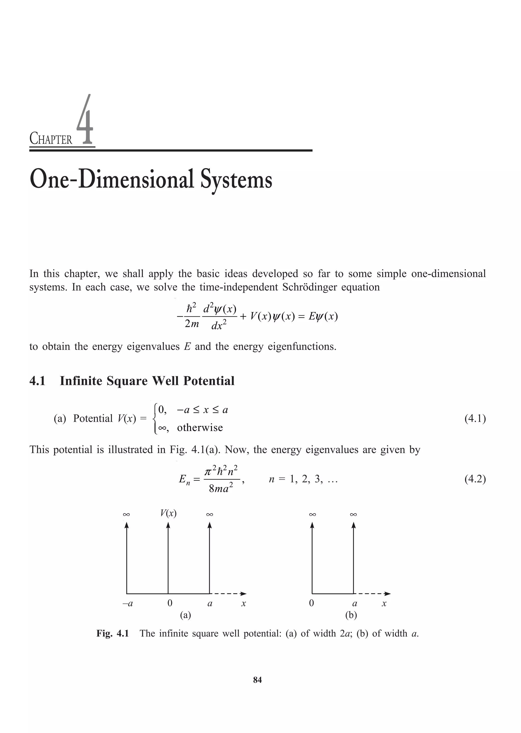
96. 86 ∑ Quantum Mechanics: 500 Problems with Solutions
Case (ii): E V0. In this case, the particle is not bound and the wave function is sinusoidal in all
the regions.
4.3 Square Potential Barrier
The potential is defined by
V(x) = V0 for 0 x a (4.11)
V(x) = 0, otherwise
Consider a stream of particles of mass m, the energy E V0 approaching the square barrier from the
left. A portion of the particles is reflected back and the rest is transmitted. For a broad high barrier,
the transmission coefficient T is given by
2
2 2 2
0
2 2 2 2
0
16 ( )
16
( )
a
a
a
a
-
-
-
= =
+
a
a
E V E e
k e
T
k V
(4.12)
where k and a have the same definitions as in Eq. (4.9).
4.4 Linear Harmonic Oscillator
4.4.1 The Schrödinger Method
The solution of the Schrödinger equation for the linear harmonic oscillator potential V = (1/2)kx2
,
where k = mw2
, gives the energy eigenvalues
1 1
,
2 2
n w
Ê ˆ Ê ˆ
= + = +
Á ˜ Á ˜
Ë ¯ Ë ¯
n
E n h n n = 0, 1, 2, º (4.13)
The normalized eigenfunctions are
2
1/2
/2
( ) ( )
2 !
y
n n
n
y H y e
n
a
y
p
-
Ê ˆ
= Á ˜
Ë ¯
(4.14)
where
y = ax and a =
1/2
mw
Ê ˆ
Á ˜
Ë ¯
(4.15)
y0(x) =
1/2 2 2
exp
2
x
a a
p
Ê ˆ
Ê ˆ
-
Á ˜
Á ˜
Ë ¯ Ë ¯
(4.16)
y1(x) =
1/2 2 2
(2 ) exp
2
2
x
x
a a
a
p
Ê ˆ
Ê ˆ
-
Á ˜
Á ˜
Ë ¯ Ë ¯
(4.17)
4.4.2 The Operator Method
The operator method is based on the basic commutation relation [x, p] = i, where x and p are the
coordinate and momentum operators. The creation (a†
) and annihilation (a) operators are defined by

97. One-Dimensional Systems ∑ 87
a†
=
1/2 1/2
1
2 2
m
x i p
m
w
w
Ê ˆ Ê ˆ
-
Á ˜ Á ˜
Ë ¯ Ë ¯
(4.18)
a =
1/2 1/2
1
2 2
m
x i p
m
w
w
Ê ˆ Ê ˆ
+
Á ˜ Á ˜
Ë ¯ Ë ¯
(4.19)
In terms of a†
and a, the Hamiltonian of a linear harmonic oscillator
H =
2
w
(aa†
+ a†
a) (4.20)
Also, we have
1
a n n n
| Ò = | - Ò , †
1 1
a n n n
| Ò = + | + Ò (4.21)
With these concepts, one can easily get the energy eigenvalues of a linear harmonic oscillator.
4.5 The Free Particle
The free-particle Schrödinger equation
2
2
2
,
d
k
dx
y
y
= - 2
2
2mE
k =
(4.22)
has the solutions
y(x) = Aeikx
and y(x) = Ae–ikx
(4.23)
As the normalization in the usual sense is not possible, one has to do either box normalization or
delta function normalization, which are, respectively,
1
( ) ikx
x e
L
y = and
1
( )
2
ikx
x e
y
p
-
= (4.24)
where L is the size of the box.

98. 88 ∑ Quantum Mechanics: 500 Problems with Solutions
PROBLEMS
4.1 Obtain the energy eigenvalues and eigenfunctions of a particle trapped in the potential
V(x) = 0 for 0 £ x £ a and V(x) = • otherwise. Show that the wave functions for the different energy
levels of the particle trapped in the square well are orthogonal.
Solution. The Schrödinger equation is
2 2
2
( )
( ) ( ),
2
d x
V x E x
m dx
y
y y
- + =
0 £ x £ a
2
2
2
( )
( ),
d x
k x
dx
y
y
= - 2
2
2mE
k =
y(x) = A sin kx + B cos kx, 0 £ x £ a
y(0) = 0 gives B = 0 or y (x) = A sin kx
y(a) = 0 gives A sin ka = 0 or sin ka = 0
ka = np or
2 2 2
2
,
2
n
n
E
ma
p
=
n = 1, 2, º
( ) 2/ sin
n x
x a
a
p
y =
0
*
a
i n dx
y y
Ú =
0
2
sin sin
a
m x n x
dx
a a a
p p
Ú
=
0
2
sin sin ,
x
ny my dy y
a
p
p
p
=
Ú
=
0
1
[cos ( ) cos ( ) ] 0
n m y n m y dy
p
p
- - + =
Ú
4.2 Consider a particle of mass m moving in a one dimensional potential specified by
0, 2 2
( )
, otherwise
a x a
V x
-
Ï
= Ì
•
Ô
Ó
Find the energy eigenvalues and eigenfunctions.
Solution. The time-independent Schrödinger equation for the region –2a x 2a (Fig. 4.2) is
2
2
2
0,
d
k
dx
y
y
+ = 2
2
2mE
k =
V(x)
• •
–2a 0 2a
Fig. 4.2 Infinite square well of bottom.

99. One-Dimensional Systems ∑ 89
Its solution is
y(x) = A sin kx + B cos kx
At x = ±2a, V(x) = •. Hence, y(±2a) = 0.
Application of this boundary condition gives
A sin (2ka) + B cos (2ka) = 0
–A sin (2ka) + B cos (2ka) = 0
From the above two relations,
A sin (2ka) = 0, B cos (2ka) = 0
Now, two possibilities arise: A = 0, B π 0 and A π 0, B = 0.
The first condition gives
cos (2ka) = 0; 2ka = ,
2
np
n = 1, 3, 5, º
k2
=
2 2
2 2
2
16
n
mE
n
a
p
=
En =
2 2 2
2
,
32
n
ma
p
n = 1, 3, 5, º
yn = cos ,
4
n x
B
a
p
n = 1, 3, 5, º
Normalization yields
1
cos ,
4
2
n
n x
a
a
p
y = n = 1, 3, 5, º
The condition A π 0, B = 0 leads to
En =
2 2 2
2
,
32
n
ma
p
n = 2, 4, 6, º
1
sin ,
4
2
n
n x
a
a
p
y = n = 2, 4, 6, º
4.3 For an electron in a one-dimensional infinite potential well of width 1 Å, calculate (i) the
separation between the two lowest energy levels; (ii) the frequency and wavelength of the photon
corresponding to a transition between these two levels; and (iii) in what region of the electromagnetic
spectrum is this frequency/wavelength?
Solution.
(i) From Eq. (4.2),
En =
2 2 2
2
,
8
n
ma
p
2a = 1 Å = 10–10
m
E2 – E1 =
2 2 2 34 2
2 31 20 2
3 3 (1.055 10 J s) 4
8 8(9.1 10 kg) 10 m
ma
p p -
- -
¥ ¥ ¥ ¥
=
¥
= 1.812 ¥ 10–17
J = 113.27 eV

100. 90 ∑ Quantum Mechanics: 500 Problems with Solutions
(ii) hn = 1.812 ¥ 10–17
J
n = 2.7 ¥ 1016
8 1
8
16 1
3 10 ms
1.1 10 m
2.7 10 s
c
l
n
-
-
-
¥
= = = ¥
¥
(iii) This frequency falls in the vacuum ultraviolet region.
4.4 Show that the energy and the wave function of a particle in a square well of finite depth V0
reduces to the energy and the wave function of a square well with rigid walls in the limit V0 Æ •.
Solution. For a well of finite depth V0, Eq. (4.7) gives
tan ka = ,
k
a 2
2
2
,
mE
k =
2
0
2
2
( )
m
V E
a = -
tan ka = 0
V E
E
-
or
0
Lt tan
V
ka
Æ•
Æ •
ka =
2
np
or k2
a2
=
2 2
4
n p
En =
2 2 2
2
8
n
ma
p
[which is the same as Eq. (4.2).]
The wave functions in the different regions will be
,
( ) sin cos ,
,
x
x
Ae x a
x B kx C kx a x a
De x a
a
a
y
-
Ï -
Ô
= + -
Ì
Ô
Ô
Ó
When V0 Æ •, a Æ •, and the wave function reduces to
0,
( ) sin cos ,
0,
x a
x A kx B kx a x a
x a
y
-
Ï
Ô
= + -
Ì
Ô
Ó
which is the wave function of a particle in a square well with rigid walls.
4.5 Calculate the expectation values of position ·xÒ and of the momentum ·pxÒ of the particle
trapped in the one-dimensional box of Problem 4.1.
Solution.
·xÒ =
0
2
sin sin
a
n x n x
x dx
a a a
p p
Ú
=
2
0 0
2 1 2
sin 1 cos
a a
n x n x
x dx x dx
a a a a
p p
Ê ˆ
= -
Á ˜
Ë ¯
Ú Ú
=
0 0
1 1 2
cos
a a
n x
x dx x dx
a a a
p
-
Ú Ú

101. One-Dimensional Systems ∑ 91
As the second term vanishes when integrated by parts,
·xÒ =
2
a
·pxÒ =
0
2
sin sin
a
n x d n x
i dx
a a dx a
p p
Ê ˆ
-
Á ˜
Ë ¯
Ú
= 2
0
2
sin cos
a
n n x n x
i dx
a a
a
p p p
- Ú
= 2
0
2
sin 0
a
n nx
i dx
a
a
p p
- =
Ú
4.6 An electron in a one-dimensional infinite potential well, defined by V(x) = 0 for –a £ x £ a
and V(x) = • otherwise, goes from the n = 4 to the n = 2 level. The frequency of the emitted photon
is 3.43 ¥ 1014
Hz. Find the width of the box.
Solution.
2 2 2
2
,
8
n
n
E
ma
p
=
m = 9.1 ¥ 10–31
kg
E4 – E2 =
2 2
2
12
8
h
ma
p
n
=
a2
=
34
31 14 1
3 3(6,626 10 J s)
8 8(9.1 10 kg)(3.43 10 s )
h
mn
-
- -
¥
=
¥ ¥
= 79.6 ¥ 10–20
m2
a = 8.92 ¥ 10–10
m or 2a = 17.84 ¥ 10–10
m
4.7 A particle of mass m trapped in the potential V(x) = 0 for –a £ x £ a and V(x) = • otherwise.
Evaluate the probability of finding the trapped particle between x = 0 and x = a/n when it is in the
nth state.
Solution. Wave function y(x) =
2
sin
n x
a a
p
(refer Problem 1)
Probability density P(x) = 2
2
sin
n x
a a
p
Required probability P =
/ /
2
0 0
2
( ) sin
a n a n
n x
P x dx dx
a a
p
=
Ú Ú
P =
/
0
1 2 1
1 cos
a n
n x
dx
a a n
p
Ê ˆ
- =
Á ˜
Ë ¯
Ú

102. 92 ∑ Quantum Mechanics: 500 Problems with Solutions
4.8 An alpha particle is trapped in a nucleus of radius 1.4 ¥ 10–15
m. What is the probability that
it will escape from the nucleus if its energy is 2 MeV? The potential barrier at the surface of the
nucleus is 4 MeV and the mass of the a-particle = 6.64 ¥ 10–27
kg.
Solution. Transmission coefficient T = 0
0 0
2
16 1 exp 2 ( )
E e a
m V E
V V
Ê ˆ È ˘
- - -
Á ˜ Í ˙
Ë ¯ Î ˚
Mass of alpha particle = 6.64 ¥ 10–27
kg
0
2 ( )
m V E
- = 27 6 19 1/2
[2(6.64 10 kg)(2 10 eV) (1.6 10 J/eV)]
- -
¥ ¥ ¥
= 6.52 ¥ 10–20
kg m s–1
0
2
2 ( )
a
m V E
-
=
15
20 1
34
2(2.8 10 m)
6.52 10 kg ms 3.477
1.05 10 J s
-
- -
-
¥
¥ ¥ =
¥
T =
1 1
16 exp ( 3.477) 0.124
2 2
¥ ¥ ¥ - =
4.9 The wave function of a particle confined in a box of length a is
2
( ) sin ,
x
x
a a
p
y = 0 £ x £ a
Calculate the probability of finding the particle in the region 0 x a/2.
Solution. The required probability P =
/2
2
0
2
sin
a
x
dx
a a
p
Ú
=
/2
0
1 2
1 cos
a
x
dx
a a
p
Ê ˆ
-
Á ˜
Ë ¯
Ú
=
/2 /2
0 0
1 1 2 1
cos
2
a a
x
dx dx
a a a
p
- =
Ú Ú
4.10 Find ·xÒ and ·pÒ for the nth state of the linear harmonic oscillator.
Solution. For the harmonic oscillator, yn(x) = AHn(x) exp (–mwx2
/2)
2
2 2
( ) exp 0
n
m x
x A H x x dx
w
•
-•
Ê ˆ
· Ò = - =
Á ˜
Ë ¯
Ú
since the integrand is an odd function of x.
·pÒ =
2 2
2
( ) exp exp
2 2
n n
m x d m x
i A H x H dx
dx
w w
•
-•
È ˘
Ê ˆ Ê ˆ
- - -
Í ˙
Á ˜ Á ˜
Ë ¯ Ë ¯
Í ˙
Î ˚
Ú
=
2 2
2 2
exp exp
n n n
m x m x m x
i A H H H dx
w w w
•
-•
È ˘
Ê ˆ Ê ˆ
- - - -
Í ˙
Á ˜ Á ˜
Ë ¯ Ë ¯
Í ˙
Î ˚
Ú
= 0
since both the integrand terms are odd functions of x. Here, H¢n = dHn/dx.

103. One-Dimensional Systems ∑ 93
4.11 For the nth state of the linear harmonic oscillator, evaluate the uncertainty product (Dx) (Dp).
Solution. According to the Virial theorem, the average values of the kinetic and potential energies
of a classical harmonic oscillator are equal. Assuming that this holds for the expectation values of
the quantum oscillator, we have
2 2
1 1 1
2 2 2 2
x
p k x n
m
w Ê ˆ
· Ò = · Ò = +
Á ˜
Ë ¯
k = mw2
Hence,
2 1
2
x
p m n
w
Ê ˆ
· Ò = +
Á ˜
Ë ¯
,
2 1
2
x n
mw
Ê ˆ
· Ò = +
Á ˜
Ë ¯
2 2 2 2
( )
x x x x
D = · Ò - · Ò = · Ò [refer Problem 4.10]
(Dpx)2
= 2
x
p
· Ò
2
2 2 2
1
( ) ( ) ,
2
x
x p n
Ê ˆ
D D = +
Á ˜
Ë ¯
1
( )( )
2
x
x p n
Ê ˆ
D D = +
Á ˜
Ë ¯
4.12 A harmonic oscillator is in the ground state. (i) Where is the probability density maximum?
(ii) What is the value of maximum probability density?
Solution.
(i) The ground state wave function
1/4 2
0 ( ) exp
2
m m x
x
w w
y
p
Ê ˆ
-
Ê ˆ
= Á ˜ Á ˜
Ë ¯ Ë ¯
The probability density
P(x) =
1/2 2 2
0 0
* exp
m m x
w w
y y
p
Ê ˆ
Ê ˆ
= -
Á ˜ Á ˜
Ë ¯ Ë ¯
P(x) will be maximum at the point where
1/2 2 2
0 2 exp
dP m m m x
x
dx
w w w
p
Ê ˆ
Ê ˆ Ê ˆ
= = - -
Á ˜ Á ˜ Á ˜
Ë ¯ Ë ¯ Ë ¯
x = 0
Thus, the probability density is maximum at x = 0.
(ii) P(0) =
1/2
mw
p
Ê ˆ
Á ˜
Ë ¯
4.13 A 1 eV electron got trapped inside the surface of a metal. If the potential barrier is 4.0 eV
and the width of the barrier is 2 Å, calculate the probability of its transmission.
Solution. If L is the width of the barrier, the transmission coefficient
T =
2
16 1 exp 2 ( )
E E L
m V E
V V
Ê ˆ È ˘
- - -
Á ˜ Í ˙
Ë ¯ Î ˚
=
10
31 19
34
1 3 2 2 10 m
16 exp 2(9.1 10 kg)(3 1.6 10 J)
4 4 1.05 10 J s
-
- -
-
Ê ˆ
¥ ¥
¥ ¥ ¥ - ¥ ¥ ¥
Á ˜
¥
Ë ¯
= 0.085

104. 94 ∑ Quantum Mechanics: 500 Problems with Solutions
4.14 An electron is in the ground state of a one-dimensional infinite square well with a = 10–10
m.
Compute the force that the electron exerts on the wall during an impact on either wall.
Solution. The force on the wall
F = n
dE
da
-
The energy of the ground state
2 2
1 2
2
E
ma
p
=
and hence the force on the wall
F =
10 10
2 2
1
3
10 10
a a
dE
da ma
p
- -
= =
- =
=
2 34 2
31 10 3
(1.054 10 J s)
(9.1 10 kg)(10 m)
p -
- -
¥
¥
= 1.21 ¥ 10–7
N
4.15 Show that the probability density of the linear harmonic oscillator in an arbitrary superposition
state is periodic with the period equal to the period of the oscillator.
Solution. The time-dependent wave function of the linear harmonic oscillator in a superposition
state is
( , ) ( ) exp( / )
n n n
n
x t C x iE t
y
Y = -
Â
where yn(x) is the time-independent wave function of the harmonic oscillator in the nth state. The
probability density
2
* *
( , ) ( , ) exp[ ( ) / )]
m n m n m n
m n
P x t x t C C i E E t
y y
= |Y | = -
ÂÂ
It is obvious that P(x, t) is dependent on time. Let us investigate what happens to P(x, t) if t is
replaced by t + 2p/w. It follows that
( ) 2
exp m n
i E E
t
p
w
È ˘
- Ê ˆ
+
Í ˙
Á ˜
Ë ¯
Î ˚
=
( ) ( ) 2
exp exp
m n m n
i E E t i E E p
w
- -
È ˘ È ˘
Í ˙ Í ˙
Î ˚ Î ˚
=
( )
exp m n
i E E t
-
È ˘
Í ˙
Î ˚
since (Em – En) is an integral multiple of w, i.e., P(x, t) is periodic with period 2p/w, the period of
the linear harmonic oscillator.
4.16 For harmonic oscillator wave functions, find the value of (yk, xyn).
Solution. For Hermite polynomials,
Hn+1(y) – 2yHn(y) + 2nHn–1(y) = 0

105. One-Dimensional Systems ∑ 95
Substituting the values of Hn+1, Hn and Hn-1 in terms of the oscillator wave functions, [(Eq. 4.14)],
and dropping
2
/2 1/4
( / )
y
e m
p w
from all terms, we get
1 1/2 1/2 1 1/2
1 1
[2 ( 1)!] 2 (2 !) 2 [2 ( 1)!] 0
n n n
n n n
n y n n n
y y y
+ -
+ -
+ - + - =
1/2 1/2
1 1
( 1)] 2 0
n n n
n y n
y y y
+ -
+ - + =
Since y = (mw/)1/2
x, the inner product of this equation with yk gives
1/2 1/2 1/2
1 1
( 1) ( , ) (2 / ) ( , ) ( , ) 0
k n k n k n
n m x n
y y w y y y y
+ -
+ - + =
1/2 1/2
1 1
( 1)
( , ) ( , ) ( , )
2 2
k n k n k n
n n
m m
y y y y y y
w w
+ -
+
È ˘ Ê ˆ
= + Á ˜
Í ˙ Ë ¯
Î ˚
(yk, xyn) =
( 1)/2 if = + 1
/2 if = – 1
0 if 1
n m k n
n m k n
k n
w
w
Ï +
Ô
Ô
Ì
Ô π ±
Ô
Ó
4.17 Evaluate ·x2
Ò, ·p2
Ò, ·VÒ and ·TÒ for the states of a harmonic oscillator.
Solution. From Problem 4.16,
1/2
1/2 1/2
1 1
2
( 1) 0
n n n
m
n x n
w
y y y
+ -
Ê ˆ
+ - + =
Á ˜
Ë ¯
Multiplying from left by x and then taking the inner product of the resulting equation with yn, we
get
1/2
1/2 2 1/ 2
1 1
2
( 1) ( , ) ( , ) ( , ) 0
n n n n n n
m
n x x n x
w
y y y y y y
+ -
Ê ˆ
+ - + =
Á ˜
Ë ¯
Using the results of Problem 4.16, we obtain
2
( 1) 2
1 ( , ) 0
2 2
n n
n m n
n x n
m m
w
y y
w w
+
+ - + =
2
2
(2 1) ( , )
2 n n
n m
n x
m
w
y y
w
+ =
·x2
Ò = 2
( , ) (2 1)
2
n n
x n
m
y y
w
= +
·p2
Ò =
2
2
2
, n
n
d
dx
y
y
Ê ˆ
- Á ˜
Ë ¯
The Schrödinger equation for harmonic oscillator is
2 2 2 2
2 2 2
2
n n
n n
d mE m x
dx
y w
y y
= - +

106. 96 ∑ Quantum Mechanics: 500 Problems with Solutions
Substituting this value of d2
yn/dx2
and using the result for ·x2
Ò, we get
·p2
Ò = 2 2 2
2 ( , ) ( , )
n n n n n
mE m x
y y w y y
-
·p2
Ò = 2 2
2 (2 1)
2
n
mE m n
m
w
w
- +
=
(2 1)
(2 1)
2
n
n m m
w w
+
+ -
=
(2 1) 1
2 2
n
m m n
w w
+ Ê ˆ
= +
Á ˜
Ë ¯
Expectation value of potential energy = 2
1
2
k x
· Ò
·VÒ =
1 1
2 2 2
n
E
n w
Ê ˆ
+ =
Á ˜
Ë ¯
The expectation value of kinetic energy
·T Ò = 2
1 1 1
2 2 2 2
n
E
p n
m
w
Ê ˆ
· Ò = + =
Á ˜
Ë ¯
4.18 Show that the zero point energy of (1/2) w of a linear harmonic oscillator is a manifestation
of the uncertainty principle.
Solution. The average position and momentum of a classical harmonic oscillator bound to the
origin is zero. According to Ehrenfest’s theorem, this rule must be true for the quantum mechanical
case also. Hence,
(Dx)2
= ·x2
Ò – ·xÒ2
= ·x2
Ò
(Dp)2
= ·p2
Ò – ·pÒ2
= ·p2
Ò
For the total energy E,
·EÒ = 2 2
1 1
,
2 2
p k x
m
· Ò + · Ò k = mw2
= 2 2
1 1
2 2
p k x
m
·D Ò + ·D Ò
Replacing ·DpÒ2
with the help of the relation
·DpÒ2
·DxÒ2
≥
2
4
·EÒ ≥
2
2
2
1
2
8 ( )
k x
m x
+ ·D Ò
D
For the RHS to be minimum, the differential of ·EÒ with respect to ·DxÒ2
must be zero, i.e.,
2
4
min
1
0
2
8 ( )
k
m x
+ =
D
or
2
2
min
( )
2
x
mw
D =
2
2
min
2 1 1
8 2 2 2
m
E m
m m
w
w w
w
· Ò = + =

107. One-Dimensional Systems ∑ 97
4.19 A stream of particles of mass m and energy E move towards the potential step V(x) = 0 for
x 0 and V(x) = V0 for x 0. If the energy of the particles E V0, show that the sum of fluxes
of the transmitted and reflected particles is equal to the flux of incident paricles.
Solution. The Schrödinger equation for regions 1 and 2 (see Fig. 4.3) are
2
2
1
0
2
0,
d
k
dx
y
y
+ = 2
0 2
2
,
mE
k =
x 0
2
2
2
2
0,
d
k
dx
y
y
+ = 2 0
2
2 ( )
,
m E V
k
-
=
x 0
The solutions of the two equations are
0 0
1 ,
ik x ik x
e Ae
y -
= + x 0
2 ,
ikx
Be
y = x 0
For convenience, the amplitude of the incident wave is taken as 1. The second term in y1, a wave
travelling from right to left, is the reflected wave whereas y2 is the transmitted wave. It may be noted
that in region 2 we will not have a wave travelling from right to left. The continuity conditions on
y and its derivative at x = 0 give
1 + A = B, k0 (1 – A) = kB
Simplifying, we get
A = 0
0
,
k k
k k
-
+
B = 0
0
2k
k k
+
Flux of particles for the incident wave (see Problem 2.22) = 0
k
m
Magnitude of flux of particles for the reflected wave = 0
k
m
|A|2
Flux of particles for the transmitted wave =
k
m
|B|2
The sum of reflected and transmitted flux is given by
2
2 2 0 0 0 0
0 2 2
0 0
( ) 4
[ ]
( ) ( )
k k k kk k
k A k B
m m m
k k k k
È ˘
-
| | + | | = + =
Í ˙
+ +
Í ˙
Î ˚
which is the incident flux.
Fig. 4.3 Potential step.
E
V = V0
V = 0
Region 1 Region 2
0 x

108. 98 ∑ Quantum Mechanics: 500 Problems with Solutions
4.20 A stream of particles of mass m and energy E move towards the potential step of
Problem 4.19. If the energy of particles E V0, show that there is a finite probability of finding the
particles in the region x 0. Also, determine the flux of (i) incident particles, (ii) reflected particles,
and (iii) the particles in region 2. Comment on the results.
Solution. The Schrödinger equation and its solution for the two regions (see Fig. 4.3) are
2
2
1
0 1
2
0,
d
k
dx
y
y
+ = 2
0 2
2
,
mE
k =
x 0
2
2
2
2
2
0,
d
dx
y
g y
- = 2 0
2
2 ( )
,
m V E
g
-
=
x 0
y1 = 0 0
,
ik x ik x
e Be-
+ x 0
y2 = Ce–gx
, x 0
The solution eg x
in region 2 is left out as it diverges and the region is an extended one. The continuity
condition at x = 0 gives
1 + B = C, ik0 (1 – B) = –g C
Solving, we get
B = 0
0
,
ik
ik
g
g
+
-
C = 0
0
2ik
ik g
-
The reflection coefficient
R = | B |2
=
0 0
0 0
1
ik ik
ik ik
g g
g g
+ - +
Ê ˆ Ê ˆ
=
Á ˜ Á ˜
- - -
Ë ¯ Ë ¯
Reflected flux = 2
0 0
k k
B
m m
- | | = -
The negative sign indicates that it is from right to left. Since y2 is real, the transmitted flux = 0
and, therefore, the transmission coefficient T = 0. However, the wave function in the region x 0
is given by
0
2
0
2 x
ik
e
ik
g
y
g
-
=
-
Therefore, the probability that the particle is found in the region x 0 is finite. Due to the uncertainty
in energy, the total energy may even be above V0.
4.21 A beam of 12 eV electrons is incident on a potential barrier of height 30 eV and width
0.05 nm. Calculate the transmission coefficient.
Solution. The transmission coefficient T is given by
0
0
2
0
16 ( ) 2
exp 2 ( )
E V E a
T m V E
V
- È ˘
= - -
Í ˙
Î ˚
0
2
0
16 ( ) 16 12 18
3.84
30 30
E V E
V
- ¥ ¥
= =
¥

109. One-Dimensional Systems ∑ 99
0
2
2 ( )
a
m V E
-
=
9
31 19 1/2
34
2(0.05 10 m)
2 (9.1 10 kg)(18 1.6 10 J)
(1.054 10 J s)
-
- -
-
¥
¥ ¥ ¥ ¥ ¥
¥
= 2.172
T =
3.84 3.84
0.44
exp (2.172) 8.776
= =
4.22 For the nth state of the linear harmonic oscillator, what range of x values is allowed
classically? In its ground state, show that the probability of finding the particle outside the classical
limits is about 16 per cent.
Solution. At the classical turning points, the oscillator has only potential energy. Hence, at the
turning points,
2 2
1 1
2 2
m x n
w w
Ê ˆ
= +
Á ˜
Ë ¯
1/2
(2 1)
n
x
mw
+
È ˘
= ± Í ˙
Î ˚
The allowed range of x values are
1/2 1/2
(2 1) (2 1)
n n
x
m m
w w
+ +
È ˘ È ˘
-
Í ˙ Í ˙
Î ˚ Î ˚
When the oscillator is in the ground state, the turning points are
1/2
mw
Ê ˆ
- Á ˜
Ë ¯
and
1/2
mw
Ê ˆ
Á ˜
Ë ¯
The ground state wave function is
1/4 2
0( ) exp
2
m m x
x
w w
y
p
Ê ˆ
Ê ˆ
= -
Á ˜ Á ˜
Ë ¯ Ë ¯
The probability for the particle to be outside, the classical limits are
P =
1/2 1/2
1/2 2
2
0
( / ) ( / )
2 2 exp
m m
m m x
dx dx
w w
w w
y
p
• • Ê ˆ
Ê ˆ
| | = -
Á ˜ Á ˜
Ë ¯ Ë ¯
Ú Ú
=
2
1/2 1/2
1
2 2
0.1418 0.1599 16%
y
e dy
p p
•
-
= ¥ = =
Ú
4.23 An electron moves in a one-dimensional potential of width 8 Å and depth 12 eV. Find the
number of bound states present.
Solution. If follows from Eq. (4.10) that, if the width is 2a, Then
(a) One bound state exists if 0 V0a2
p2
2
/8m.
(b) Two bound states exist if p2
2
/8m V0a2
4p2
2
/8m.
(c) Three bound states exist if 4p2
2
/8m V0a2
9p2
2
/8m.
(d) Four bound states exist if 9p2
2
/8m V0a2
16p2
2
/8m, º

110. 100 ∑ Quantum Mechanics: 500 Problems with Solutions
In the given case, the width is 8Å, and hence a = 4Å = 4 ¥ 10–10
m. Therefore,
V0a2
= (12 ¥ 1.6 ¥ 10–19
J) (16 ¥ 10–20
m2
) = 307.2 ¥ 10–39
kg m4
s–2
2 2 2 34 2
39 4 2
31
(1.05 10 J s)
14.96 10 kg m s
8m 8(9.1 10 kg)
p p -
- -
-
¥
= = ¥
¥
V0a2
= 307.2 ¥ 10–39
kg m4
s–2
lies between
2 2
16
8m
p
and
2 2
25
8 m
p
Thus, the number of bound states present is 5.
4.24 A linear harmonic oscillator is in the first excited state. (i) At what point is its probability
density maximum? (ii) What is the value of maximum probability density?
Solution. The harmonic oscillator wave function in the n = 1 state is
1/2 2 2
1( ) 2 exp
2
2
a x
x x
a
y a
p
Ê ˆ
Ê ˆ -
= Á ˜
Á ˜
Ë ¯ Ë ¯
1/2
mw
a
Ê ˆ
= Á ˜
Ë ¯
(i) Probability density P(x) =
3
2 2 2
2
* exp ( )
x x
a
yy a
p
= -
P(x) is maximum when dP/dx = 0, and hence
3
2 3
2
0 (2 2 )
x x
a
a
p
= - or
1
x
a
= ±
(ii) Maximum value of P(x) =
2 1 2 1
0.415
2.718
e
a a
a
p p
= =
4.25 Sketch the probability density |y|2
of the linear harmonic oscillator as a function of x for
n = 10. Compare the result with that of the classical oscillator of the same total energy and discuss
the limit n Æ •.
Solution. Figure 4.4 illustrates the probability | y10 |2
(n = 10: solid curve). For n = 0, the
probability is maximum at x = 0. As the quantum number increases, the maximum probability moves
towards the extreme positions. This can be seen from the figure. For a classical oscillator, the
probability of finding the oscillator at a given point is inversely proportional to it s velocity at that
point. The total energy
2 2
1 1
2 2
E m kx
= +
v or
2
2E kx
m
-
=
v
Therefore, the classical probability
2
2
c
m
P
E kx
µ
-
This is minimum at x = 0 and maximum at the extreme positions. Figure 4.4 also shows the classical
probability distribution (dotted line) for the same energy. Though the two distributions become more
and more similar for high quantum numbers, the rapid oscillations of |y10 |2
is still a discrepancy.

111. One-Dimensional Systems ∑ 101
4.26 Calculate the energy levels and wave functions of a particle of mass m moving in the one-
dimensional potential well defined by
2 2
for 0
( ) 1
for 0
2
x
V x
m x x
w
•
Ï
Ô
= Ì
Ô
Ó
Solution. The harmonic oscillator wave function is given by Eq. (4.14). As H1(x), H3(x), H5(x)º
are zero at x = 0, y(0) = 0 for odd quantum numbers. However, for n = 0, 2, 4, º, y(0) π 0, but
finite. The given potential is the same as the simple harmonic oscillator for x 0 and V(x) = • for
x 0. Hence, y(0) has to be zero. Therefore, the even quantum number solutions are not physically
acceptable. Consequently, the energy eigenvalues and eigenfunctions are the same as the simple
harmonic oscillators with n = 1, 3, 5, º
4.27 The strongest IR absorption band of 12
C16
O molecule occurs at 6.43 ¥ 1013
Hz. If the reduced
mass of 12
C16
O is 1.385 ¥ 10–26
kg, calculate (i) the approximate zero point energy, and (ii) the force
constant of the CO bond.
Solution. Zero point energy e0 = (1/2)hv0, and hence
e0 = 34 13 1
1
(6.626 10 J s) (6.43 10 s )
2
- -
¥ ¥
= 21.30 ¥ 10–21
J = 0.133 eV
The force constant k = 2 2
0
4 ,
p n m and therefore,
k = 4p2
¥ (6.43 ¥ 1013
s–1
)2
(1.1385 ¥ 10–26
kg)
= 1860 N m–1
Fig. 4.4 The probability density |y |2
for the state n = 10 (solid curve) and for a classical oscillator of the same
total energy (broken curve).

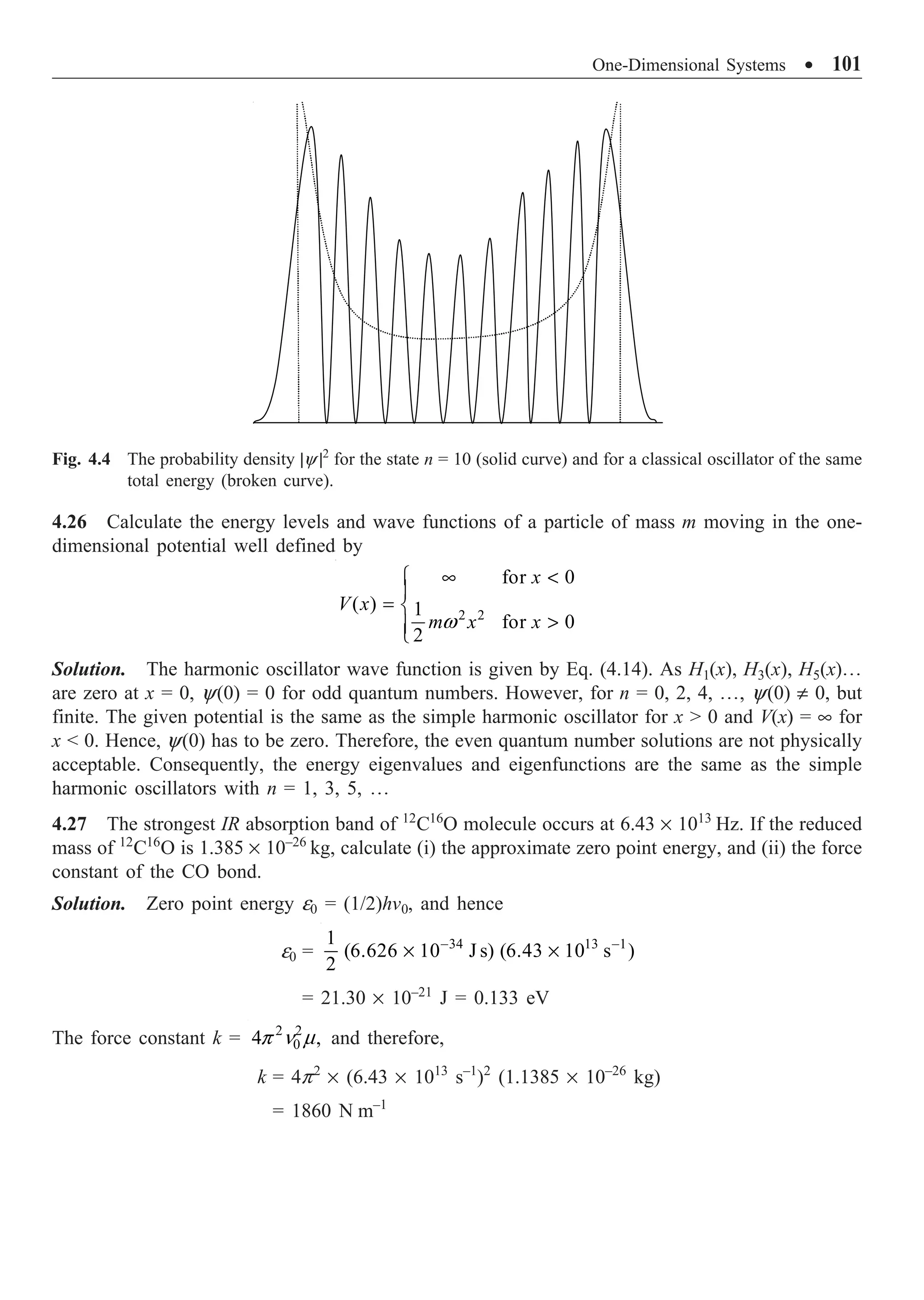
112. 102 ∑ Quantum Mechanics: 500 Problems with Solutions
4.28 A particle of mass m confined to move in a potential V(x) = 0 for 0 £ x £ a and V(x) = •
otherwise. The wave function of the particle at time t = 0 is given by
5 2
( ,0) sin cos
x x
x A
a a
p p
y =
(i) Normalize y(x, 0), (ii) Find y(x, t), (iii) Is y(x, t) a stationary state?
Solution. Given
5 2 7 3
( ,0) sin cos sin sin
2
x x A x x
x A
a a a a
p p p p
y
Ê ˆ
= = +
Á ˜
Ë ¯
(i) The normalization condition gives
2
2
0
7 3
sin sin
4
a
A x x
dx
a a
p p
Ê ˆ
+
Á ˜
Ë ¯
Ú = 1
2
2 2
0
7 3 7 3
sin sin 2 sin sin
4
a
A x x x x
dx
a a a a
p p p p
Ê ˆ
+ +
Á ˜
Ë ¯
Ú = 1
2
1
4 2 2
A a a
Ê ˆ
+ =
Á ˜
Ë ¯
or
2
A
a
=
Normalized y(x, 0) is
1 7 3
( , 0) sin sin
x x
x
a a
a
p p
y
Ê ˆ
= +
Á ˜
Ë ¯
For a particle in an infinite square well, the eigenvalues and eigenfunctions are
2 2 2
2
,
2
n
n
E
ma
p
=
1/2
2
( ) sin ,
n
n x
x
a a
p
f
Ê ˆ
= Á ˜
Ë ¯
n = 1, 2, 3, º
Hence,
7 3
1 1 7 3
( , 0) ( ) sin sin
2
x x
x
a a
a
p p
y f f
Ê ˆ
= + = +
Á ˜
Ë ¯
(ii) The time dependence of a state is given by
y(x, t) = y(x, 0) e (–iEt/)
Hence, y(x, t) in this case is
7 7 3 3
1
( , ) [ exp ( / ) exp ( / )]
2
x t iE t iE t
y f f
= - + -
(iii) It is not a stationary state since y(x, t) is a superposition state.
4.29 Consider a particle of mass m in the one-dimensional short range potential
V(x) = –V0d(x), V0 0
where d (x) is the Dirac delta function. Find the energy of the system.

113. One-Dimensional Systems ∑ 103
Solution. The Schrödinger equation for such a potential is
2 2
0
2
( )
( ) ( ) ( )
2
d x
V x x E x
m dx
y
d y y
- - =
2
0
2 2 2
2
2
( )
mV
d mE
x
dx
y y
d y
+ = -
Since the potential is attractive, when E 0, the equation to be solved is
2
2 0
2 2
2
( )
mV
d
k x
dx
y
y d y
- = -
, 2
2
2m E
k
| |
=
The solution everywhere except at x = 0 must satisfy the equation
2
2
2
0
d
k
dx
y
y
- =
and for the solution to vanish at x Æ ±•, we must have
, 0
( )
, 0
kx
kx
e x
x
e x
y
-
Ï
Ô
= Ì
Ô
Ó
(i)
The normalization factor is assumed to be unity. Integrating the original equation from –l to +l, l
being an arbitrarily small positive number, we get
2 0
2
2
( ) ( )
mV
d
k dx x x dx
dx
l l l
l l l
y
y d y
- - -
Ê ˆ
- = -
Á ˜
Ë ¯ Ú Ú
The integral on the RHS becomes –(2mV0/2) y(0) (refer the Appendix). Hence, in the limit
l Æ 0, the above equation becomes
0
2
0 0
2
(0)
x x
mV
d d
dx dx
y y
y
= + = -
Ê ˆ Ê ˆ
- = -
Á ˜ Á ˜
Ë ¯ Ë ¯
Substituting the values of the LHS from Eq. (i), we get
0
2
2
(0) (0) (0)
mV
k k
y y y
- - = -
0
2
mV
k =
or
2 2
0
2 4
2 m V
m E
| |
=
2
0
2
2
mV
E
| | =
or
2
0
2
2
mV
E = -
4.30 Consider the one-dimensional problem of a particle of mass
m in a potential V = • for x 0; V = 0 for 0 £ x £ a, and V = V0
for x a (see Fig. 4.5). Obtain the wave functions and show that
the bound state energies (E V0) are given by
0
2
tan
mE E
a
V E
= -
-
Fig. 4.5 Potential defined in
Problem 4.30.
•
V(x) V0
0 a x

114. 104 ∑ Quantum Mechanics: 500 Problems with Solutions
Solution. The Schrödinger equation for the different regions are
2
2
2
0,
d
k
dx
y
y
+ = 2
2
2
,
mE
k =
0 £ x £ a
2
2
1
2
0,
d
k
dx
y
y
- = 2
1 0
2
2
( ),
m
k V E
= -
x a
The solution of these equations are
y = A sin kx + B cos kx, 0 £ x £ a
1 1
,
k x k x
Ce De
y -
= + x a
where A, B, C and D are constants. Applying the boundary conditions y = 0 at x = 0 and y Æ 0
as x Æ •, we get
y = A sin kx, 0 £ x £ a
y = 1
,
k x
Ce-
x 0
The requirement that y and dy/dx are continuous at x = a gives
A sin ka = 1
k a
Ce-
Ak cos ka = 1
1
k a
Ck e-
Dividing one by the other, we obtain
1
tan
k
ka
k
= -
1/2
0
2
tan
mEa E
V E
Ê ˆ Ê ˆ
= -
Á ˜ Á ˜
-
Ë ¯
Ë ¯
4.31 Consider a stream of particles of mass m, each moving in the positive x-direction with kinetic
energy E towards the potential barrier. Then,
V(x) = 0 for x £ 0
V(x) =
3
4
E
for x 0
Find the fraction of the particles reflected at x = 0.
Solution. The Schrödinger equations for the different regions are
2
2
2
0,
d
k
dx
y
y
+ = 2
2
2mE
k =
, x £ 0 (i)
2
2 2
2 3
0,
4
d m E
E
dx
y
y
Ê ˆ
- - =
Á ˜
Ë ¯
x 0
2
2
2
0,
2
d k
dx
y
y
Ê ˆ
+ =
Á ˜
Ë ¯
x 0 (ii)

115. One-Dimensional Systems ∑ 105
The solution of equation (i) is
y = eikx
+ re–ikx
, x £ 0
where r is the amplitude of the reflected wave since e–ikx
represents a wave travelling in the negative
x-direction. The solution of equation (ii) is
/2
,
ikx
te
y = x 0
where t is the amplitude of the transmitted wave. It is also oscillatory since the height of the barrier
is less than the kinetic energy of the particle. As the wave function is continuous at x = 0,
1 + r = t
Since the derivative dy/dx is continuous at x = 0,
(1 )
2
t
r
- =
Solving the two equations, r = 1/3 and hence one-ninth of the particle is reflected at x = 0.
4.32 An electron of mass m is contained in a cube of side a, which is fairly large. If it is in an
electromagnetic field characterized by the vector potential 0 ˆ ˆ
,
B xy y
=
A being the unit vector along
the y-axis, determine the energy levels and eigenfunctions.
Solution. The Hamiltonian operator of the electron having charge –e is
2
2 2
0
1
2 x y z
B ex
H p p p
m c
È ˘
Ê ˆ
Í ˙
= + + +
Á ˜
Ë ¯
Í ˙
Î ˚
where px, py, pz are operators. We can easily prove the following commutation relations:
[H, py] = [H, pz] = 0, [H, px] π 0
Hence, py and pz are constants. The Schrödinger equation is
2 2 2
2
0
2 2 2
0
2 2
2
1
2
y
y z
B ep x
B e x
d
p p E
m c
dx c
y y
Ê ˆ
- + + + + =
Á ˜
Ë ¯
2
2 2 2
2 2
0 2
0
2 2
1
2 2 2
2
y y
z
B ep x p
B e x
d
E p
m mc m m
dx mc
y
y y
Ê ˆ
- Ê ˆ
+ + + = -
Á ˜ Á ˜
Ë ¯
Ë ¯
we now introduce a new variable x1 defined by
1
0
y
cp
x x
B e
= +
2 2
2 2
1 2 2
0 0
2 y y
cp x c p
x x
B e B e
= + +
Multiplying by 2 2 2
0 /(2 )
B e mc , we get
2
2 2 2 2 2 2
0
0 1 0
2 2 2
2 2
y y
B ep x p
B e x B e x
mc m
mc mc
= + +

116. 106 ∑ Quantum Mechanics: 500 Problems with Solutions
In terms of the new variable, the Schrödinger equation takes the form
2 2 2
2 2
2
0 1
2 2
1
1 1
2 2 2 z
B e x
d
E p
m m
dx mc
y
y
y
Ê ˆ
- + = -
Á ˜
Ë ¯
The form of this equation is similar to that of the Schrödinger equation for a simple harmonic
oscillator. Hence, the energy eigenvalues are
2
1 1
,
2 2
z
E p n
m
w
Ê ˆ
- = +
Á ˜
Ë ¯
n = 0, 1, 2, º
2
1 1
,
2 2 z
E n p
m
w
Ê ˆ
= + +
Á ˜
Ë ¯
n = 0, 1, 2, º
where
2 2
2 0
2
B e
m
mc
w = or 0
B e
mc
w =
The eigenfunctions are given by
1/2
1/2
2
1 1 1
1
( ) ( ) exp ( /2)
2 !
n n
n
x H ax x
n
a
y a
p
È ˘
Ê ˆ
Í ˙
= -
Á ˜
Ë ¯
Í ˙
Î ˚
where
0
B e
m
c
w
a = =
4.33 An electron is confined in the ground state of a one-dimensional harmonic oscillator such that
Dx = 10–10
m. Assuming that ·T Ò = ·VÒ, find the energy in electron volts required to excite it to its
first excited state.
Solution. Given ·TÒ = ·VÒ. Hence,
E0 = ·T Ò + ·VÒ = 2 ·VÒ = mw2
·x2
Ò
2 2
2
m x
w
w
= · Ò
or 2
2m x
w =
· Ò
For harmonic oscillator, ·xÒ = 0 and, therefore,
2 2 10
( ) 10 m
x x x x -
D = · - · Ò = · Ò =
The energy required to excite the electron to its first excited state is
DE =
2
2
2m x
w =
· Ò
=
34 2
19
31 20 2
(1.05 10 J s)
6.05769 10 J
2(9.1 10 kg)10 m
-
-
- -
¥
= ¥
¥
=
19
19
6.05769 10 J
3.79 eV
1.6 10 J/eV
-
-
¥
=
¥

117. One-Dimensional Systems ∑ 107
4.34 An electron having energy E = 1 eV is incident upon a rectangular barrier of potential energy
V0 = 2 eV. How wide must the barrier be so that the transmission probability is 10–3
?
Solution. The transmission probability
2
0
2
0
16 ( )
,
a
E V E
T e
V
a
-
-
@ 0
1
2 ( )
m V E
a @ -
T = 4e–2aa
or ln 2
4
T
a
a
= -
–8.294 = –2aa
a =
31 19
34
2(9.1 10 kg) 1 eV(1.6 10 J/eV)
1.05 10 J s
- -
-
¥ ¥
¥
= 5.1393 ¥ 109
m–1
a = 9
9 1
8.294
0.8069 10 m
2 5.1395 10 m
-
-
= ¥
¥ ¥
= 8.1 ¥ 10–8
cm
4.35 A particle of mass m confined to move in a potential V(x) = 0 for 0 £ x £ a and V(x) = •
otherwise. The wave function of the particle at time t = 0 is
3
( , 0) 2 sin sin
x x
x A
a a
p p
y
Ê ˆ
= +
Á ˜
Ë ¯
(i) Normalize y(x, 0); (ii) find y(x, t).
Solution. For a particle, in the potential given, the energy eigenvalues and eigenfunctions are given
by
En =
2 2 2
2
2
n
ma
p
,
1/2
2
( ) sin ,
n
n x
x
a a
p
f
Ê ˆ
= Á ˜
Ë ¯
n = 1, 2, 3, º
(i) 1 =
2
2
2
0
3
2 sin sin
x x
A dx
a a
p p
Ê ˆ
+
Á ˜
Ë ¯
Ú
1 = 2
4
2 2
a a
A
Ê ˆ
+
Á ˜
Ë ¯
or 2
5
1
2
a
A =
A =
2
5a
Y(x, 0) =
1 2 2 3
2 sin sin
5
x x
a a a a
p p
Ê ˆ
+
Á ˜
Ë ¯
= 1 3
1
(2 )
5
f f
+
(ii) Y(x, t) = 3
1 /
/
1 3
1
(2 )
5
iE t
iE t
e e
f f -
-
+

118. 108 ∑ Quantum Mechanics: 500 Problems with Solutions
4.36 The force constant of HCl molecule is 480 Nm–1
and its reduced mass is 1.63 ¥ 10–27
kg. At
300 K, what is the probability that the molecule is in its first excited vibrational state?
Solution. The vibrational energy of the molecule is given by
Ev =
1
v ,
2
w
Ê ˆ
+
Á ˜
Ë ¯
v = 0, 1, 2, º
w =
1
27
480 Nm
1.63 10 kg
k
m
-
-
=
¥
= 5.427 ¥ 1014
s–1
The number of molecules in a state is proportional to
v
exp exp ( v )
x
kT
w
Ê ˆ
- = -
Á ˜
Ë ¯
where x = w/kT, where k is the Boltzmann constant. Now,
34 14 1
23
(1.054 10 J s)(5.427 10 )
13.8
(1.38 10 J/k) 300 K
s
x
kT
w - -
-
¥ ¥
= = =
¥
The probability that the molecule is in the first excited state is
P1 = v 2
v
1
x x
x x x
e e
e e e
- -
- - -
=
+ + +
Â
= 1
(1 )
(1 )
x
x x
x
e
e e
e
-
- -
- -
= -
-
@ e–x
= e–13.8
= 1.02 ¥ 10–6
4.37 For a one-dimensional harmonic oscillator, using creation and annihilation operators, show
that
1
( )( )
2
x p n
Ê ˆ
D D = +
Á ˜
Ë ¯
Solution. From Eqs. (4.18) and (4.19),
†
( ),
2
x a a
mw
= +
†
( )
2
m
p i a a
m
w
w
= -
where a and a†
are annihilation and creation operators satisfying the conditions
1
a n n n
| Ò = | - Ò and †
1 1
a n n n
| Ò = + | + Ò
We have the relations
(Dx)2
= ·x2
Ò – ·xÒ2
·xÒ = ·n | x | nÒ =
2mw
[·n | a | nÒ + ·n | a†
| nÒ]
=
[ 1 1 1 ] 0
2
n n n n n n
mw
· | - Ò + + · | + Ò =

119. One-Dimensional Systems ∑ 109
·x2
Ò = ·n | x2
| nÒ =
2mw
·n |(a + a†
) (a + a†
) | nÒ
=
2mw
[·n | a a | nÒ + ·n | a a†
| nÒ + ·n | a†
a | nÒ + ·n | a†
a†
| nÒ]
=
2mw
[0 1 1 0]
n n n n
+ + + + +
= (2 1)
2
n
mw
+
Similarly,
·n | p | nÒ = 0, ·n | p2
| nÒ = (2 1)
2
m
n
w
+
(Dp)2
= ·p2
Ò = (2 1)
2
n
n
w
+
(Dx)2
(Dp)2
=
2
2
(2 1) (2 1) 1
2 2 2
n m n
n
m
w
w
+ + Ê ˆ
◊ = +
Á ˜
Ë ¯
(Dx) (Dp) =
1
2
n
Ê ˆ
+
Á ˜
Ë ¯
4.38 A harmonic oscillator moves in a potential V(x) = (1/2)kx2
+ cx, where c is a constant. Find
the energy eigenvalues.
Solution. The Hamiltonian of the system is given by
H =
2 2
2
2
1
2 2
d
kx cx
m dx
- + +
=
2
2 2 2
2
1
2 2 2
d c c
k x
m k k
dx
Ê ˆ
- + + -
Á ˜
Ë ¯
Defining a new variable x1 by
x1 =
c
x
k
+
we get
2 2 2
2
1
2
1
1
2 2 2
d c
H kx
m k
dx
= - + -
The Schrödinger equation is
2 2 2
2
1
2
1
1
2 2 2
d c
kx E
m k
dx
y
y y y
- + - =
which can be modified as
2 2 2
2
1
2
1
1
2 2 2
d c
k E
m k
dx
y
y y
Ê ˆ
- + = +
Á ˜
Ë ¯

120. 110 ∑ Quantum Mechanics: 500 Problems with Solutions
The form of this equation is the same as the Schrödinger equation for a simple Harmonic oscillator.
The energy eigenvalues are
1
2
n
E n w
Ê ˆ
¢ = +
Á ˜
Ë ¯
2
1
2 2
n
c
E n
k
w
Ê ˆ
= + -
Á ˜
Ë ¯
4.39 An electron confined to the potential well V(x) = (1/2) kx2
, where k is a constant, is subjected
to an electric field e along the x-axis. Find the shift of the energy levels of the system.
Solution. The potential energy due to the electric field is = –m ◊ e = –(–ex) = e Œ x.
Total Hamiltonian H =
2 2
2
2
1
2 2
d
kx e x
m dx
- + + Œ
=
2
2 2 2 2
2
1
2 2 2
d e e
k x
m k k
dx
e e
Ê ˆ
- + + -
Á ˜
Ë ¯
Proceeding as in Problem 4.38, the energy eigenvalues are
2 2
1
2 2
n
e
E n
k
e
w
Ê ˆ
= + -
Á ˜
Ë ¯
Hence, the energy shift due to the electric field is e2
e2
/2k.
4.40 A particle of mass m is confined to a one-dimensional infinite square well of side 0 £ x a.
At t = 0, the wave function of the system is
1 2
2
( , 0) sin sin
x x
x c c
a a
p p
Y = + ,
where c1 and c2 are the normalization constants for the respective states.
(i) What is the wave function at time t?
(ii) What is the average energy of the system at time t?
Solution. In an infinite square well 0 x a, the energy eigenvalues and eigenfunctions are
2 2 2
2
2
n
n
E
ma
p
=
,
2
sin ,
n
n x
a a
p
y = n = 1, 2, 3, º
(i) The wave function at time t is
Y(x, t) = ( , 0) exp n
iE t
x
-
Ê ˆ
Y Á ˜
Ë ¯
=
1 2
1 2
2
sin exp sin exp
iE t iE t
x x
c c
a a
p p
- -
Ê ˆ Ê ˆ
+
Á ˜ Á ˜
Ë ¯ Ë ¯
=
2 2
1 2
2 2
2 2
sin exp sin exp
2
x i t x i t
c c
a a
ma ma
p p p p
Ê ˆ Ê ˆ
- -
+
Á ˜ Á ˜
Ë ¯ Ë ¯

121. One-Dimensional Systems ∑ 111
(ii) The average energy of the system at t is
( , ) ( , )
E x t i x t i
t t
∂ ∂
· Ò = Y Y = Y Y
∂ ∂
2 2 2 2
1 2
2 2 2 2
2 2
sin exp sin exp
2 2
i x i t i x i t
i i c i c
t a a
ma ma ma ma
p p p p p p
Ê ˆ Ê ˆ Ê ˆ Ê ˆ
∂ - -
Y = - + -
Á ˜ Á ˜ Á ˜ Á ˜
∂ Ë ¯ Ë ¯ Ë ¯ Ë ¯
Writing Y = c1f1 + c2f2, we get
·EÒ = ·(c1f1 + c2f2) | (E1c1f1 + E2c2f2)Ò
= E1 ·c1f1 | c1f1Ò + E2 ·c2f2 | c2f2Ò
= E1 + E2
4.41 A particle in a box is in a superposition state and is described by the wave function
1 2
1 2
( , ) exp cos exp sin ,
2 2
iE t iE t
x x
x t
a a
a
p p
È ˘
- -
Ê ˆ Ê ˆ
Y = +
Í ˙
Á ˜ Á ˜
Ë ¯ Ë ¯
Î ˚
–a x a
where E1 and E2 are the energy eigenvalues of the first two states. Evaluate the expectation value
of x.
Solution.
*( , ) ( , )
x x t x x t dx
•
-•
· Ò = Y Y
Ú
Substituting the values of Y and Y*, we get
·xÒ =
2 2
1 1 2
cos sin
2 2
a a
a a
x x
x dx x dx
a a a a
p p
- -
+
Ú Ú
1 2 2 1
1 2
{exp [ ( ) / )] exp [ ( ) / )]} cos sin
2 2
a
a
x x
i E E t i E E t x dx
a a a
p p
-
+ - + - Ú
The integrands in the first two terms are odd and hence will not contribute.
2 3
cos sin sin sin
2 2 2 2 2
a a
a a
x x x x x
x dx dx
a a a a
p p p p
- -
Ê ˆ
= +
Á ˜
Ë ¯
Ú Ú
Integrating each term by parts, we get
3
sin
2
a
a
x
x dx
a
p
-
Ú =
2 3 2 2 3
cos sin
3 2 3 3 2
a a
a a
a x a a x
x
a a
p p
p p p
- -
Ê ˆ Ê ˆ
- +
Á ˜ Á ˜
Ë ¯ Ë ¯
=
2 2
2 2
4 8
0 ( 1 1)
9 9
a a
p p
+ - - = -
Similarly,
2
2
8
sin
2
a
a
x a
x dx
a
p
p
-
=
Ú

122. 112 ∑ Quantum Mechanics: 500 Problems with Solutions
Substituting the values of the integral, we obtain
2 2 2
2 2 2
2 1 8 8 32
cos sin
2 2 2 9 9
a
a
x x a a a
x dx
a a
p p
p p p
-
Ê ˆ
= - + =
Á ˜
Ë ¯
Ú
Replacing the exponential by the cosine function, we get
·xÒ =
2
2 1
2
( )
2 32
cos
9
E E t a
a p
Ê ˆ
-
Á ˜
Ë ¯
= 2 1
2
( )
64
cos
9
E E t
a
p
-
4.42 For a particle trapped in the potential well, V(x) = 0 for –a/2 £ x £ a/2 and V(x) = • otherwise,
the ground state energy and eigenfunction are
2 2
1 2
,
2
E
ma
p
=
1
2
cos
x
a a
p
y =
Evaluate ·xÒ, ·x2
Ò, ·pÒ, ·p2
Ò and the uncertainty product.
Solution.
/2
2
– /2
2
cos 0
a
a
x
x x dx
a a
p
· Ò = =
Ú
since the integrand is an odd function.
·x2
Ò =
/2 /2 2
2 2
– /2 – /2
2 2 2
cos 1 + cos
2
a a
a a
x x x
x dx dx
a a a a
p p
Ê ˆ
= Á ˜
Ë ¯
Ú Ú
=
/2 /2
2 2
– /2 – /2
1 1 2
cos
a a
a a
x
x dx x dx
a a a
p
+
Ú Ú
When integrated by parts, the integrated quantity in the second term vanishes.
·x2
Ò =
/2
2
– /2
2 2
sin
12 2
a
a
a a x
x dx
a a
p
p
- Ú
=
/2 /2
2
/2 – /2
2 2 2
cos cos
12 2 2
a a
a a
a a a x x
x dx
a a a
p p
p p -
È ˘
+ +
Í ˙
Î ˚
Ú
The integral in the third term vanishes, and hence
·x2
Ò =
2 2
2
12 2
a a
p
-
·pÒ =
/2
– /2
2
cos cos
a
a
x d x
i dx
a a dx a
p p
Ê ˆ
-
Á ˜
Ë ¯
Ú
=
/2
– /2
2
cos sin 0
a
a
i x x
dx
a a
p p
p
=
Ú

123. One-Dimensional Systems ∑ 113
since the integrand is an odd function. Now,
·p2
Ò =
/2
– /2
2
cos cos
a
a
x d d x
i i dx
a a dx dx a
p p
Ê ˆ Ê ˆ
- -
Á ˜ Á ˜
Ë ¯ Ë ¯
Ú
Using the Schrödinger equation, we get
2 2
1 1 1
2
( ) ( )
2
d
x E x
m dx
y y
- =
·p2
Ò =
/2
1 1 1
– /2
*
2 2
a
i
a
mE dx mE
y y =
Ú
=
2 2 2 2
2 2
2
2
m
ma a
p p
=
(Dx)2
=
2
2 2 2
2
( 6)
12
a
x x
x
p
· Ò - · Ò = -
(Dp)2
=
2 2
2 2
2
p p
a
p
· Ò - · Ò =
The uncertainty product
2 2 2 2 2
2 2
( 6) 6
( )( )
12
12
a
x p
a
p p p
p
- -
D D = ¥ =
4.43 In the simple harmonic oscillator problem, the creation (a†
) and annihilation (a) operators are
defined as
a†
=
1/2 1/2
1
,
2 2
m
x i p
m
w
w
Ê ˆ Ê ˆ
-
Á ˜ Á ˜
Ë ¯ Ë ¯
1/2 1/2
1
2 2
m
a x i p
m
w
w
Ê ˆ Ê ˆ
= +
Á ˜ Á ˜
Ë ¯ Ë ¯
Show that (i) [a, a†
] = 1; (ii) [a, H] = wa, where H is the Hamiltonian operator of the oscillator;
and (iii) ·n | a†
a | nÒ ≥ 0, where | nÒ are the energy eigenkets of the oscillator.
Solution.
(i) a a†
=
1/2 1/2 1/2
1 1
2 2 2 2
m m
x i p x i p
m m
w w
w w
È ˘ È ˘
Ê ˆ Ê ˆ Ê ˆ Ê ˆ
Í ˙ Í ˙
+ -
Á ˜ Á ˜ Á ˜ Á ˜
Ë ¯ Ë ¯ Ë ¯ Ë ¯
Í ˙ Í ˙
Î ˚ Î ˚
= 2 2
1
( )
2 2 2
m i
x p xp px
m
w
w
+ - -
=
2
2 2
1 1
( )
2 2 2
p i
m x i
m
w
w
Ê ˆ
+ -
Á ˜
Ë ¯
=
1
2
H
w
+
(i)

124. 114 ∑ Quantum Mechanics: 500 Problems with Solutions
where H is the Hamiltonian operator of the simple harmonic oscillator. Simlarly,
a†
a =
1
2
H
w
-
(ii)
[a, a†
] = aa†
– a†
a =
1 1
1
2 2
H H
w w
+ - + =
(iii)
(ii) From Eqs. (i) and (ii),
aa†
+ a†
a =
2H
w
H =
2
w
(aa†
+ a†
a) (iv)
[a, H] = aH – Ha
=
2
w
(aaa†
+ aa†
a) –
2
w
(aa†
a + a†
aa)
=
2
w
(a2
a†
– a†
a2
) =
2
w
{a [a, a†
] + [a, a†
] a}
Substituting the value of [a, a†
] = 1, we get
[a, H] = wa (v)
Similarly,
[a†
, H] = –wa†
(vi)
(iii) ·n | a†
a | nÒ = ·n | a†
| mÒ ·m | a | nÒ
= ·m | a | nÒ†
·m | a | nÒ
= |·m | a | nÒ|2
≥ 0 (vii)
4.44 Particles of mass m and charge e approach a square barrier defined by V(x) = V0 for
0 x a and V(x) = 0 otherwise. The wave function in the region 0 x a is
y = Beax
+ Ce–ax
,
0
2 ( )
m V E
a
-
=
, E V0
(i) Explain why the exponentially increasing function Beax
is retained in the wave function.
(ii) Show that the current density in this region is (2ae/m) [Im (BC*)].
Solution.
(i) It is true that eax
Æ • as x Æ •. However, it is also an acceptable solution since the barrier
is of finite extent.
(ii) The probability current density
jx =
*
*
2
i d d
m dx dx
y y
y y
Ê ˆ
-
Á ˜
Ë ¯
= [( )( * * ) ( * * )( )]
2
x x x x x x x x
i
Be Ce B e C e B e C e Be Ce
m
a a a a a a a a
a - - - -
+ - - + -
= [ * + * + * * ]
2
i
BC CB B C C B
m
a
- -
= [ * *]
i
B C BC
m
a
-

125. One-Dimensional Systems ∑ 115
Let B = (Br + iBi) and C = (Cr + iCi). Then,
B*C – BC* = (Br – iBi)(Cr + iCi) – (Br + iBi)(Cr – iCi)
= 2i (BrCi – BiCr)
Hence,
jx =
2
2 ( ) ( )
r i i r i r r i
i
i B C B C B C B C
m m
a a
- = -
=
2
( ( *))
m
I BC
m
a
since
( )( ) ( ) ( )
r i r i r r i i i r r i
B iB C iC B C B C i B C B C
+ + = + + -
Current density J =
2
( ( *))
m
e
I BC
m
a
4.45 Consider particles of mass m and charge e approaching from left a square barrier defined by
V(x) = V0 for 0 x a and V(x) = 0 otherwise. The energy of the particle E V0. If the wave function
y(x) = eikx
+ Be–ikx
, x 0, k2
= 2
2mE
Show that the current density
2
(1 )
x
e k
J B
m
= - | |
Solution. The probability current density
*
*
2
x
i d d
j
m dx dx
y y
y y
Ê ˆ
= -
Á ˜
Ë ¯
For the region x 0, the Schrödinger equation is
2 2
2
2
d
E
m dx
y
y
- =
or
2
2
2
d
k
dx
y
y
= -
Here, the parameter k is real.
*
d
dx
y
y = ( )( * )
ikx ikx ikx ikx
ik e Be e B e
- -
+ - +
= 2 2 2
( 1 * )
ikx ikx
ik B B e Be-
- + | | + -
*
d
dx
y
y = ( * )( )
ikx ikx ikx ikx
ik e B e e Be
- -
+ -
= 2 2 2
(1 * )
ikx ikx
ik B Be B e
-
- | | - +
Hence,
2 2
( 2 2 ) (1 )
2
x
i k
j ik B B
m m
= - + | | = - | |
Current density Jx = 2
(1 )
e k
B
m
- | |

126. 116 ∑ Quantum Mechanics: 500 Problems with Solutions
4.46 Define the creation (a†
) and annihilation (a) operators for a harmonic oscillator and show that
(i) Ha | nÒ = (En – w)a | nÒ and Ha†
| n = (En + w)a†
| nÒ.
(ii) a | nÒ = 1
n n
| - Ò and a†
| nÒ = 1 1 .
n n
+ | + Ò
Solution.
(i) Creation and annihilation operators are defined in Problem 4.43, from which we have
[a, H] = wa, [a†
, H] = –wa†
From the first relation,
Ha| nÒ = aH| nÒ – wa| nÒ
= (En – w) a| nÒ (i)
Similarly, from the second relation,
H a†
| nÒ = (En + w) a†
| nÒ (ii)
Since En = [n + (1/2] w, from Eq. (i),
Ha| nÒ = [n – (1/2] w a| nÒ (iii)
For the (n – 1) state, we have
H | n – 1Ò = 1
1
1 1 1
2
n
E n n n
w
-
Ê ˆ
| - Ò = - + | - Ò
Á ˜
Ë ¯
=
1
1
2
n n
w
Ê ˆ
- | - Ò
Á ˜
Ë ¯
(iv)
Relations (iii) and (iv) are possible only if a|nÒ is a multiple of |n – 1Ò, i.e.,
a | nÒ = a | n – 1Ò (v)
·n | a†
= ·n – 1| a*
Hence,
·n | a†
a| nÒ = ·n – 1 | | a|2
|n – 1Ò
Substituting the value of a†
a, we get
|a |2
=
1 1 1
2 2 2
H
n n n n n n
w
- = + - =
a = n
Consequently,
a| nÒ = 1
n n
| - Ò (vi)
Similarly,
a†
| nÒ = 1 1
n n
+ | + Ò (vii)
4.47 In the harmonic oscillator problem, the creation (a†
) and annihilation (a) operators in
dimensionless units ( = w = m = 1) are defined by
†
,
2
x ip
a
-
=
2
x ip
a
+
=

127. One-Dimensional Systems ∑ 117
An unnormalized energy eigenfunction is yn = (2x2
– 1) exp (–x2
/2). What is its state? Find the
eigenfunctions corresponding to the adjacent states.
Solution. We have
a | nÒ = 1
n n
| - Ò , a†
| nÒ = 1 1
n n
+ | + Ò
aa†
| nÒ = a 1 1
n n
+ | + Ò = (n + 1) | nÒ
Operators for a†
and a are
a†
=
1
,
2
d
x
dx
Ê ˆ
-
Á ˜
Ë ¯
a =
1
2
d
x
dx
Ê ˆ
+
Á ˜
Ë ¯
In the given case, substituting the values of a, a†
and | nÒ,
aa†
| ynÒ = 2 2
1
(2 1) exp ( /2)
2
d d
x x x x
dx dx
Ê ˆ Ê ˆ
+ - - -
Á ˜ Á ˜
Ë ¯ Ë ¯
=
3 2
1
(4 6 ) exp ( /2)
2
d
x x x x
dx
Ê ˆ
+ - -
Á ˜
Ë ¯
= 2 2 2 2
1
(12 6)exp ( /2) 3 (2 1)exp ( /2)
2
x x x x
- - = - -
= (2 1) n
y
+ | Ò
Hence, the quantum number corresponding to this state is 2. The adjacent states are the n = 1 and
n = 3 states. Therefore,
y1 =
1
1 2
2
a
| Ò = | Ò
=
2 2
1 1
(2 1) exp ( /2)
2 2
d
x x x
dx
Ê ˆ
+ - -
Á ˜
Ë ¯
= 3 2 2
1
[2 4 (2 1)( )] exp ( /2)
2
x x x x x x
- + + - - -
= 2
2 exp ( /2)
x x
-
Substituting the values of a and | 2 Ò, we get
y3 =
2
† 2
1 1 1
3 2 (2 1) exp
2
3 3 2
d x
a x x
dx
Ê ˆ
| Ò = | Ò = - - -
Á ˜
Ë ¯
=
2
3 2
1
[2 4 (2 1)( )] exp
2
6
x
x x x x x
- - - - - -
=
2
3
2
(2 3 ) exp
2
6
x
x x
- -

128. 118 ∑ Quantum Mechanics: 500 Problems with Solutions
Except for the normalization constant, the wave functions are
2
1 exp
2
x
x
y = - ,
2
3
3 (2 3 ) exp
2
x
x x
y = - -
4.48 In harmonic oscillator problem, the creation (a†
) and annihilation (a) operators obey the
relation
† 1
2
H
a a
w
= -
Hence prove that the energy of the ground state E0 = 1/2 w and the ground state wave function is
y0 = N0 exp (–max2
/2).
Solution. Given
† 1
2
H
a a
w
= -
The annihilation operator a annihilates a state and it is known from (Eq. 4. 21) that
a | nÒ = 1
n n
| - Ò (i)
Hence,
a | 0Ò = 0 or a†
a | 0Ò = 0 (ii)
Substituting the value of a†
a, we get
1
0 0
2
H
w
Ê ˆ
- | Ò =
Á ˜
Ë ¯
or 0 1
0 0
2
E
w
Ê ˆ
- | Ò =
Á ˜
Ë ¯
(iii)
Since | 0Ò π 0,
0 1
0
2
E
w
- =
or 0
1
2
E w
= (iv)
Substituting the value of a in a | 0Ò = 0, we get
1/2 1/2
1
0 0
2 2
m
x i p
m
w
w
Ï ¸
Ê ˆ Ê ˆ
Ô Ô
+ | Ò =
Ì ˝
Á ˜ Á ˜
Ë ¯ Ë ¯
Ô Ô
Ó ˛
1/2 1/2
1
0 0
2 2
m d
x
m dx
w
w
Ï ¸
Ê ˆ Ê ˆ
Ô Ô
+ | Ò =
Ì ˝
Á ˜ Á ˜
Ë ¯ Ë ¯
Ô Ô
Ó ˛
Multiplying by (mw/2)1/2
, we obtain
1
0
2 2
m x d
h dx
w
Ê ˆ
+ | Ò
Á ˜
Ë ¯
= 0
0
d
m x
dx
w
Ê ˆ
+ | Ò
Á ˜
Ë ¯
= 0
0 0
d m x
dx
y w y
= -
0
0
d m x
y w
y
= -

129. One-Dimensional Systems ∑ 119
Integrating and taking the exponential, we get
2
0 0 exp
2
m x
N
w
y
Ê ˆ
= -
Á ˜
Ë ¯
4.49 Consider the infinite square well of width a. Let u1(x) and u2(x) be its orthonormal
eigenfunctions in the first two states. If y(x) = Au1(x) + Bu2(x), where A and B are constants, show
that (i) | A |2
+ | B |2
= 1; (ii) ·EÒ = | A |2
E1 + | B |2
E2, where E1 and E2 are the energy eigenvalues of
the n = 1 and n = 2 states, respectively.
Solution. The energy eigenfunctions and energy eigenvalues of the infinite square well are
2
( ) sin ,
n
n x
u x
a a
p
=
2 2 2
2
,
2
n
n
E
ma
p
=
n = 1, 2, 3, º (i)
(i) The normalizaiton condition gives
1
n n
y y
· | Ò = (ii)
1 2 1 2
( ) ( ) 1
Au Bu Au Bu
· + | + Ò = (iii)
Since the eigenfunctions are orthonormal, Eq. (iii) becomes
| A |2
·u1 | u1Ò + | B |2
·u2 | u2Ò = 1
| A |2
+ | B |2
= 1
(ii) ·EÒ = 1 2 1 2
( ) ( )
op
Au Bu E Au Bu
· + | | + Ò
= 1 2 1 1 2 2
( ) ( )
Au Bu AE u BE u
· + | + Ò
= | A |2
E1 + | B |2
E2
4.50 Electrons with energies 1 eV are incident on a barrier 5 eV high 0.4 nm wide. (i) Evaluate
the transmission probability. What would be the probability (ii) if the height is doubled, (iii) if the
width is doubled, and (iv) comment on the result.
Solution. The transmission probability T is given by
T = e2aa
, 2 0
2
2 ( )
m V E
a
-
=
(i) a2
=
31 19
34 2
2(9.1 10 kg) (4 eV) (1.6 10 J/eV)
(1.054 10 J s)
- -
-
¥ ¥
¥
a = 10.24 ¥ 109
m–1
aa = (10.24 ¥ 109
m–1
)(0.4 ¥ 10–9
m) = 4.096
T = 2 8.192
1 1
a
e e
a
= = 2.77 ¥ 10–4
(ii) a = 15.359 ¥ 109 m–1
2aa = 2(15.359 ¥ 109
m–1
)(0.4 ¥ 10–9
m) = 12.287
T = 2 12.287
1 1
a
e e
a
= = 4.6 ¥ 10–6

130. 120 ∑ Quantum Mechanics: 500 Problems with Solutions
(iii) a = 15.359 ¥ 109
m–1
2aa = 2(10.24 ¥ 109
m–1
)(0.8 ¥ 10–9
m) = 16.384
T = 16.384
1
e
= 7.69 ¥ 10–8
(iv) When the barrier height is doubled, the transmission probability decreases by a factor of
about 100. However, when the width of the barrier is doubled, the value decreases by a
factor of about 104
. Hence, the transmission probability is more sensitive to the width of
the barrier than the height. In the same manner we can easily show that T is more sensitive
to the width than the energy of the incident particle.
4.51 Consider two identical linear oscialltors having a spring constant k. The interaction potential
is H = Ax1x2, where x1 and x2 are the coordinates of the oscillators. Obtain the energy eigenvalues.
Solution. The Hamiltonian of the system is
2 2 2 2
2 2 2 2
1 2 1 2
2 2
1 2
1 1
2 2 2 2
H m x m x Ax x
m m
x x
w w
∂ ∂
= - - + + +
∂ ∂
Writing
1 1 2
1
( ),
2
x y y
= + 2 1 2
1
( )
2
x y y
= -
We have
H =
2 2 2 2
2 2 2 2 2
1 2 1 2
2 2
1 2
1
( ) ( )
2 2 2 2
A
m y y y y
m m
y y
w
∂ ∂
- - + + + -
∂ ∂
=
2 2 2 2
2 2 2 2
1 2
2 2
1 2
1 1
2 2 2 2
A A
m y m y
m m m m
y y
w w
∂ ∂
Ê ˆ Ê ˆ
- - + - + -
Á ˜ Á ˜
Ë ¯ Ë ¯
∂ ∂
Hence the system can be regarded as two independent harmonic oscillators having coordinates y1 and
y2. The energy levels are
2 2
1 1
2 2
nn
A A
E n n
m m
w w
¢
Ê ˆ Ê ˆ Ê ˆ Ê ˆ
¢
= + + + + -
Á ˜ Á ˜ Á ˜ Á ˜
Ë ¯ Ë ¯ Ë ¯ Ë ¯
4.52 The energy eigenvalue and the corresponding eigenfunction for a particle of mass m in a one-
dimensional potential V(x) are
E = 0, y = 2 2
A
x a
+
Deduce the potential V(x).
Solution.
y(x) = 2 2
A
x a
+
d
dx
y
= 2 2 2
2
( )
Ax
x a
-
+

131. One-Dimensional Systems ∑ 121
2
2
d
dx
y
= 2 2 2 2 2 3
1 ( 2) 2
2
( ) ( )
x x
A
x a x a
È ˘
-
- +
Í ˙
+ +
Í ˙
Î ˚
=
2 2 2 2 2
2 2 3 2 2 3
[ 4 ] 3
2 2
( ) ( )
x a x a x
A A
x a x a
+ - -
- = -
+ +
Substituting in the Schrödinger equation, we get
2 2 2
2 2 3 2 2
( 3 )
2 0
2 ( )
a x VA
A
m x a x a
-
= =
+ +
2 2 2
2 2 2
(3 )
( )
( )
x a
V x
m x a
-
=
+
4.53 A beam of particles having energy 2 eV is incident on a potential barrier of 0.1 nm width and
10 eV height. Show that the electron beam has a probability of 14% to tunnel through the barrier.
Solution. The transmission probability
2
0
2
0
16 ( )
,
a
E V E e
T
V
a
-
-
@ 2 0
2
2 ( )
m V E
a
-
@
where a is the width of the barrier, V0 is the height of the barrier, and E is the energy of the electron.
a2
=
31 19
34 2
2(9.1 10 kg)(8 eV 1.6 10 J/eV)
(1.05 10 J s)
- -
-
¥ ¥ ¥
¥
= 211.3 ¥ 1018
m–2
a = 9 1
14.536 10 m-
¥
aa = 9 1 9
(14.536 10 m )(0.1 10 m) 1.4536
- -
¥ ¥ =
29072
2
16 2 eV 8 eV
0.14
(10 eV)
T e-
¥ ¥
= =
The percentage probability to tunnel through the barrier is 14.
4.54 For the ground state of a particle of mass m moving in a potential,
V(x) = 0, 0 x a and V(x) = • otherwise
Estimate the uncertainty product (Dx)(Dp).
Solution. The energy of the ground state
2 2
2
2
E
ma
p
=
This must be equal to p2
/2m. Hence,
2 2 2
2
2 2
p
m ma
p
=
or
2 2
2
2
p
a
p
=
2 2 2
( )
p p p
D = · Ò - · Ò

132. 122 ∑ Quantum Mechanics: 500 Problems with Solutions
Since the box is symmetric, ·pÒ will be zero and, therefore,
2 2
2 2
2
( )
p p
a
p
D = · Ò =
For the particle in the box Dx is not larger than a.
Hence,
2 2
2 2 2 2 2
2
( )( )
p x a
a
p
p
D D = =
( )( )
2
h
p x
D D =
4.55 Let y0 and y2 denote, respectively, the ground state and second excited state energy
eigenfunctions of a particle moving in a harmonic oscillator potential with frequency w. At t = 0,
if the particle has the wave function
0 2
1 2
( ) ( ) ( )
3
3
x x x
y y y
= +
(i) Find y(x, t) for t π 0, (ii) Determine the expectation value of energy as a function of time,
(iii) Determine momentum and position expectation values as functions of time.
Solution. Including the time dependence, the wave function of a system is
( , ) ( , 0) exp n
n n
iE t
t
Ê ˆ
Y = Y -
Á ˜
Ë ¯
r r
(i) In the present case,
0 2
0 2
1 2
( , ) ( ) exp ( ) exp
3
3
iE t iE t
x t x x
y
- -
Ê ˆ Ê ˆ
Y = Y + Á ˜
Á ˜ Ë ¯
Ë ¯
(ii) ·EÒ = ( , ) ( , )
x t i x t
t
∂
Y Y
∂
= 0 2
0 2 0 2
1 2 2
( , ) ( , ) ( , ) ( , )
3 3
3 3
iE iE
i x t x t x t x t dx
y y y y
È ˘ È ˘
+ - -
Í ˙ Í ˙
Í ˙ Í ˙
Î ˚ Î ˚
Ú
= 0
2
2 1 5
3 3 3 3
E
E w w
+ = +
= 2w
The cross-terms are zero since ·y0(x) | y2(x)Ò = 0.
(iii) The momentum expectation value is
( , ) ( , )
d
p x t i x t
dt
· Ò = Y - Y
The functions y0(x) and y2(x) are even functions of x. When differentiated with respect to x, the
resulting function will be odd. Consequently, the integrand will be odd. This makes the integral to
vanish. Hence, ·pÒ = 0.

133. One-Dimensional Systems ∑ 123
The position expectation value is
( , ) ( , )
x x t x x t
· Ò = ·Y | | Y Ò
Again, y0(x) and y2(x) are even. This makes the integrand of the above integral odd, leading to zero.
Hence, ·xÒ = 0.
4.56 For a harmonic oscillator, the Hamiltonian in dimensionless units (m = = w = 1) is
H = aa†
–
1
2
where the annihilation (a) and creation (a†
) operators are defined by
2
x ip
a
+
= , a†
=
2
x ip
-
The energy eigenfunction of a state is
2
3
(2 3 ) exp
2
n
x
x x
y
Ê ˆ
-
= - Á ˜
Ë ¯
What is its state? Find the eigenfunctions corresponding to the adjacent states.
Solution. We have the relations
a | nÒ = 1 ,
n n
| - Ò a†
| nÒ = 1 1
n n
+ | + Ò
aa†
| nÒ =
2
3
1 1
(2 3 ) exp
2
2 2
d d x
x x x x
dx dx
Ê ˆ
-
Ê ˆ Ê ˆ
+ - -
Á ˜ Á ˜ Á ˜
Ë ¯ Ë ¯ Ë ¯
=
2
4 2
1
(4 12 3) exp
2 2
d x
x x x
dx
Ê ˆ
-
Ê ˆ
+ - +
Á ˜ Á ˜
Ë ¯ Ë ¯
=
2 2
3 3
(8 12 ) exp 4(2 3) exp
2 2
x x
x x x
Ê ˆ Ê ˆ
- -
- = -
Á ˜ Á ˜
Ë ¯ Ë ¯
= (3 1) n
+ | Ò
We have aa†
= H +
1
2
and
1
.
2
H n n
| Ò = + Then,
aa†
| nÒ =
1 1 1
2 2 2
H n n n
Ê ˆ Ê ˆ
+ | Ò = + + | Ò
Á ˜ Á ˜
Ë ¯ Ë ¯
= ( 1)
n n
+ | Ò
Hence, the involved state is n = 3. The adjacent states are n = 2 and n = 4. consequently,
y2 =
2
3
1 1 1
3 (2 3 )exp
2
3 3 2
d x
a x x x
dx
Ê ˆ
-
Ê ˆ
| Ò = + -
Á ˜ Á ˜
Ë ¯ Ë ¯
=
2 2
2 2
1 3
(6 3)exp (2 1)exp
2 2 2
6
x x
x x
Ê ˆ Ê ˆ
- -
- = -
Á ˜ Á ˜
Ë ¯ Ë ¯

134. 124 ∑ Quantum Mechanics: 500 Problems with Solutions
4.57 A beam of particles, each with energy E approaches a step potential of V0.
(i) Show that the fraction of the beam reflected and transmitted are independent of the mass
of the particle.
(ii) If E = 40 MeV and V0 = 30 MeV, what fraction of the beam is reflected and transmitted?
Solution. Details of particles approaching a potential step are discussed in Problem 4.19. We have
the relations:
Incident flux of particles = 0
k
m
(i)
Reflected flux of particles = 2
0
k
A
m
| |
(ii)
Transmitted flux of particles = 2
0
k
B
m
| |
(iii)
where
2
0 2
2
,
mE
k =
2 0
2
2 ( )
m E V
k
-
=
(iv)
0
0
,
k k
A
k k
-
=
+
0
0
2k
B
k k
=
+
(v)
(i) Fraction reflected =
2
2
0
0
/
/
k A m
A
k m
| |
= | |
=
2 2 2
0 0 0
2 2 2
0 0 0
( ) 2
( ) 2
k k k k kk
k k k k kk
- + -
=
+ + +
=
2 2 2
0 0
2 2 2
0 0
(2 / ) [2 ( )/ ] 2(2 / ) ( )
(2 / ) [2 ( )/ ] 2(2 / ) ( )
mE m E V m E E V
mE m E V m E E V
+ - - -
+ - + -
=
0 0
0 0
( ) 2 ( )
( ) 2 ( )
E E V E E V
E E V E E V
+ - - -
+ - + -
(vi)
That is, the fraction reflected is independent of mass.
Fraction transmitted =
2
2
0 0
/
/
k B m k
B
k m k
| |
= | |
=
2
0 0
2 2
0 0 0
4 4
( ) ( )
k kk
k
k k k k k
=
+ +
=
2
0
2
0 0
4(2 / ) ( )
(2 / ) [ ( ) 2 ( )]
m E V E
m E E V E E V
-
+ - + -
=
0
0 0
4 ( )
( ) 2 ( )]
E V E
E E V E E V
-
+ - + -
(vii)
i.e., the fraction transmitted is independent of mass.

135. One-Dimensional Systems ∑ 125
(ii) Fraction reflected =
40 10 2 40 10
40 10 2 40 10
+ - ¥
+ + ¥
=
10 meV
0.111
9 meV
=
Fraction transmitted =
4 20 80
40 10 40 90
¥
=
+ +
= 0.889
4.58 A simple pendulum of length l swings in a vertical plane under the influence of gravity. In
the small angle approximation, find the energy levels of the system.
Solution. Taking the mean position of the oscillator as the zero of potential energy, the potential
energy in the displaced position (Fig. 4.6) is
V = mg (l – l cos q) = mgl (1 – cos q)
When q is small,
2
cos 1 ,
2
q
q = - sin
x
l
q q
@ =
Substituting the value of cos q and replacing q = x/l, we get
V =
2
2
1 1
2 2
x
mgl mg
l
q =
= 2 2
1
,
2
m x
w
g
l
w =
In plane polar coordinates,
v
d
l l
dt
q
q
q
= =
Kinetic energy =
2
2 2 2 2
2
1 1 1
2 2 2
x
ml ml mx
l
q = =
=
2
2
x
p
m
The Hamiltonian
2
2 2
1
2 2
x
p
H m x
m
w
= +
which is the same as the one-dimensional harmonic oscillator Hamiltonian. The energy eigenvalues
are
1
2
n
E n w
Ê ˆ
= +
Á ˜
Ë ¯
, ,
g
l
w = n = 0, 1, 2, º
Fig. 4.6 Simple pendulum in
the displaced position.
q
x
l

136. 126
In this chapter, we apply the basic ideas developed earlier to some of the important three-dimensional
potentials.
5.1 Particle Moving in a Spherically Symmetric Potential
In a spherically symmetric potential V(r), the Schrödinger equation is
2
2
2
( ) ( ) ( ) 0
m
E V
y y
— + - =
r r (5.1)
Expressing Eq. (5.1) in the spherical polar coordinates and writing
y (r, q, f) = R(r) Q(q) F(f) (5.2)
the Schrödinger equation can be divided into three equations:
2
2
2
d
m
df
F
= - F (5.3)
2
2
1
sin 0
sin sin
d d m
d d
q l
q q q q
Ê ˆ
Q
Ê ˆ
+ - Q =
Á ˜ Á ˜
Ë ¯ Ë ¯
(5.4)
2
2 2 2
1 2
( ) 0
d dR m
r E V R R
dr dr
r r
l
Ê ˆ
+ - - =
Á ˜
Ë ¯
(5.5)
where m and l are the constants to be determined. The normalized solution of the first two equations
are
F(f) =
1
2
im
e f
p
, m = 0, ±1, ±2, º (5.6)
Three-Dimensional Energy
Eigenvalue Problems
CHAPTER 5

137. Three-Dimensional Energy Eigenvalue Problems ∑ 127
(2 1)( ) !
( ) (cos ),
2( ) !
m m
l l
l l m
P
l m
q e q
+ - | |
Q =
+ | |
l = 0, 1, 2, º (5.7)
where Pl
m
(cos q) are the associated Legendre polynomials and the constant l in Eq. (5.4) =
l(l + 1). The spherical harmonics Ylm (q, f) are the product of these two functions. Hence,
(2 1)( ) !
( , ) (cos )
4 ( ) !
m im
lm l
l l m
Y P e
l m
f
q f e q
p
+ - | |
=
+ | |
(5.8)
where
e = (–1)m
for m ≥ 0; e = 1 for m £ 0
5.2 System of Two Interacting Particles
The wave equation of a system of two interacting particles can be reduced into two one particle
equations: one representing the translational motion of the centre of mass and the other the
representing relative motion of the two particles. In the coordinate system in which the centre of mass
is at rest, the second equation is given by
2
2
( ) ( ) ( ) ( ),
2
V r E
y y y
m
- — + =
r r r
1 2
1 2
m m
m m
m =
+
(5.9)
5.3 Rigid Rotator
For free rotation, V(r) = 0. As the rotator is rigid, the wave function will depend only on the angles
q and f. The rigid rotator wave functions are the spherical harmonics Ylm (q, f). The energy
eigenvalues are
2
( 1)
,
2
l
l l
E
I
+
=
l = 0, 1, 2, º (5.10)
5.4 Hydrogen Atom
The potential energy of a hydrogen-like atom is given by
2
0
( )
4
Ze
V r
r
pe
= -
where Z is the atomic number of the nucleus. The Schrödinger equation to be solved is
2 2
2
0
( ) ( )
2 4
Ze
E
r
y y
m pe
Ê ˆ
- — - =
Á ˜
Ë ¯
r r (5.11)
In spherical polar coordinates, the angular part of the wave function are the spherical harmonics
( , )
lm
Y q f ; the radial equation to be solved is
2 2
2
2 2 2
0
1 2 ( 1)
0
4
2
d dR l l Ze
r E R
dr dr r
r r
m
pe
m
È ˘
+
Ê ˆ
+ - + =
Í ˙
Á ˜
Ë ¯ Í ˙
Î ˚
(5.12)

138. 128 ∑ Quantum Mechanics: 500 Problems with Solutions
The energy eigenvalues are
2 4
2 2 2 2
0
1
,
32
n
Z e
E
e n
m
p
= -
n = 1, 2, 3, º (5.13)
The normalized radial wave functions are
1/2
3
/2 2 1
3
0
2 ( 1) !
( ) ( )
2 [( ) !]
l l
nl n l
Z n l
R r e L
na n n l
r
r r
- +
+
Ï ¸
- -
Ê ˆ
Ô Ô
= - Ì ˝
Á ˜
Ë ¯ +
Ô Ô
Ó ˛
(5.14)
2
8
,
E
r
m
r = -
l = 0, 1, 2, º, (n – 1) (5.15)
2 1
( )
l
n l
L r
+
+ are the associated Laguerre polynomials. The wave function is given by
( , , ) ( ) ( , )
nlm nl lm
r R r Y
y q f q f
= (5.16)
n = 1, 2, 3, º; l = 0, 1, 2, º, (n – 1); m = 0, ±1, ±2, º, ±l
The explict form of the ground state wave function is
0
3/2
/
100 1/2
0
1 Zr a
Z
e
a
y
p
-
Ê ˆ
= Á ˜
Ë ¯
(5.17)
The radial probability density, Pnl(r) is the probability of finding the electron of the hydrogen atom
at a distance r from the nucleus. Thus,
2 2
( )
nl nl
P r r R
= | | (5.18)

139. Three-Dimensional Energy Eigenvalue Problems ∑ 129
PROBLEMS
5.1 A particle of mass m moves in a three-dimensional box of sides a, b, c. If the potential is zero
inside and infinity outside the box, find the energy eigenvalues and eigenfunctions.
Solution. As the potential is infinity, the wave function y outside the box must be zero. Inside the
box, the Schrödinger equation is given by
2 2 2
2 2 2 2
2
( , , ) 0
mE
x y z
x y z
y y y
y
∂ ∂ ∂
+ + + =
∂ ∂ ∂
The equation can be separated into three equations by writing
y (x, y, z) = X(x) Y(y) Z(z)
Substituting this value of y and simplifying, we get
2
2 2
( ) 2
( )
x
d X x m
E X x
dx
+
= 0
2
2 2
( ) 2
( )
y
d Y y m
E Y y
dy
+
= 0
2
2 2
( ) 2
( )
z
d Z z m
E Z z
dz
+
= 0
where E = Ex + Ey + Ez. Use of the boundary condition X(x) = 0 at x = 0 and at x = a and the
normalization condition give
Ex =
2 2 2
2
,
2
x
n
ma
p
nx = 1, 2, 3, …
X(x) =
2
sin x
n x
a a
p
where nx = 0 is left out, which makes X(x) zero everywhere. Similar relations result for the other two
equations. Combining the three, we get
E =
2 2
2
2 2
2 2 2
2
y z
x
n n
n
m a b c
p Ê ˆ
+ +
Á ˜
Ë ¯
, nx, ny, nz = 1, 2, 3, …
8
( , , ) sin sin sin
y z
x
n y n z
n x
x y z
abc a b c
p p
p
y =
5.2 In Problem 5.1, if the box is a cubical one of side a, derive the expression for energy
eigenvalues and eigenfunctions. What is the zero point energy of the system? What is the degeneracy
of the first and second excited states?
Solution. The energy eigenvalues and eigenfunctions are
2 2
2 2 2
2
( )
2
x y z
n n n x y z
E n n n
ma
p
= + +

140. 130 ∑ Quantum Mechanics: 500 Problems with Solutions
3
8
( , , ) sin sin sin
x y z
y z
x
n n n
n x n x
n x
x y z
a a a
a
p p
p
y =
Zero point energy = E111 =
2 2
2
3
2ma
p
The three independent states having quantum numbers (1,1,2), (1,2,1), (2,1,1) for (nx, ny, nz) have the
energy
E112 = E121 = E211 =
2 2
2
5
2ma
p
which is the first excited state and is three-fold degenerate. The energy of the second excited state
is
E122 = E212 = E221 =
2 2
2
9
2ma
p
It is also three-fold degenerate.
5.3 A rigid rotator is constrained to rotate about a fixed axis. Find out its normalized
eigenfunctions and eigenvalues.
Solution. As the axis of rotation is always along a fixed direction, the rotator moves in a particular
plane. If this plane is taken as the x-y plane, q is always 90o
, and the wave function y is a function
of f only. The Schrödinger equation now reduces to
2 2
2 2
1 ( )
( )
2
d
E
r d
y f
y f
m f
Ê ˆ
- =
Á ˜
Ë ¯
2 2
2 2 2
( ) 2 2
d r E IE
d
y f m y y
f
= - = -
2
2
2
( )
( ),
d
m
d
y f
y f
f
= - 2
2
2IE
m =
The solution of this equation is
y(f) = A exp (imf), m = 0, ±1, ±2, …
The energy eigenvalues are given by
Em =
2 2
,
2
m
I
m = 0, ±1, ±2, …
The normalized eigenfunctions are
y(f) =
1
2p
exp (imf), m = 0, ±1, ±2, …
5.4 Calculate the energy difference between the stationary states l = 1 and l = 2 of the rigid
molecule H2. Use the Bohr frequency rule to estimate the frequency of radiation involved during
transition between these two states. Suggest a method for determining the bond length of hydrogen
molecule.

141. Three-Dimensional Energy Eigenvalue Problems ∑ 131
Solution. The energy of a rigid rotator is given by
El =
2
( 1)
,
2
l l
I
+
l = 0, 1, 2, …
El =
2
I
, E2 =
2
3
I
According to Bohr’s frequency rule,
2
2 1
2
2
2
E E h
h Ih I
n
p
-
= = =
Moment of inertia I = mr2
= 2 2
2
m m m
r r
m m
◊
=
+
Here, m is the mass of hydrogen atom and r is the bond length of hydrogen molecule. Substituting
this value of I, we get
2 2
=
h
mr
n
p
or
1/2
2
=
h
r
m
p n
Ê ˆ
Á ˜
Ë ¯
5.5 Solve the time independent Schrödinger equation for a three-dimensional harmonic oscillator
whose potential energy is
V =
1
2
(k1x2
+ k2y2
+ k3z2
)
Solution. The theory we developed for a linear harmonic oscillator can easily be extended to the
case of three-dimensional oscillator. The Schrödinger equation for the system is
2
2
( , , ) ( , , ) ( , , )
2
x y z V x y z E x y z
m
y y y
-
— + =
This equation can be separated into three equations by writing the wave function
y(x, y, z) = X(x) Y(y) Z(z)
The Schrödinger equation now separates into three equations of the form
2
2 2
2 2
( ) 2 1
( )
2
x x
d X x m
E m x X x
dx
w
Ê ˆ
+ -
Á ˜
Ë ¯
= 0
2
2 2
2 2
( ) 2 1
( )
2
y y
d Y x m
E m y Y y
dy
w
Ê ˆ
+ -
Á ˜
Ë ¯
= 0
2
2 2
2 2
( ) 2 1
( )
2
z z
d Z z m
E m z Z z
dz
w
Ê ˆ
+ -
Á ˜
Ë ¯
= 0
where Ex + Ey + Ez = E, the total energy of the system and
1
,
x
k
m
w = 2
,
y
k
m
w = 3
z
k
m
w =

142. 132 ∑ Quantum Mechanics: 500 Problems with Solutions
Using the results of linear harmonic oscillator (Eq. 4.13), we get
Ex =
1
,
2
x x
n w
Ê ˆ
+
Á ˜
Ë ¯
nx = 0, 1, 2, …
Ey =
1
,
2
y y
n w
Ê ˆ
+
Á ˜
Ë ¯
ny = 0, 1, 2, …
Ez =
1
,
2
z z
n w
Ê ˆ
+
Á ˜
Ë ¯
nz = 0, 1, 2, …
The eigenfunctions are given by Eq. (4.14), and so
2 2 2 2 2 2
1
( ) ( ) ( ) exp ( )
2
x y z x y z
n n n n n n
NH x H y H z x x x
y a b g a b g
È ˘
= - + +
Í ˙
Î ˚
where N is the normalization constant and
1/2
,
x
mw
a
Ê ˆ
= Á ˜
Ë ¯
1/2
,
y
mw
b
Ê ˆ
= Á ˜
Ë ¯
1/2
z
mw
g
Ê ˆ
= Á ˜
Ë ¯
Normalization gives
1/2 1/2 1/2
3/4 1/2
(2 ! ! !)
x y z
n n n
x y z
N
n n n
a b g
p
+ +
=
5.6 For the ground state of the hydrogen atom, evaluate the expectation value of the radius vector
r of the electron.
Solution. The wave function of the ground state is given by
3/2
100
0 0
1 1
exp
r
a a
y
p
-
Ê ˆ Ê ˆ
= Á ˜ Á ˜
Ë ¯ Ë ¯
2
3
100 100 3
0
0 0 0
0
1 2
* exp sin
r
r r d r dr d d
a
a
p p
y y t q q f
p
•
Ê ˆ
· Ò = = -
Á ˜
Ë ¯
Ú Ú Ú Ú
The integration over the angular coordinates gives 4p. Using the relation in the Appendix, the
r-integral can be evaluated. Thus,
0
3 4
0 0
4 3! 3
2
(2/ )
r a
a a
· Ò = =
The expectation value of r in the ground state of hydrogen atom is 3a0/2.
5.7 Neglelcting electron spin degeneracy, prove that the hydrogen atom energy levels are n2
fold
degenerate.
Solution. In a hydrogen atom, the allowed values of the quantum numbers are n = 1, 2, 3, º;
l = 0, 1, 2, º, (n – 1); m = 0, ±1, ±2, º, ±l. For a given value of n, l can have the values 0, 1,
2, º, (n – 1), and for a given value of l, m can have (2l + 1) values. Therefore, the degeneracy of
the nth state is
1 1
2
0 0
2( 1)
(2 1) 2
2
n n
l l
n n
l l n n n
- -
= =
-
+ = + = + =
 Â

143. Three-Dimensional Energy Eigenvalue Problems ∑ 133
5.8 Calculate the expectation value of the potential energy V of the electron in the 1s state of
hydrogen atom. Using this result, evaluate the expectation value of kinetic energy T.
Solution. Substituting the ground state wave function from Eq. (5.17) and carrying out the angular
integration, we get
2
2
100 100 3
0
0
0
4 2
* exp
ke r
V d ke r dr
r a
a
p
y y t
p
•
Ê ˆ
- Ê ˆ
· Ò = = - -
Á ˜ Á ˜
Ë ¯
Ë ¯
Ú Ú
Using the standard integral (see appendix), we obtain
2 2 4
1
2
0
2
ke k me
V E
a
- -
· Ò = = =
where E1, the ground state energy, is equal to ·T Ò + ·V Ò and, therefore,
E1 = ·TÒ + 2E1
or
·TÒ = –E1
=
4
2 2 2
0
32
me
p e
5.9 Evaluate the most probable distance of the electron of the hydrogen atom in its 3d state.
Solution. From Eq. (5.18), the radial probability density
Pnl (r) = | Rnl |2
r2
R32 =
3/2 2
0 0 0
4 1
exp
3 3
27 10
r r
a a a
Ê ˆ Ê ˆ Ê ˆ
-
Á ˜ Á ˜ Á ˜
Ë ¯ Ë ¯ Ë ¯
= constant 2
0
exp
3
r
r
a
Ê ˆ
-
Á ˜
Ë ¯
P32 = constant 6
0
2
exp
3
r
r
a
Ê ˆ
-
Á ˜
Ë ¯
To find the most probable distance, we have to set dP32/dr = 0, and
6
5
32
0 0 0
2 2 2
0 6 exp
3 3 3
dP r r r
r
dr a a a
Ê ˆ Ê ˆ
= = - - -
Á ˜ Á ˜
Ë ¯ Ë ¯
where
r = 9a0
The most probable distance of a 3d electron in a hydrogen atom is 9a0.
5.10 In a stationary state of the rigid rotator, show that the probability density is independent of
the angle f.
Solution. In stationary states, the wave functions of a rigid rotator are the spherical harmonics
ylm(q, f) given by
ylm(q, f) = constant (cos )
m im
l
P e f
q

144. 134 ∑ Quantum Mechanics: 500 Problems with Solutions
Probability density = |Ylm|2
= constant 2
(cos )
m
l
P q
| |
which is independent of the angle f.
5.11 Calculate the energy difference between the first two rotational energy levels of the
CO molecule if the intermolecular separation is 1.131 Å. The mass of the carbon atom is
19.9217 ¥ 10–27
kg are the mass of oxygen atom is 26.5614 ¥ 10–27
kg. Assume the molecule to be
rigid.
Solution. The energy of a rigid rotator is given by
2
( 1)
2
l
l l
E
I
+
=
E0 = 0,
2
1 ,
E
I
=
2
1 0
E E E
I
D = - =
The reduced mass
m =
27
27
19.9217 26.5614 10
11.3837 10 kg
19.9217 26.5614
-
-
¥ ¥
= ¥
+
I = mr2
= (11.3837 ¥ 10–27
kg) (1.131 ¥ 10–10
m)2
= 14.5616 ¥ 10–47
kg m2
DE =
2 2 68 2 2
23
47 2
(1.054) 10 J s
7.63 10 J
14.5616 10 kg m
I
-
-
-
¥
= = ¥
¥
5.12 What is the probability of finding the 1s-electron of the hydrogen atom at distances (i) 0.5 a0,
(ii) 0.9 a0, (iii) a0, and (iv) 1.2 a0 from the nucleus? Comment on the result.
Solution. The radial probability density Pnl (r) = | Rnl |2
r2
. Then,
10 3/2
0
0
2
exp ,
r
R
a
a
Ê ˆ
= -
Á ˜
Ë ¯
2
10 3
0
0
4 2
( ) exp
r r
P r
a
a
Ê ˆ
= -
Á ˜
Ë ¯
(i)
1
10 0
0 0
0.37
(0.5 ) .
e
P a
a a
-
= =
(ii)
2
1.8
10 0
0 0
4(0.9) 0.536
(0.9 ) .
P a e
a a
-
= =
(iii)
2
10 0
0 0
4 0.541
( ) .
e
P a
a a
-
= =
(iv)
2
10 0
0 0
4(1.2) 0.523
(1.2 ) .
P a
a a
= =
P10(r) increases as r increases from 0 to a0 and then decreases, indicating a maximum at r = a0. This
is in conformity with Bohr’s picture of the hydrogen atom.

145. Three-Dimensional Energy Eigenvalue Problems ∑ 135
5.13 What is the probability of finding the 2s-electron of hydrogen atom at a distance of (i) a0 from
the nucleus, and (ii) 2a0 from the nucleus?
Solution.
R20 =
3/2
0 0 0
1
2 exp
2 2
r r
a a a
Ê ˆ Ê ˆ Ê ˆ
- -
Á ˜ Á ˜ Á ˜
Ë ¯ Ë ¯ Ë ¯
P20(r) =
3 2
2
0 0 0
1
2 exp
2
r r
r
a a a
Ê ˆ Ê ˆ Ê ˆ
- -
Á ˜ Á ˜ Á ˜
Ë ¯ Ë ¯ Ë ¯
P20(a0) =
1
0 0
0.37
8 8
e
a a
-
=
P20 (2a0) = 0
5.14 For hydrogen atom in a stationary state defined by quantum numbers n, l and m, prove that
3 2
0
nl
r r R dr
•
· Ò = | |
Ú
Solution. In a stationary state,
2
2 3 2
0 0 0
* sin
nlm nlm nl lm
r r d R r dr Y d d
p p
y y t q q f
•
· Ò = = | | | |
ÚÚÚ Ú Ú Ú
Since the spherical harmonics are normalized, the value of angular integral is unity, i.e.
2 3
0
nl
r R r dr
•
· Ò = | |
Ú
5.15 Calculate the size, i.e., ·r2
Ò1/2
, for the hydrogen atom in its ground state.
Solution.
0
1/2
/
100 3
0
1 r a
e
a
y
p
-
Ê ˆ
= Á ˜
Ë ¯
2 4
3
0
0
1 2
exp sin
r
r r d d dr
a
a
q q f
p
Ê ˆ
· Ò = -
Á ˜
Ë ¯
ÚÚÚ
The angular integration gives 4p. Use of the integrals in the Appendix gives
2 4 2
0
3 3 5
0
0
0 0 0
4 2 4 4!
exp 3
(2/ )
r
r r dr a
a
a a a
•
Ê ˆ
· Ò = - = =
Á ˜
Ë ¯
Ú
2 1/2
0
3
r a
· Ò =

146. 136 ∑ Quantum Mechanics: 500 Problems with Solutions
5.16 Estimate the value of (Dr)2
for the ground state of hydrogen atom.
(Dr)2
= ·r2
Ò – ·rÒ2
, ·rÒ =
2 3
0
nl
R r dr
•
| |
Ú
Solution. From Problem 5.6, for the ground state,
3 0
3
0
0
0
3
4 2
exp
2
a
r
r r dr
a
a
•
-
Ê ˆ
· Ò = =
Á ˜
Ë ¯
Ú
We now have (Problem 5.15)
·r2
Ò = 3a0
2
(Dr)2
=
2
2 2 0
0 0
3
9
3
4 4
a
a a
- =
5.17 Calculate the number of revolutions per second which a rigid diatomic molecule makes when
it is in the (i) l = 2 state, (ii) l = 5 state, given that the moment of inertia of the molecule is I.
Solution. Rotational energy of a molecule is
2
( 1)
2
l
l l
E
I
+
=
Classically
Rotational energy = 2 2 2
1
2
2
I I
w p n
=
Equating the two expressions for energy, we get
2
2 2
( 1)
2
2
l l
I
I
p n
+
=
or
( 1)
2
l l
I
n
p
+
=
(i) l = 2 state:
6
2 I
n
p
=
(ii) l = 5 state:
30
2 I
n
p
=
Note: The result can also be obtained by equating the expressions for angular momentum.
5.18 In Problem 5.5, if the oscillator is isotropic: (i) What would be the energy eigenvalues?
(ii) What is the degeneracy of the state n?
Solution.
(i) For an isotropic oscillator k1 = k2 = k3 and nx, ny, nz = 0, 1, 2, º Hence, the energy
expression becomes
3
,
2
x y z
E E E E n w
Ê ˆ
= + + = +
Á ˜
Ë ¯
n = nx + ny + nz = 0, 1, 2, º

147. Three-Dimensional Energy Eigenvalue Problems ∑ 137
(ii) Degeneracy of the state n : The various possibilities are tabulated:
nx ny nz
n 0 0 1 way
n – 1 1 0
n – 1 0 1
2 ways
n – 2 1 1
n – 2 0 2 3 ways
n – 2 2 0
1 n – 1 0
1
n ways
0 n 0
0 0 n
(n + 1) ways
Total no. of ways = 1 + 2 + 3 + º + (n + 1)
= (n + 1)(n + 2)/2
Degeneracy of the state (n) = (n + 1)(n + 2)/2
5.19 Find the number of energy states and energy levels in the range E [15R2
/(8 ma2
)] of a
cubical box of side a.
Solution. For a particle in a cubic box of side a, the energy is given by (refer Problem 5.2)
2 2 2
2 2 2 2 2 2
2 2
( ) ( )
2 8
x y z x y z
h h
E n n n n n n
ma ma
p
= + + = + +
Comparing with the given expression, we get
2 2 2
15
x y z
n n n
+ +
The number of possible combinations of (nx ny nz) is
(1 1 1) 1 way
(1 1 2), (1 2 1), (2 1 1) 3 ways
(1 1 3), (1 3 1), (3 1 1) 3 ways
(1 2 2), (2 1 2), (2 2 1) 3 ways
(2 2 2) 1 way
(1 2 3), (1 3 2), (2 1 3), (2 3 1), (3 2 1), (3 1 2) 6 ways
Total 17 ways
Hence the No. of possible states = 17. The No. of energy levels = 6.
5.20 Show that the three 2p eigenfunctions of hydrogen atom are orthogonal to each other.
0
/2
210 1 cos
r a
c re
y q
-
= , c1 being constant
0
/2
21, 1 2 sin ,
r a i
c re e f
y q
- ±
± = c2 being constant

148. 138 ∑ Quantum Mechanics: 500 Problems with Solutions
Solution. The f-dependent part of the product y*
21,1 y21,–1 gives e–2if
The corresponding f integral becomes
2
2
2 2
0
0
1
0
2
i i
e d e
i
p
p
f f
f
- -
È ˘
= =
Î ˚
-
Ú
The f integral of
2
210 211
0
* 0
i
d e d
p
f
y y t f
= =
Ú Ú
The f integral of
2
210 21, 1
0
* 0
i
e d
p
f
y y f
-
- = =
Ú Ú
Thus, the three 2p eigenfunctions of hydrogen atom are orthogonal to each other.
5.21 Prove that the 1s, 2p and 3d orbitals of a hydrogen-like atom show a single maximum in the
radial probability curves. Obtain the values at which these maxima occur.
Solution. The radial probability density Pnl = r2
|Rnl|2
. Then,
R10 = constant ¥ exp
0
Zr
a
Ê ˆ
-
Á ˜
Ë ¯
R21 = constant ¥ r exp
0
2
Zr
a
Ê ˆ
-
Á ˜
Ë ¯
R32 = constant ¥ r exp
0
3
Zr
a
Ê ˆ
-
Á ˜
Ë ¯
Pnl will be maximum when dPnl/dr = 0, and hence
10
0
dP
dr
= = constant
2
0 0
2 2
2 exp
Zr Zr
r
a a
Ê ˆ Ê ˆ
- -
Á ˜ Á ˜
Ë ¯
Ë ¯
, r = 0
a
Z
21
0
dP
dr
= = constant
4
3
0 0
4 exp
Zr Zr
r
a a
Ê ˆ Ê ˆ
- -
Á ˜ Á ˜
Ë ¯
Ë ¯
, r = 0
4a
Z
Similarly, dP32 /dr = 0 gives r = 9a0/Z.
In general, rmax = n2
a0/Z.
Note: The result rmax = a0/Z suggests that the 1s-orbital of other atoms shrinks in proportion to the
increase in atomic number.
5.22 If the interelectronic repulsion in helium is ignored, what would be its ground state energy and
wave function?
Solution. Helium atom has two electrons and Z = 2. The ground state energy and wave function
of hydrogen-like atom are
E1 =
2 2 4
2
2
k Z me
-
= –13.6 Z2
eV, 2
0
1
4
k
pe
=
3/2
100 1/2
0 0
1
exp
Z Zr
a a
y
p
Ê ˆ Ê ˆ
= -
Á ˜ Á ˜
Ë ¯ Ë ¯

149. Three-Dimensional Energy Eigenvalue Problems ∑ 139
When the interelectronic repulsion is neglected, the energy of the system is the sum of the energies
of the two electrons and the wave function is the product of the two functions, i.e.
Energy E = –13.6 Z2
– 13.6 Z2
= –108.8 eV
Wave function y = y1(r1) y2 (r2) =
3
1 2
0 0
( )
1
exp
Z r r
Z
a a
p
- +
Ê ˆ Ê ˆ
Á ˜ Á ˜
Ë ¯ Ë ¯
where r1 and r2 are the radius vector of electrons 1 and 2, respectively.
5.23 Evaluate the most probable distance of the electron of the hydrogen atom in its 2p state. What
is the radial probability at that distance?
Solution. The radial probability density
Pnl(r) = r2
|Rnl|2
and
3/2
21
0 0
0
1 1
exp
2 2
3
r
R r
a a
a
Ê ˆ Ê ˆ
= -
Á ˜ Á ˜
Ë ¯ Ë ¯
2 2 4
21 21 5
0
0
1
( ) exp
24
r
P r r R r
a
a
Ê ˆ
= = -
Á ˜
Ë ¯
For P21 to be maximum, it is necessary that
4
3
21
5
0 0
0
1
4 exp 0
24
dP r r
r
dr a a
a
Ê ˆ Ê ˆ
= - - =
Á ˜ Á ˜
Ë ¯
Ë ¯
r = 4a0
The most probable distance is four times the Bohr radius, i.e.
21 0
0
32
(4 ) exp ( 4)
3
P a
a
= -
5.24 A positron and an electron form a shortlived atom called positronium before the two annihilate
to produce gamma rays. Calculate, in electron volts, the ground state energy of positronium.
Solution. The positron has a charge +e and mass equal to the electron mass. The mass m in the
energy expression of hydrogen atom is the reduced mass which, for the positronium atom, is
e e e
e
2 2
m m m
m
◊
=
where me is the electron mass.
Hence the energy of the positronium atom is half the energy of hydrogen atom.
2 4
e
2 2
,
4
n
k m e
E
n
= -
n = 1, 2, 3, …
Then the ground state energy is
13.6
eV
2
- = – 6.8 eV

150. 140 ∑ Quantum Mechanics: 500 Problems with Solutions
5.25 A mesic atom is formed by a muon of mass 207 times the electron mass, charge –e, and the
hydrogen nucleus. Calculate: (i) the energy levels of the mesic atom; (ii) radius of the mesic atom;
and (iii) wavelength of the 2p Æ 1s transition.
Solution.
(i) The system is similar to that of hydrogen atom. Hence the energy levels are given by
4
2 2 2
0
1
,
(4 ) 2
n
e
E
n
m
pe
= -
n = 1, 2, 3, º
where m is the proton-muon reduced mass
e e
e
e e
207 1836
186
207 1836
m m
m
m m
m
¥
= =
+
(ii) The radius of the mesic atom will also be similar to that of Bohr atom, see Eq. (1.9).
Radius of the nth orbit rn =
2 2
2
n
k e
m
n
r1 =
2
2
,
k e
m
n
k = 8.984 ¥ 109
N m2
C–2
=
34 2
9 2 2 31 19 2
(1.05 10 J s) 1 1
(8.984 10 N m C ) (186 9.1 10 kg) (1.6 10 C)
-
- - -
¥
¥ ¥
¥ ¥ ¥ ¥
= 2.832 ¥ 10–13
m = 283.2 ¥ 10–15
m = 283.2 fm
(iii) E2 – E1 =
2 4
2 2 2
1 1
2 1 2
k e
m Ê ˆ
-
Á ˜
Ë ¯
=
9 2 2 2 31 19 4
34 2
(8.984 10 N m C ) (186 9.1 10 kg)(1.6 10 C) 3
4
2(1.05 10 J s)
- - -
-
¥ ¥ ¥ ¥
¥
¥
= 304527.4 ¥ 10–21
J = 1903.3 eV
l =
34 8
21
2 1
(6.626 10 J s) (3 10 m/s)
304527.4 10 J
hc
E E
-
-
¥ ¥
=
- ¥
= 0.65275 ¥ 10–9
m = 0.653 nm
5.26 Calculate the value of ·1/rÒ for the electron of the hydrogen atom in the ground state. Use the
result to calculate the average kinetic energy ·p2
/2mÒ in the ground state. Given
1
0
!
n ax
n
n
x e dx
a
•
-
+
=
Ú
Solution. For the ground state,
0
/
100 1/2 3/2
0
1 r a
e
a
y
p
-
= ,
4
1 2 2 2
0
32
e
E
m
p e
= -

151. Three-Dimensional Energy Eigenvalue Problems ∑ 141
2
100 100 3
0
0 0 0
0
1 1 1 2
exp sin
r
d r dr d d
r r a
a
p p
y y t q q f
p
•
Ê ˆ
= = -
Á ˜
Ë ¯
Ú Ú Ú Ú
The angular part of the integral gives 4p. The r-integral gives a2
0/4. Hence,
2
0
3
0
0
1 4 1
4
a
r a
a
p
p
= =
2 2 2
0 0 0 0
1
( )
4 4 4
e e e
V r
r r a
pe pe pe
· Ò = - = - = -
Therefore,
2 4 2
2 2 2
0 0
0
( )
2 4
32
p e e
E V r
m a
m
pe
p e
= - · Ò = - +
Since
a0 =
2
0
2
4
e
pe
m
We have
2
2
p
m
=
4 4
2 2 2 2 2 2
0 0
32 16
e e
m m
p e p e
- +
=
4
2 2 2
0
32
e
m
p e
In other words, the average value of kinetic energy ·KEÒ = –·VÒ/2. In fact, this condition is true for
all states (see Problem ...)
5.27 A rigid rotator having moments of inertia I rotates freely in the x-y plane. If f is the angle
between the x-axis and the rotator axis, (i) find: the energy eigenvalues and eigenfunctions,
(ii) the angular speed; and (iii) y(t) for t 0 if y(0) = A cos2
f.
Solution.
(i) The energy eigenvalues and eigenfunctions (refer Problem 5.3) are
2 2
,
2
m
m
E
I
=
1
exp ( ),
2
im
y f
p
= m = 0, ±1, ±2, º
At t = 0,
y(0) = 2
cos (1 cos 2 )
2
A
A f f
= +
y(0) = 2 2
( )
2 4
i i
A A
e e
f f
-
+ +
The first term corresponds to m = 0. In the second term, one quantity corresponds to m = 2 and the
other to m = –2.

152. 142 ∑ Quantum Mechanics: 500 Problems with Solutions
(ii) The angular speed f
is given by
2
1
2
m
E If
= or
2 2
2
1
2 2
m
I
I
f
=
m
I
f =
(iii) y(t) = 2 2
2 2
exp exp
2 4 4
i i
iE t iE t
A A A
e e
f f
- -
Ê ˆ Ê ˆ
+ ◊ - + ◊ -
Á ˜ Á ˜
Ë ¯ Ë ¯
= exp 2 exp 2
2 4 4
A A t A t
i i
I I
f f
È ˘ È ˘
Ê ˆ Ê ˆ
+ - + - +
Í ˙ Í ˙
Á ˜ Á ˜
Ë ¯ Ë ¯
Î ˚ Î ˚
5.28 A particle of mass m is confined to the interior of a hollow spherical cavity of radius R1 with
impenetrable walls. Find the pressure exerted on the walls of the cavity by the particle in its ground
state.
Solution. The radial wave equation (5.5), with V(r) = 0, is
2
2 2 2
1 2 ( 1)
0
d dR mE l l
r R
dr dr
r r
+
Ê ˆ È ˘
+ - =
Á ˜ Í ˙
Ë ¯ Î ˚
For the ground state, l = 0. Writing
( )
( )
r
R r
r
c
=
the radial equation reduces to [refer Eq. (5.17)]
2
2
2
0,
d
k
dr
c
c
+ = 2
2
2
,
mE
k =
r R
whose solution is
c = A sin kr + B cos kr, A and B are constants.
R is finite at r = 0, i.e., at r = 0, c = Rr = 0. This leads to B = 0. Hence,
c = A sin kr
The condition that R = 0 at r = R1 gives
0 = A sin kR1
As A cannot be zero,
kR1 = np or
1
,
n
k
R
p
= n = 1, 2, 3, º
Hence the solution is
c =
1
sin ,
n r
A
R
p
n = 1, 2, 3, º
Normalization gives
1 1
2
sin ,
n
n r
R R
p
c = n = 1, 2, 3, º

153. Three-Dimensional Energy Eigenvalue Problems ∑ 143
with the condition that
k =
1
n
R
p
or
2 2 2
2
1
2
n
n
E
mR
p
=
The average force F exerted radially on the walls by the particle is given by
V H H E
F
R R R R
∂ ∂ ∂· Ò ∂
= - = - = - = -
∂ ∂ ∂ ∂
The particle is in its ground state. Hence, n = 1 and
2 2
1
3
1
E
F
R mR
p
∂
= - =
∂
The pressure exerted on the walls is
2
2 5
1 1
4 4
F
p
R mR
p
p
= =
5.29 At time t = 0, the wave function for the hydrogen atom is
100 210 211 21, 1
1
( , 0) (2 2 3 )
10
-
Y = Y + Y + Y + Y
r
where the subscripts are values of the quantum numbers n, l, m. (i) What is the expectation value
for the energy of the system? (ii) What is the probability of finding the system with l = 1, m = 1?
Solution.
(i) The expectation value of the energy of the system
·EÒ = ·Y|H|YÒ
= 100 210 211 21, 1 100 210 211 21, 1
1
(2 2 3 ) (2 2 3 )
10
H
- -
· Y + Y + Y + Y | | Y + Y + Y + Y Ò
= 100 210 211 21, 1 1 100 2 210 2 211 2 21, 1
1
(2 2 3 ) (2 2 3 )
10
E E E E
- -
· Y + Y + Y + Y | Y + Y + Y + Y Ò
= 1 2 2 2 1 2
1 1
(4 2 3 ) (4 6 )
10 10
E E E E E E
+ + + = +
Since E1 = –13.8 eV and E2 = –3.4 eV,
1
( 54.4 eV 20.4 eV) = 7.48 eV
10
E
· Ò = - - -
(ii) The required probability is given by
2 2 1
211 211
10 10 5
P = · | Ò = =
5.30 Evaluate the radius for which the radial probability distribution P(r) is maximum for the 1s,
2p, 3d orbitals of hydrogen atom. Compare your result with that of Bohr theory. Prove that, in
general, when l = n – 1, P(r) peaks at the Bohr atom value for circular orbits.
Solution. Evaluation of P(r) for these orbitals is done in Problem 5.21. For 1s, 2p and 3d orbitals,
the values are a0, 4a0, 9a0, respectively. According to Bohr’s theory, the radiis of the Bohr orbits
are given by (see Eq. 1.9)

154. 144 ∑ Quantum Mechanics: 500 Problems with Solutions
2 2
2
,
n
n
r
kme
=
n 0
1
4
k
pe
=
From Eq. (1.10),
2
0 2
a
kme
=
This gives
r1 = a0, r2 = 4a0, r3 = 9a0
which is in agreement with the quantum mechanical results. Hence, the maximum radial probability
peaks at
rmax = n2
a0
The above values are for s (l = 0), p (l = 1), and d (l = 2) orbitals. Generalizing, when l = n – 1, P(r)
peaks at the Bohr atom value.
5.31 Evaluate the difference in wavelength Dl = lH – lD between the first line of Balmer series
for a hydrogen atom (lH) and the corresponding line for a deuterium atom (lD).
Solution. The first line of the Balmer series is the tranisition n = 3 Æ n = 2. Then,
2 2 4 2 2 4
3 2 2 3
2 1 1 2 5
36
2 3
k e k e
h h
p m p m
n
Ê ˆ
= - = ¥
Á ˜
Ë ¯
3
H 2 2 4
H H
36
5 2
c ch
k e
l
n p m
= =
¥
3
D 2 2 4
D
36
5 2
ch
k e
l
p m
=
¥
3
H D 2 2 4
H D
36 1 1
10
ch
k e
l l l
m m
p
Ê ˆ
D = - = -
Á ˜
Ë ¯
H ,
p e
p e
m m
m m
m =
+ D
2
2
p e
p e
m m
m m
m =
+
D H
H D H D
1 1 1
2 p
m
m m
m m m m
-
- = =
Dl =
3
H D 2 2 4
36 1
2
10 p
ch
m
k e
l l
p
- =
=
8 34 3
2 9 2 2 2 19 4 31
36(3 10 m/s)(6.626 10 J s)
10 (8.984 10 N m C ) (1.6 10 C) 2(1836 9.1 10 kg)
p
-
- - -
¥ ¥
¥ ¥ ¥ ¥
= 0.18 ¥ 10–9
m = 0.18 nm

155. Three-Dimensional Energy Eigenvalue Problems ∑ 145
5.32 A quark having one-third the mass of a proton is confined in a cubical box of side
1.8 ¥ 10–15
m. Find the excitation energy in MeV from the first excited state to the second excited
state.
Solution. The energy eigenvalue for a particle of mass m in a cubical box of side a is given by
(refer Problem 5.2)
1 2 3
2 2
2 2 2
1 2 3
2
( )
2
n n n
E n n n
ma
p
= + +
First excited state:
2 2
211 121 112 2
6
2
E E E
ma
p
= = =
Second excited state:
2 2
221 212 122 2
9
2
E E E
ma
p
= = =
m =
27
27
1.67262 10 kg
0.55754 10 kg
3
-
-
¥
= ¥
DE =
2 2
2
3
2ma
p
=
2 34 2
27 15 2
3 (1.05 10 J s)
2(0.55754 10 kg)(1.8 10 m)
p -
- -
¥
¥ ¥
=
11
11
19
9.0435 10 J
9.0435 10 J
1.6 10 J/eV
-
-
-
¥
¥ =
¥
= 565.2 MeV
5.33 A system consisting of HCl molecules is at a temperature of 300 K. In the vibrational ground
state, what is the ratio of number of molecules in the ground rotational state to the number in the
first excited state? The moment of inertia of the HCl molecule is 2.3 ¥ 10–47
kg m2
.
Solution. The factors that decide the number of molecules in a state are the Boltzmann factor and
the degeneracy of the state. The degeneracy of a rotational level is (2J + 1). If N0 is the number of
molecules in the J = 0 state, the number in the Jth state is
0
(2 1) exp J
j
E
N J N
kT
Ê ˆ
= + -
Á ˜
Ë ¯
Hence,
0 1
1
1
exp
3
N E
N kT
Ê ˆ
= Á ˜
Ë ¯
Rotational energy EJ =
2
( 1)
2
J J
I
+
, J = 0, 1, 2, º
2 2
1
2
2
E
I I
= =

156. 146 ∑ Quantum Mechanics: 500 Problems with Solutions
1
E
kT
=
2 34 2
47 2 23 1
1 (1.054 10 J s)
(2.3 10 kg m )(1.38 10 JK ) 300 K
IkT
-
- - -
¥ ¥
=
¥ ◊ ¥
= 0.117
0.117
0
1
1
0.375
3
N
e
N
= @
Note: Due to the factor (2J + 1) in the expression for NJ , the level J = 0 need not be the one having
the maximum number.
5.34 An electron of mass m and charge –e moves in a region where a uniform magnetic field
B = — ¥ A exists in the z-direction.
(i) Write the Hamiltonian operator of the system.
(ii) Prove that py and pz are constants of motion.
(iii) Obtain the Schrödinger equation in cartestian coordinates and solve the same to obtain the
energy values.
Solution.
(i) Given B = — ¥ A. We have
ˆ
ˆ ˆ
y y
z z z x
A A
A A A A
i j k
y z z x x y
∂ ∂
Ê ˆ Ê ˆ
∂ ∂ ∂
Ê ˆ ∂
= - + - + -
Á ˜ Á ˜
Á ˜
∂ ∂ ∂ ∂ ∂ ∂
Ë ¯
Ë ¯ Ë ¯
B
Since the field is in the z-direction,
y
z
A
A
y z
∂
∂
-
∂ ∂
= 0
z
x A
A
z x
∂
∂
-
∂ ∂
= 0
y x
A A
x y
∂ ∂
-
∂ ∂
= 0
On the basis of these equations, we can take
Ax = Az = 0, Ay = Bx or A = ˆ
Bxj
The Hamiltonian operator
H =
2
1
2
e
m c
Ê ˆ
+
Á ˜
Ë ¯
p A , p = –i—
=
2
2 2 2 2
2
1
2 x y z
e e e
p p p A
m c c
c
Ê ˆ
+ + + + ◊ + ◊
Á ˜
Ë ¯
p A A p
=
2 2 2
2 2 2
2
1
2 x y z y y
e B x e e
p p p p Bx Bxp
m c c
c
Ê ˆ
+ + + + +
Á ˜
Ë ¯
=
2
2 2
1
2 x y z
eBx
p p p
m c
È ˘
Ê ˆ
Í ˙
+ + +
Á ˜
Ë ¯
Í ˙
Î ˚
where px, py, pz are operators.

157. Three-Dimensional Energy Eigenvalue Problems ∑ 147
(ii) Since the operator py commutes with px, pz and x,
[py, H] = [pz, H] = 0
Hence py and pz are constants.
(iii) The Schrödinger equation is
2
2 2
1
2 x y z
eBx
p p p E
m c
y y
È ˘
Ê ˆ
Í ˙
+ + + =
Á ˜
Ë ¯
Í ˙
Î ˚
2 2
2
1
2 2
z
x y
p
eBx
p p E
m c m
y y
È ˘
Ê ˆ
Ê ˆ
Í ˙
+ + = -
Á ˜
Á ˜
Ë ¯
Í ˙
Ë ¯
Î ˚
Let us change the variable by defining
,
y
cp
x
eB
c = + pc = px
y
y y
cp
eBx eB eB
p p
c c eB c
c
c
Ê ˆ
+ = + - =
Á ˜
Ë ¯
In terms of the new variables, [c, pc] = i. Hence, the above equation reduces to
2 2 2
2
2 2 2
z
p p
m eB
E
m mc m
c
c y y
È ˘ Ê ˆ
Ê ˆ
Í ˙
+ = -
Á ˜
Á ˜
Ë ¯
Í ˙ Ë ¯
Î ˚
Since pz is constant, this equation is the same as the Schrödinger equation of a simple harmonic
oscillator of angular frequency w = eB/mc and energy eigenvalue E – (pz
2
/2m). Therefore,
2
1
,
2 2
z
p
E n
m
w
Ê ˆ
- = +
Á ˜
Ë ¯
n = 0, 1, 2, º
2
1
,
2 2
z
p
E n
m
w
Ê ˆ
= + +
Á ˜
Ë ¯
n = 0, 1, 2, º
5.35 Consider the free motion of a particle of mass M constrained to a circle of radius r. Find the
energy eigenvalues and eigenfunctions.
Solution. The system has only one variable, viz. the azimuthal angle f. The classical energy
equation is
2
2
p
E
m
=
where p is the momentum perpendicular to the radius vector of the particle. Since the z-component
of angular momentum Lz = pr,
2
2
2
z
L
E
Mr
=
The operator for Lz is –i (∂/∂f).

158. 148 ∑ Quantum Mechanics: 500 Problems with Solutions
Replacing E and Lz by their operators and allowing the operator equation to operate on the
eigenfunction Y (f, t), we have
i
t
∂
Y
∂
=
2
2
1
2
i
Mr f
∂
Ê ˆ
- Y
Á ˜
∂
Ë ¯
=
2 2
2 2
2Mr f
- ∂ Y
∂
A stationary state solution with energy eigenvalue E has the form
/
( , ) ( ) iEt
t e
f y f -
Y =
where y(f) is the solution of
2 2
2 2
( )
( )
2
d
E
Mr d
y f
y f
f
- =
2
2
( )
d
d
y f
f
=
2
2
2 ( )
Mr Ey f
= –k2
y,
2
2
2
2Mr E
k =
This equation has the solution
y(f) = Ae±ikf
For y to be single valued,
y (f + 2p) = y (f)
This requirement leads to the condition
k = m, m = 0, 1, 2, º
2
2
2
2 m
Mr E
m
=
2 2
2
,
2
m
m
E
Mr
=
m = 0, 1, 2, º
The normalization of the eigenfunction leads to
1
( ) ,
2
im
e f
y f
p
= m = 0, 1, 2, º
5.36 A particle of mass m is subjected to the spherically symmetric attractive square well potential
defined by
0 , 0
( )
0,
V r a
V r
r a
-
Ï
= Ì
Ô
Ó
Find the minimum depth of the potential well needed to have (i) one bound state of zero angular
momentum, and (ii) two bound states of zero angular momentum.

159. Three-Dimensional Energy Eigenvalue Problems ∑ 149
Solution. The radial equation for a state with zero angular momentum, l = l(l + 1) = 0 in Eq. (5.5)
is
2
2 2
1 2
( ) 0
d dR m
r E V R
dr dr
r
Ê ˆ
+ - =
Á ˜
Ë ¯
Since the potential is attractive, E must be negative. Hence,
2
0
2 2
1 2
( ) 0,
d dR m
r V E R
dr dr
r
Ê ˆ
+ - | | =
Á ˜
Ë ¯
0 r a (i)
2
2 2
1 2
0,
d dR m E
r R
dr dr
r
| |
Ê ˆ
- =
Á ˜
Ë ¯
r 0 (ii)
To solve Eqs. (i) and (ii), we write
R =
( )
,
u r
r
2
1 0
2
2
( ),
m
k V E
= - | |
2
2 2
2m E
k
| |
=
(iii)
In terms of these quantities, equations (iii) reduce to
2
2
1
2
0,
d u
k u
dr
+ = 0 r a (iv)
2
2
2
2
0,
d u
k u
dr
- = r 0 (v)
The solutions of these equations are
u(r) = A sin k1r + B cos k1r (vi)
u(r) = C exp (–k2r) + D exp (k2r) (vii)
As r Æ 0, u(r) must tend to zero. This makes B zero. The solution exp (k2r) is not finite as r Æ •.
Hence, D = 0, and the solutions are
u(r) = A sin k1r, 0 r a (viii)
u(r) = C exp (–k2r), r 0 (ix)
Applying the continuity conditions on u(r) and du/dr at r = a, we get
A sin (k1a) = C exp (–k2a)
Ak1 cos k1a = –k2C exp (–k2a)
Dividing one by the other and multiplying throughout by a, we obtain
k1a cot k1a = –k2a (x)
Writing
k1a = b, k2a = g
we have
2
2 2 0
2
2mV a
b g
+ =
(xi)

160. 150 ∑ Quantum Mechanics: 500 Problems with Solutions
which is the equation of a circle in the bg-plane with radius (2mV0a2
/2
)1/2
. Equation (x) becomes
b cot b = –g
To get the solution, b cot b against b is plotted along with circles of radii (2mV0a2
/2
)1/2
for different
values of V0a2
(Fig. 5. 1). As b and g can have only positive values, the intersection of the two curves
in the first quadrant gives the energy levels.
(i) From Fig. 5.1, it follows that there will be one intersection if p/2 radius 3p/2
2
2 2
0
2
2 9
4 4
mV a
p p
2 2 2 2
0
2 2
9
8 8
V
ma ma
p p
g
0 p/2 p 3p/2
b = k1a
k
1
a
cot
k
1
a
=
–g
a
k
1
a
cot
k
1
a
=
–g
a
(ii) Two intersections exist if
3
Radius
2
p
≥
2 2
0
2
2 9
4
mV a p
≥
2 2
0 2
9
8
V
ma
p
≥
Fig. 5.1 Graphical solution of Eqs. (x) and (xi) for four values of V0a2
.
(Dashed curve is k1a cot ka = –ga.)

161. Three-Dimensional Energy Eigenvalue Problems ∑ 151
5.37 Write the radial part of the Schrödinger equation for hydrogen atom. Neglect the terms in
1/r and 1/r2
in the equation. Find the solution under these conditions in terms of the energy
eigenvalues and hence the radial probability density. For the ground state, when is the probability
density maximum? Comment on the result. Use the energy expression for the ground state.
Solution. The radial part of the equation is
2 2
2
2 2 2
1 2 ( 1)
0
2
d dR l l ke
r E R
dr dr r
r r
m
m
È ˘
+
Ê ˆ
+ - + =
Í ˙
Á ˜
Ë ¯ Í ˙
Î ˚
(i)
where k = 1/4pe0, l = 0, 1, 2, º . Simplifying, we get
2 2 2
2 2 2
2 2 ( 1)
0
2
d R dR l l ke
E R
r dr r
dr r
m
m
È ˘
+
+ + - + =
Í ˙
Í ˙
Î ˚
Neglecting the terms in 1/r and 1/r2
, we obtain
2
2 2
2
0
d R ER
dr
m
+ =
(ii)
For bound states, E is negative. Hence,
2
2
2
0,
d R
A R
dr
- = 2
2
2 E
A
m | |
=
(iii)
where solution is
1 2
( ) Ar Ar
R r C e C e-
= +
where C1 and C2 are constants.
The physically acceptable solution is
2
( ) Ar
R r C e-
= (iv)
The radial probability density
2 2 2 2
2 2 Ar
P R r C rh e-
= =
For P to be maximum, it is necessary that
2 2 2 2
2 (2 2 ) 0
Ar Ar
dP
C re Ar e
dr
- -
= - =
1 – Ar = 0 or
1
2
r
A m E
= =
| |
(v)
For the ground state, we have
2 4
2
2
k me
E
| | =
Substituting this value of | E | in the expression for r, we get
2
2
0
0
2 2
4
r a
k e e
pe
m m
= = =

162. 152 ∑ Quantum Mechanics: 500 Problems with Solutions
where a0 is the Bohr radius, i.e., for the ground state, the radial probability density is maximum at
the Bohr radius. The Bohr theory stipulates that the electron will be revolving at a distance a0 from
the origin. Here, the probability density is maximum at the Bohr radius with the possibility for a
spherical distribution.
5.38 A crystal has some negative ion vacancies, each containing one electron. Treat these electrons
as moving freely inside a volume whose dimensions are of the order of lattice constant. Assuming
the value of lattice constant, estimate the longest wavelength of electromagnetic radiation absorbed
by these electrons.
Solution. The energy levels of an electron in a cubical box of side a is (refer Problem 5.2)
2 2
2 2 2
, , 2
( ),
2
x y z
n n n x y z
E n n n
ma
p
= + +
nx, ny, nz = 1, 2, 3, º
Lattice constant a @ 1Å = 10–10
m.
The energy of the ground state is given by
E111 =
2 2 2 34 2
2 31 10 2
(1.05 10 J s) 3
3
2 2(9.1 10 kg)(10 m)
ma
p p -
- -
¥ ¥
¥ =
¥
= 17
1.795 10 J
-
¥
The longest wavelength corresponds to the transition from energy E111 to E211, and hence
2 2
17
211 2
6
3.59 10 J
2
E
ma
p -
¥
= = ¥
Longest wavelength
211 111
c ch
E E
l
n
= =
-
l =
8 1 34
17
(3 10 ms )(6.626 10 J s)
1.795 10 J
- -
-
¥ ¥
¥
= 9
11.07 10 m = 11.07 nm
-
¥
5.39 A particle of mass m is constrained to move between two concentric spheres of radii a and
b (b a). If the potential inside is zero, find the ground state energy and the form of the wave
function.
Solution. When the system is in the ground state and when V = 0, the radial wave equation (5.5)
takes the form
2 2
2
1
0,
d dR
r k R
dr dr
r
Ê ˆ
+ =
Á ˜
Ë ¯
2
2
2mE
k =
(i)
Writing R(r) = c(r)/r, Eq. (i) takes the form
2
2
2
0,
d
k
dr
c
c
+ = a r b (ii)
The solution of this equation is
c = A sin kr + B cos kr (iii)
where A and B are constants.

163. Three-Dimensional Energy Eigenvalue Problems ∑ 153
The function c(r) must be zero at r = a and at r = b. For c to be zero at r = a, Eq. (iii) must be
of the form
c(r) = A sin k (r – a) (iv)
c(r) = 0 at r = (b) gives
0 = A sin k (b – a)
This is possible only if
k (b – a) = np or
n
k
b a
p
=
-
Substituting the value of k, we get
2 2
2 2
2
,
( )
mE n
b a
p
=
-
n = 1, 2, 3, º
2 2 2
2
2 ( )
n
n
E
m b a
p
=
-
(v)
The ground state energy
2 2
1 2
2 ( )
E
m b a
p
=
-
(vi)
Substituting the value of k in Eq. (iv), for the ground state,
( )
( ) sin
r a
r A
b a
p
c
-
=
-
( ) ( )
( ) sin
r A r a
R r
r r b a
c p -
= =
-
5.40 What are atomic orbitals? Explain in detail the p-orbitals and represent them graphically.
Solution. The wave function ynlm(r, q, f), which describes the motion of an electron in a hydrogen
atom is called an atomic orbital. When l = 0, 1, 2, º, the corresponding wave functions are s-orbital,
p-orbital, d-orbital, and so on, respectively. For a given value of l, m can have the values 0, ±1, ±2,
º, ±l, and the radial part is the same for all the (2l + 1) wave functions. Hence, the wave functions
are usually represented by the angular part Ylm(q, f) only. Thus, the states having n = 2, l = 1 have
m = 1, 0, –1, and the states are denoted by 2p1, 2p0, and 2p–1. The Ylm(q, f) values for these three
states are
Y11 =
1/2
3
sin
8
i
e f
q
p
-
Ê ˆ
- Á ˜
Ë ¯
, Y1,0 =
1/2
3
cos
4
q
p
Ê ˆ
Á ˜
Ë ¯
Y1,–1 =
1/2
3
sin
8
i
e f
q
p
-
Ê ˆ
Á ˜
Ë ¯
For m π 0, the orbitals are imaginary functions. It is convenient to deal with real functions obtained
by linear combination of these functions. For the p-orbitals,
y(px) =
1/2
( 1) ( 1) 3
sin cos
4
2
p p
y y
q f
p
= + = - Ê ˆ
= Á ˜
Ë ¯

164. 154 ∑ Quantum Mechanics: 500 Problems with Solutions
y(py) =
1/2
[ ( 1) ( 1)] 3
sin sin
4
2
i p p
y y
q f
p
- = - = - Ê ˆ
= Á ˜
Ë ¯
1/2
0
3
( ) ( ) cos
4
z
p p
y y q
p
Ê ˆ
= = Á ˜
Ë ¯
The representations of orbitals are usually done in two ways: in one method, the graphs of
y(px), y(py) and y(pz) are plotted and, in the second approach, contour surfaces of constant
probability density are drawn. The representations of the angular part for the p-orbitals are shown
in Fig. 5.2. The plot of probability density has the cross-section of numeral 8.
Fig. 5.2 Representation of the angular part of wave function for p-orbitals;
(a) Plot of Ylm(q, f); (b) Plot of |Ylm(q, f)|2
.
Any axis ^ to x-axis
2px
x
– +
Any axis ^ to y-axis
2py
y
– +
Any axis ^ to z-axis
2pz
z
– +
(a) (b)
Each p-orbital is made of two lobes touching at the origin. The px-orbital is aligned along the
x-axis, the py-orbital along the y-axis, and the pz-orbital along the z-axis. The two lobes are separated
by a plane called nodal plane.
5.41 The first line in the rotation spectrum of CO molecule has a wave number of 3.8424 cm–1
.
Calculate the C — O bond length in CO molecule. The Avagadro number is 6.022 ¥ 1023
/mole.
Solution. The first line corresponds to the l = 0 to l = 1 transition. From Eq. (5.10),
2
1 0 2
E E
r
m
- =
or
2
2
h
r
n
m
=
p mn p mn
= =
2
2 2
4 4
h h
r
c
m = 23
23
(12 g/mol)(15.9949 g/mol)
1.1385 10 g
(27.9949 g/mol)(6.022 10 /mol)
-
= ¥
¥
= 26
1.1385 10 kg
-
¥
r2
=
34
2 26 1 8
6.626 10 J s
4 (1.1385 10 kg)(384.24 m )(3 10 m/s)
p
-
- -
¥
¥ ¥
= 1.2778 ¥ 10–20
m2
r = 1.13 ¥ 10–10
m

165. Three-Dimensional Energy Eigenvalue Problems ∑ 155
5.42 The l = 0 to l = 1 rotational absorption line of 13
C16
O molecule occurs at 1.102 ¥ 1011
Hz
and that of C16
O at 1.153 ¥ 1011
Hz. Find the mass number of the carbon isotope in C16
O.
Solution. For a diatomic molecule from Eq. (5.10),
2 2
1 0 2
E E
I r
m
- = =
where m is the reduced mass.
Writing E1 – E0 = hn1 for the first molecule and hn2 for the second one, we obtain
1 2
2 1
n m
n m
=
m1 =
13 16
,
29 N
¥
¥ 2
16
( 16) N
m
m
m
¥
=
+
where N is Avagadro’s number. Substituting the above values, we get
11
11
1.102 10 29
13( 16)
1.153 10
m
m
¥
=
+
¥
Solving, we get
m @ 12.07 @ 12
The mass of the carbon in C16
O is 12.
5.43 An electron is subjected to a potential V(z) = –e2
/4z. Write the Schrödinger equation and
obtain the ground state energy.
Solution. The Hamiltonian operator
2 2 2 2 2
2 2 2
2 4
e
H
m z
x y z
Ê ˆ
∂ ∂ ∂
= - + + -
Á ˜
∂ ∂ ∂
Ë ¯
The Schrödinger equation is
2 2 2 2 2
2 2 2
( , , )
2 4
e
E x y z
m z
x y z
y y y
Ê ˆ
∂ ∂ ∂
- + + - =
Á ˜
∂ ∂ ∂
Ë ¯
(i)
Writing
y(x, y, z) = fx(x) py(y) fz(z) (ii)
and substituting it in Eq. (i), we get the following equations:
2 2
2
( ) ( )
2 x x x
d
x E x
m dx
f f
- =
2
2
2
( ) ( ),
x x x
d
x k x
dx
f f
= - 2
2
2 x
x
mE
k =
(iii)
2
2
2
( ) ( ),
y y y
d
y k y
dy
f f
= - 2
2
2 y
y
mE
k =
(iv)
2
2 2
2
2 4
z
z z z
d e
E
m z
dz
f
f f
- - =
(v)

166. 156 ∑ Quantum Mechanics: 500 Problems with Solutions
where E = Ex + Ey + Ez. Since the potential depends only on z, kx
2
and ky
2
are constants. Hence,
Ex =
2 2 2
2 2
x x
k p
m m
=
Ey =
2
2
y
p
m
Therefore,
2
2
2 2
y
x
z
p
p
E E
m m
= - - (vi)
For hydrogen atom with zero angular momentum, the radial equation is
2
2
2 2
1 2
0,
d dR m ke
r E R
dr dr r
r
È ˘
Ê ˆ
+ + =
Í ˙
Á ˜
Ë ¯ Í ˙
Î ˚
0
1
4
k
pe
=
Writing
( )
r
R
r
c
=
we have
2 2
2 2
2
0
d m ke
E
r
dr
c
c
Ê ˆ
+ + =
Á ˜
Ë ¯
(vii)
2 2 2
2
2
d ke
E
m r
dr
c
c c
- - =
(viii)
Equation (v) is of the same form as Eq. (viii) with 1/4 in place of k. The hydrogen atom ground state
energy is
2 4
1 2
2
k me
E = -
(ix)
Hence,
4
2
32
z
me
E = -
(x)
From Eqs. (x) and (vi),
2
2 4
2
2 2 32
y
x
p
p me
E
m m
= + -
(xi)
5.44 Write the radial part of the Schrödinger equation of a particle of mass m moving in a central
potential V(r). Identify the effective potential for nonzero angular momentum.
Solution. The radial equation for the particle moving in a central potential is
2
2
2 2 2
1 2 ( 1)
( ) 0
2
d dR m l l
r E V r R
dr dr
r mr
È ˘
+
Ê ˆ
+ - - =
Í ˙
Á ˜
Ë ¯ Í ˙
Î ˚

167. Three-Dimensional Energy Eigenvalue Problems ∑ 157
Writing
( )
( )
r
R r
r
c
=
the above equation reduces to
2 2
2 2 2
2 ( 1)
( ) 0
2
d x m l l
E V r x
dr mr
È ˘
+
+ - - =
Í ˙
Í ˙
Î ˚
This equation has the form of a one-dimensional Schrödinger equation of a particle of mass m
moving in a field of effective potential
2
eff 2
( 1)
( )
2
l l
V V r
mr
+
= +
The additional potential l(l + 1)2
/(2mr2
) is a repulsive one and corresponds to a force
l(l + 1)2
/mr3
, called the centrifugal force.
5.45 A particle of mass m moves on a ring of radius a on which the potential is constant.
(i) Find the allowed energies and eigenfunctions
(ii) If the ring has two turns, each having a radius a, what are the energies and eigenfunctions?
Solution.
(i) The particle always moves in a particular plane which can be taken as the xy-palne. Hence,
q = 90°, and the three-dimensional Schrödinger equation reduces to a one-dimensional
equation in the angle f. (refer Problem 5.3). Thus, the Schrödinger equation takes the form
2 2
2 2
1 ( )
( )
2
d
E
m a d
y f
y f
f
Ê ˆ
- =
Á ˜
Ë ¯
Since ma2
= I, the moment of inertia is
2
2 2
( ) 2
d IE
d
y f y
f
= -
The solution and energy eigenvalues (see Problem 5.3) are
2 2
,
2
n
n
E
I
=
n = 0, ±1, ±2, º
1
( ) exp (in ),
2
n
y f f
p
= n = 0, ±1, ±2, º
(ii) The Schrödinger equation will be the same. However, the wave function must be the same
at angles f and 4p, i.e.,
y(f) = y(f + 4p)
einf
= ein(f + 4p)
ein4p
= 1 or cos (n 4p) = 1
1 3
0, , 1,
2 2
n = ± ± ±

168. 158 ∑ Quantum Mechanics: 500 Problems with Solutions
Hence, the energy and wave function are
2 2
,
2
n
n
E
I
=
1
0, , 1,
2
n = ± ± …
yn = Aeinf
,
1
0, , 1,
2
n = ± ± …
Defining m = 2n, we get
2 2
,
8
m
m
E
I
=
m = 0, ±1, ±2, º
ym = exp [ ( /2) ]
A i m f , m = 0, ±1, ±2, º
Normalization gives
4
2
0
* 1
A d
p
f
| | Y Y =
Ú or
1
4
A
p
=
1
exp [ ( /2) ]
4
m i m
y f
p
=

169. 159
6.1 Matrix Representation of Operators and Wave Functions
In this approach, the observables are represented by matrices in a suitable function space defined by
a set of orthonormal functions u1, u2, u3, º, un. The matrix element of an operator A is defined as
ij i j
A u A u
= · | | Ò (6.1)
The diagonal matrix elements are real and for the offdiagonal elements, Aji = Aij
*
. The matrix
representation with respect to its own eigenfunctions is diagonal and the diagonal elements are the
eigenvalues of the operator. According to the expansion theorem, the wave function
( ) ,
i i
i
x c u
y
| Ò = | Ò
 i i
c u y
= · | Ò (6.2)
The matrix representation of the wave function is given by a column matrix formed by the expansion
coefficients c1, c2, c3, º, cn. If one uses the eigenfunctions of the Hamiltonian for a representation,
then
( , ) ( ) exp n
n n
iE t
x t x
y
Ê ˆ
Y = -
Á ˜
Ë ¯
( ) (0) exp mn
mn mn
i t
A t A
w
Ê ˆ
= Á ˜
Ë ¯
, m n
mn
E E
w
-
=
(6.3)
6.2 Unitary Transformation
The transformation of a state vector y into another state vector y¢ can be done by the unitary
transformation
U
y y
¢ = (6.4)
Matrix Formulation
and Symmetry
CHAPTER 6

170. 160 ∑ Quantum Mechanics: 500 Problems with Solutions
where U is a unitary matrix obeying UU†
= U†
U = 1. Then the linear Hermitian operator A transforms
as
A¢ = UAU†
or A = U†
A¢U (6.5)
The Schrödinger equation in matrix form constitutes a system of simultaneous differential equations
for the time-dependent expansion coefficients ci(t) of the form
( )
( ),
i
ij j
j
c t
i H c t
t
∂
=
∂
Â
i = 1, 2, 3, º (6.6)
where Hij are the matrix elements of the Hamiltonian.
6.3 Symmetry
Symmetry plays an important role in understanding number of phenomena in Physics. A
transformation that leaves the Hamiltonian invariant is called a symmetry transformation. The
existence of a symmetry transformation implies the conservation of a dynamical variable of the
system.
6.3.1 Translation in Space
Consider reference frames S and S¢ with S¢ shifted from S by r and x and x¢ being the coordinates
of a point P on the common x-axis. Let the functions y and y¢ be the wave functions in S and S¢.
For the point P,
y(x) = y¢(x¢), x¢ = x – r (6.7)
The wave function y(x) is transformed into y¢(x) by the action of the operator irpx/, i.e.,
( ) 1 ( )
x
i p
x x
r
y y
Ê ˆ
¢ = +
Á ˜
Ë ¯
(6.8)
Let | xÒ and | x¢Ò be the position eigenstates for a particle at the coordinate x measured from O and
O¢, respectively. It can be proved that
1 x
i p
x x
r
Ê ˆ
¢
| Ò = - | Ò
Á ˜
Ë ¯
(6.9)
From a generalization of this equation, the unitary operator that effects the transformation is given
by
T
i
U I
◊
= -
p
r
(6.10)
The invariance of the Hamiltonian under translation in space requires that p must commute with H.
Then the linear momentum of the system is conserved.
6.3.2 Translation in Time
For an infinitesimal time translation t,
( , ) 1 ( , )
H
x t i x t
t
È ˘
-
Ê ˆ
¢
Y = + Y
Í ˙
Á ˜
Ë ¯
Î ˚
(6.11)

171. Matrix Formulation and Symmetry ∑ 161
The unitary operator that effects the transformation is
1
i H
U
t
= -
(6.12)
From the form of U, it is obvious that it commutes with H. Hence the total energy of the system is
conserved if the system is invariant under translation in time.
6.3.3 Rotation in Space
Let oxyz and ox¢y¢z¢ be two coordinate systems. The system ox¢y¢z¢ is rotated anticlockwise through
an angle q about the z-axis. The wavefunction at a point P has a definite value independent of the
system of coordinates. Hence,
y¢(r¢) = y(r) (6.13)
It can be proved that
( ) 1 ( )
z
i L
q
y y
Ê ˆ
¢ = +
Á ˜
Ë ¯
r r (6.14)
where Lz is the z-component of angular momentum. For rotation about an arbitrary axis,
( ) 1 ( )
iq
y y
◊
Ê ˆ
¢ = +
Á ˜
Ë ¯
n L
r r (6.15)
where n is the unit vector along the arbitrary axis. The unitary operator for an infinitesimal rotation
q is given by
( , ) 1
R
i
U
q
q
◊
Ê ˆ
= +
Á ˜
Ë ¯
n J
n (6.16)
where J is the total angular momentum. This leads to the statement that the conservation of total
angular momentum is a consequence of the rotational invariance of the system.
6.3.4 Space Inversion
Reflection through the origin is space inversion or parity operation. Associated with such an
operation, there is a unitary operator, called the parity operator P. For a wave function y(r), the
parity operator P is defined by
Py(r) = y(–r) (6.17)
P2
y(r) = Py(–r)y(r) (6.18)
Hence, the eigenvalues of P are +1 or –1, i.e., the eigenfunctions either change sign (odd parity) or
remains the same (even parity) under inversion. The parity operator is Hermitian. The effect of parity
operation on observables r, f and L is given by
PrP†
= –r, PpP†
= –p, PLP†
= L (6.19)
If PHP†
= H, then the system has space inversion symmetry and the operator P commutes with the
Hamiltonian.

172. 162 ∑ Quantum Mechanics: 500 Problems with Solutions
6.3.5 Time Reversal
Another important transformation is time reversal, t¢ = –t. Denoting the wave function after time
reversal by Y¢(r, t¢), we get
Y¢(r, t¢) = TY(r, t), t¢ = –t (6.20)
where T is the time reversal operator. If A is a time-independent operator and A¢ its transform, then
1
A T AT -
¢ = (6.21)
To be in conformity with the time reversal invariance in classical mechanics, it is necessary that
r¢ = TrT –1
= r, p¢ = TpT –1
= –p, L¢ = TLT –1
= –L (6.22)
The operator T commutes with the Hamiltonian operator H.
Another interesting result is that T operating on any number changes it into its complex
conjugate.

173. Matrix Formulation and Symmetry ∑ 163
PROBLEMS
6.1 The base vectors of a representation are
1
0
Ê ˆ
Á ˜
Ë ¯
and
0
1
Ê ˆ
Á ˜
Ë ¯
. Construct a transformation matrix U
for transformation to another representation having the base vectors
1/ 2
1/ 2
Ê ˆ
Á ˜
Á ˜
Ë ¯
and
1/ 2
1/ 2
Ê ˆ
-
Á ˜
Á ˜
Ë ¯
Solution. The transformation matrix U must be such that
11 12
21 22
1/ 2 0
,
1
1/ 2
U U
U U
Ê ˆ Ê ˆ Ê ˆ
=
Á ˜ Á ˜ Á ˜
Á ˜ Ë ¯
Ë ¯
Ë ¯
11 12
21 22
1/ 2 0
1
1/ 2
U U
U U
Ê ˆ
- Ê ˆ Ê ˆ
=
Á ˜ Á ˜ Á ˜
Á ˜ Ë ¯
Ë ¯
Ë ¯
Solving we get
U11 = 1/ 2, U21 = 1/ 2, U12 = –1/ 2, U22 = 1/ 2
U =
1/ 2 1/ 2
,
1/ 2 1/ 2
Ê ˆ
-
Á ˜
Á ˜
Ë ¯
U†
=
1/ 2 1/ 2
1/ 2 1/ 2
Ê ˆ
Á ˜
Á ˜
-
Ë ¯
It follows that UU†
= 1. Hence U is unitary.
6.2 Prove that the fundamental commutation relation [x, px] = i remains unchanged under unitary
transformation.
Solution. Let U be the unitary operator that effects the transformation. Then,
x¢ = UxU†
, p¢x = UpxU†
[x¢, p¢x] = x¢p¢
x – p¢
x x¢
= (UxU†
) (UpxU†
) – (UpxU†
) (UxU†
)
= UxpxU†
– Upx xU†
= U(xpx – pxx) U†
= UiU†
= iUU†
= i
Hence the result.
6.3 The raising (a†
) and lowering (a) operators of harmonic oscillator satisfy the relations
a | nÒ = 1
n n
| - Ò , a†
n
| Ò = 1 1 ,
n n
+ | + Ò n = 0, 1, 2, …
Obtain the matrices for a and a†
.
Solution. Multiplying the first equation from left by ·n¢|, we get
, 1
1 n n
n a n n n n nd ¢ -
¢ ¢
· | | Ò = · | - Ò =
This equation gives the matrix elements of a. Hence,
·0 | a | 1Ò = 1, ·1 | a | 2Ò = 2, ·2 | a | 3Ò = 3, …

174. 164 ∑ Quantum Mechanics: 500 Problems with Solutions
Multiplying the second equation from left by ·n¢|, we obtain
·n¢|a†
| nÒ = , 1
1 1 1 n n
n n n n d ¢ +
+ · | + Ò = +
The matrix elements are
·1 | a†
| 0 Ò = 1, ·2 | a†
| 1Ò = 2, ·3 | a†
| 2Ò = 3; …
The complete matrices are
a =
0 1 0 0 0
0 0 2 0 0
,
0 0 0 3 0
Ê ˆ
Á ˜
Á ˜
Á ˜
Á ˜
Á ˜
Ë ¯
…
…
…
a†
=
0 0 0 0
1 0 0 0
0 2 0 0
0 0 3 0
Ê ˆ
Á ˜
Á ˜
Á ˜
Á ˜
Á ˜
Á ˜
Á ˜
Ë ¯
…
…
…
…
6.4 Show that the expectation values of operators do not change with unitary transformation.
Solution. Let A and A¢ be an operator before and after unitary transformation. Then,
A¢ = UAU†
, U†
U = UU†
= 1
·AÒ = ·y | A | yÒ = ·y |U†
UAU†
U | yÒ
= ·Uy | UAU†
| UyÒ
= ·y¢|A¢|y¢Ò = ·A¢Ò
That is, the expectation value does not change with unitary transformation.
6.5 A representation is given by the base vectors
1
0
Ê ˆ
Á ˜
Ë ¯
and
0
1
Ê ˆ
Á ˜
Ë ¯
. Construct the transformation
matrix U for transformation to another representation consisting of basis vectors
1/ 2
/ 2
i
Ê ˆ
Á ˜
Á ˜
Ë ¯
and
1/ 2
/ 2
i
Ê ˆ
-
Á ˜
Á ˜
-
Ë ¯
Also show that the matrix is unitary.
Solution. The transformation matrix U must satisfy the conditions:
11 12
21 22
1/ 2 1
,
0
/ 2
U U
U U
i
Ê ˆ Ê ˆ Ê ˆ
=
Á ˜ Á ˜ Á ˜
Á ˜ Ë ¯
Ë ¯
Ë ¯
11 12
21 22
1/ 2 0
1
/ 2
U U
U U
i
Ê ˆ Ê ˆ Ê ˆ
=
Á ˜ Á ˜ Á ˜
Á ˜ Ë ¯
Ë ¯
-
Ë ¯
11
1
,
2
U = 21 ,
2
i
U = 12
1
,
2
U = 22
2
i
U
-
=
1/ 2 1/ 2
,
/ 2 / 2
U
i i
Ê ˆ
= Á ˜
Á ˜
-
Ë ¯
U†
=
1/ 2 / 2
1/ 2 / 2
i
i
Ê ˆ
-
Á ˜
Á ˜
Ë ¯

175. Matrix Formulation and Symmetry ∑ 165
UU†
=
1/ 2 1/ 2 1/ 2 / 2 1 0
0 1
/ 2 / 2 1/ 2 / 2
i
i i i
Ê ˆ Ê ˆ
- Ê ˆ
=
Á ˜ Á ˜ Á ˜
Á ˜ Á ˜ Ë ¯
-
Ë ¯ Ë ¯
Thus, U is unitary.
6.6 For 2 ¥ 2 matrices A and B, show that the eigenvalues of AB are the same as those of BA.
Solution.
A =
11 12
21 22
,
a a
a a
Ê ˆ
Á ˜
Ë ¯
B =
11 12
21 22
b b
b b
Ê ˆ
Á ˜
Ë ¯
AB =
11 11 12 21 11 12 12 22
21 11 22 21 21 12 22 22
a b a b a b a b
a b a b a b a b
+ +
Ê ˆ
Á ˜
+ +
Ë ¯
The characteristic equation of AB is given by
11 11 12 21 11 12 12 22
21 11 22 21 21 12 22 22
0
a b a b a b a b
a b a b a b a b
l
l
+ - +
=
+ + -
2
Tr ( ) 0
AB AB
l l
- + | | =
Since | AB | = | A || B |, | AB | = | BA |. As Tr (AB) = Tr (BA), the characteristic equation for AB is the
same as the characteristic equation for BA. Hence, the eigenvalues of AB are the same these of BA.
6.7 Prove the following: (i) the scalar product is invariant under a unitary transformation; (ii) the
trace of a matrix is invariant under unitary transformation; and (iii) if [A, B] vanishes in one
representation, it vanishes in any other representation.
Solution.
(i) † † †
A U UAU U U UAU U A
f y f y f y f y
¢ ¢ ¢
· | | Ò = · | | Ò = · | | Ò = · | | Ò
Setting A = I, the above equation reduces to
f y f y
¢ ¢
· | Ò = · | Ò
i.e., the scalar product is invariant under unitary transformation.
(ii) Amm = † † †
m m m m m m
A U UAU U U UAU U
y y y y y y
· | | Ò = · | | Ò = · | | Ò
= m m mn
A A
y y
¢ ¢ ¢ ¢
· | | Ò =
Thus,
mm mn
m m
A A¢
=
 Â
In other words, the trace is invariant under a unitary transformation.
(iii) A¢B¢ – B¢A¢ = UAU†
UBU†
– UBU†
UAU†
= UABU†
– UBAU†
= U(AB – BA)U†
If AB – BA = 0, then A¢B¢ – B¢A¢. Hence the result.

176. 166 ∑ Quantum Mechanics: 500 Problems with Solutions
6.8 Show that a linear transformation which preserves length of vectors is represented by an
orthogonal matrix.
Solution. Let x and x¢ be the n-dimensional and transformed vectors, respectively. Then,
x¢ = Ax, 2 2
1 1
n n
i i
i i
x x
= =
¢ =
 Â
where A is the n ¥ n transformation matrix. Substituting the value of x¢i, we get
2
1 1
n n
ij j ik k i
i j k i
A x A x x
= =
Ê ˆ Ê ˆ
=
Á ˜ Á ˜
Ë ¯
Ë ¯
   Â
2
1 1 1 1
n n n n
ij ik j k i
i j k i
A A x x x
= = = =
=
   Â
This equation, to be valid, it is necessary that
1
n
ij ik jk
i
A A d
=
=
 or (A¢A)jk = djk
where A¢ is the transpose of the matrix A. Therefore, A is an orthogonal matrix.
6.9 Prove that the parity of spherical harmonics Yl,m (q, f) is (–1)l
.
Solution. When a vector r is reflected through the origin, we get the vector –r. In spherical polar
coordinates, this operation corresponds to the following changes in the angles q and f, leaving r
unchanged:
q Æ (p – q) and f Æ (f + p)
We have
Yl, m(q, f) = CPl
m
(cos q) exp (imf), C being constant
Yl, m (p – q, f + p) = CPl
m
[cos (p – q)] exp [im (f + p)]
= CPl
m
(–cos q) exp (imf) exp (imp)
= CPl
m
(cos q)(–1)l+m
exp (imf)(–1)m
= (–1)l
Yl,m (q, f)
During simplification we have used the result Pn
m
(–x) = (–1)n + m
Pn
m
(x). That is, the parity of spherical
harmonics is given by (–1)l
.
6.10 If y+(r) and y–(r) are the eigenfunctions of the parity operator belonging to even and odd
eigenstates, show that they are orthogonal.
Solution. From definition we have
Py+(r) = y+(r), Py–(r) = –y–(r)
·y+(r) | y–(r)Ò = ·y+(r) | PP | y–(r)Ò
Here, we have used the result P2
= 1. Since P is Hermitian,
·y+(r) | y–(r)Ò = ·Py+(r) | P | y–(r)Ò = – ·y+(r) | y–(r)Ò

177. Matrix Formulation and Symmetry ∑ 167
This is possible only when
·y+(r) | y–(r)Ò = 0
Here, y+(r) and y–(r) are orthogonal.
6.11 Use the concept of parity to find which of the following integrals are nonzero. (i) ·2s|x|2pyÒ;
(ii) ·2px|x|2pyÒ. The functions in the integrals are hydrogen-like wave functions.
Solution. We have the result that the integral ( )
f x
•
-•
Ú dx is zero if f(x) is an odd function and finite
if it is an even function. In ·2s | x | 2pyÒ, the parity of the function ·2s| is (–1)0
= 1. Hence the parity
is even. The parity of the function | 2pyÒ is (–1)l
= –1, which is odd. Hence the parity of the given
integral is even ¥ odd ¥ odd, which is even. The value of the integral is therefore finite. The parity
of the integrand in ·2px | x | 2pyÒ is odd ¥ odd ¥ odd, which is odd. The integral therefore vanishes.
6.12 Obtain the generators Gz, Gx and Gy for infinitesimal rotation of a vector about z, x and y axes
respectively.
Solution. The generator for infinitesimal rotation about the z-axis (Eq. 6.14) is the coefficient of
iq in (1 + iq Gz), where q is the infinitesimal rotation angle. Let A be a vector with components Ax,
Ay, Az. If the vector rotates about the z-axis through q, then
x
A¢ = Ax cos q + Ay sin q
y
A¢ = –Ax sin q + Ay cos q
z
A¢ = Az
Since rotation is infinitesimal, cos q @ 1 and sin q @ q, and the above equation can be put in matrix
form as
1 0 1 0 0 0
1 0 0 1 0 0 0
0 0 1 0 0 1 0 0 0
x x x
y y y
z z z
A A A
A A A
A A A
q q q
q q
È ˘
¢
Ê ˆ Ê ˆ Ê ˆ
Ê ˆ Ê ˆ Ê ˆ
Í ˙
Á ˜ Á ˜ Á ˜
Á ˜ Á ˜ Á ˜
¢ = - = + -
Í ˙
Á ˜ Á ˜ Á ˜
Á ˜ Á ˜ Á ˜
Í ˙
Á ˜ Á ˜ Á ˜
Á ˜ Á ˜ Á ˜
¢ Ë ¯ Ë ¯ Ë ¯
Ë ¯ Ë ¯ Ë ¯
Î ˚
Comparing the coefficient on RHS with 1 + iqGz, we get
iqGz =
1 0 0 0
1 0 0 0
0 0 1 0 0 0
i
i i
q
q q
-
Ê ˆ Ê ˆ
Á ˜ Á ˜
- =
Á ˜ Á ˜
Á ˜ Á ˜
Ë ¯ Ë ¯
Hence,
Gz =
0 0
0 0
0 0 0
i
i
-
Ê ˆ
Á ˜
Á ˜
Á ˜
Ë ¯
Proceeding on similar lines, the generators Gx and Gy for rotation about the x and y-axes are given
by
Gx =
0 0 0
0 0 ,
0 0
i
i
Ê ˆ
Á ˜
-
Á ˜
Á ˜
Ë ¯
Gy =
0 0
0 0 0
0 0
i
i
Ê ˆ
Á ˜
Á ˜
Á ˜
-
Ë ¯

178. 168 ∑ Quantum Mechanics: 500 Problems with Solutions
6.13 Prove that the parity operator is Hermitian and unitary.
Solution. For any two wave functions y1(r) and y2(r), we have
y y y y
• •
-• -•
= -
Ú Ú
1 2 1 2
* *
( ) ( ) ( ) ( ) ( )
d d d
r r r r r r r
P
On the RHS, changing the variable r to –r, we get
y y
•
-•
Ú 1 2
*( ) ( ) d
r r r
P = 1 2
*( ) ( ) ( )
d
y y
-•
•
- -
Ú r r r
= 1 2
*( ) ( ) d
y y
•
-•
-
Ú r r r
=
*
1 2
[ ( )] ( ) d
y y
•
-•
Ú r
P r r
Hence the operator P is Hermitian, i.e., P = P†
. We have P2
= 1 or PP†
= 1. Thus, P is unitary.
6.14 Use the concept of parity to find which of the following integrals are nonzero: (i) ·2s| x2
| 2pxÒ;
(ii) ·2px | x2
| 2pxÒ; and (iii) ·2p| x |3dÒ. The functions in the integrals are hydrogen-like wave functions.
Solution.
(i) ·2s| x2
| 2pxÒ.
The parity of the integrand is even ¥ even ¥ odd = odd. Hence the integral vanishes
(ii) ·2px | x2
| 2pxÒ.
The parity of the integrand is odd ¥ even ¥ odd = even. Hence the integral is finite.
(iii) ·2p| x |3dÒ.
The parity of the integrand is odd ¥ odd ¥ even = even. Hence the integral is finite.
6.15 For a spinless particle moving in a potential V(r), show that the time reversal operator T
commutes with the Hamiltonian.
Solution.
2
( )
2
p
H V r
m
= +
From Eq. (6.22),
TrT–1
= r
Multiplying by T from RHS, we get
TrT–1
T = rT or Tr = rT
Using the relations Tr = rT and Tp = –pT, we obtain
TH =
2
( )
2 2
p pTp
T TV r VT
m m
-
+ = +
=
2
2
p
T VT HT
m
+ =
[T, H] = 0

179. Matrix Formulation and Symmetry ∑ 169
6.16 Show that the time reversal operator operating on any number changes it into its complex
conjugate.
Solution. From Eq. (6.22),
x¢ = TxT–1
= x, px
¢ = TpxT–1
= –p (i)
We now evaluate the fundamental commutation relation [x¢, px
¢]:
[x¢, px
¢] = [TxT–1
, TpxT–1
] = [x, –px] = –i (ii)
The value of [x¢, px
¢] can also be written as
[x¢, px
¢] = T [x, px]T–1
= T(i)T–1
(iii)
From Eqs. (ii) and (iii),
T(i)T–1
= –i
which is possible only if T operating on any number changes it into its complex conjugate.
6.17 For a simple harmonic oscillator, w is the angular frequency and xnl(0) is the nlth matrix
element of the displacement x at time t = 0. Show that all matrix elements xnl(0) vanish except those
for which the transition frequency wnl = ±w, where wnl = (En – El)/.
Solution. The Hamiltonian of a simple harmonic oscillator is
2
2 2
1
2 2
p
H m x
m
w
= + (i)
The equation of motion for the operator x in the Heisenberg picture is
dx
i
dt
= [x, H] = 2 2 2
1 1
[ , ] [ , ]
2 2
x p m x x
m m
w
+
=
1
( [ , ] [ , ] )
2
p x p x p p
m
+
= ( )
2
i p
p p i
m m
+ =
x
=
p
m
(ii)
Similarly,
2
p m x
w
= -
(iii)
Differentiating Eq. (i) with respect to t and substituting the value of p
from Eq. (ii), we obtain
2
0
x x
w
+ =
(iv)
In matrix form,
2
0
nl nl
x x
w
+ =
(v)
From Eq. (6.3),
( ) (0) exp( )
nl nl nl
x t x i t
w
= (vi)
Differentiaing twice with respect to t, we get
2 2
( ) (0) exp( ) ( )
nl nl nl nl nl nl
x t x i t x t
w w w
= - = -
(vii)

180. 170 ∑ Quantum Mechanics: 500 Problems with Solutions
Combining Eqs. (v) and (vii), we obtain
2 2
( ) ( ) 0
nl nl
x t
w w
- =
When t = 0,
2 2
( ) (0) 0
nl nl
x
w w
- =
That is, if 2 2
0
nl
w w
- = or wnl = ±w, then xnl (0) π 0. Thus, xnl (0) matix elements vanish except
those for which the transition frequency wnl = ±w.
6.18 When a state vector y transforms into another state vector y¢ by a unitary transformation, an
operator A transforms as A¢. Show that (i) if A is Hermitian, then A¢ is Hermitian; (ii) the eigenvalues
of A¢ are the same as those of A.
Solution.
(i) We have
A¢ = UAU†
(A¢)†
= (UAU†
)†
= UA†
U†
where we have used the rule (ABC)†
= C†
B†
A†
. Since A is Hermitian, A = A†
. Then,
(A¢)†
= UAU†
= A¢
i.e., A†
is Hermitian.
(ii) The eigenvalue equation of A is
Ayn = anyn
where an is the eigenvalue. Since U†
U = 1,
AU†
Uyn = anU†
U(Uyn)
Operating from left by U, we get
(UAU†
)(Uyn) = anUU†
(Uyn)
A¢(Uyn) = an(Uyn)
Denoting Uyn by y¢
n, we obtain
A¢y¢
n = any ¢
n
Thus, the eigenvalues of A are also eigenvalues of A¢.
6.19 Prove that (i) a unitary transformation transforms one complete set of basis vectors into
another, (ii) the same unitary transformation also transforms the matrix representation of an operator
with respect to one set into the other.
Solution.
(i) Let the two orthonormal sets of basis functions be {ui} and {vi}, i = 1, 2, 3, ¼. Since any
function can be expanded as a linear combination of an orthonormal set,
= Â ,
n mn m
m
U
u v m = 1, 2, 3, º
where the expansion coefficient
= · | Ò
mn m n
U v u

181. Matrix Formulation and Symmetry ∑ 171
Next consider the product UU†
, i.e.,
(UU†
)mn = † *
mk mk nk
kn
k k
U U U U
=
 Â
= · | Ò · | Ò = · | Ò · | Ò
 Â
*
m k n k m k k n
k k
v u v u v u u v
= d
· | Ò =
m n mn
v v (ii)
Similarly,
(U†
U)mn = dmn (iii)
Hence, U is a unitary matrix. Let a wave function y be represented in the basis {un} by the
coefficients cn forming a column vector c, and in the basis {vm} by the coefficients bm forming a
column vector b, i.e.,
y
| Ò = | Ò
 ,
n n
n
c u y
= · | Ò
n n
c u (iv)
y
| Ò = | Ò
 ,
m m
m
b v y
= · | Ò
m m
b v (v)
Substituting ·y | from Eq. (iv), we get
= · | Ò =
 Â
m m n n mn n
n n
b c U c
v u
In matrix form,
b = Uc (vi)
which is the required result.
(ii) Let A and A¢ be matrices representing an operator A in the bases {u} and {v}, respectively.
Then,
Akl = ·uk | A | ulÒ, A¢mn = ·vm | A | vnÒ (vii)
Expanding |vmÒ and |vnÒ in terms of |uÒ and replacing the expansion coefficients, we get
|vmÒ = | Ò = · | Ò| Ò
 Â
k l k m k
k k
d u u v u
|vnÒ = | Ò = · | Ò| Ò
 Â
l l l n l
l i
f u u v u
Substituting these values of |vmÒ and |vnÒ in Eq. (vii), we get
A¢
mn = · | Ò · | | Ò· | Ò
ÂÂ *
k m k l l n
k l
A
u v u u u v
= · | Ò· | | Ò· | Ò
ÂÂ m k k l l n
k l
A
v u u u u v
= †
( )
mk kl ln
k l
U A U
ÂÂ
In matrix form,
A¢ = UAU†
or A = U†
A¢U
Hence the result.

182. 172 ∑ Quantum Mechanics: 500 Problems with Solutions
6.20 (i) Evaluate the fundamental commutation relation [x¢, p¢
x], where x¢ and p¢ are the coordinate
and momentum after time reversal. (ii) Find the form of the time-dependent Schrödinger equation
after time reversal (t Æ t¢ = –t).
Solution.
(i) The commutator is evaluated in Problem 6.16, Hence,
[x¢, p¢
x] = 1 1
[ , ]
x
TxT Tp T
- -
= [ , ]
x
x p i
- = - (i)
(ii) The time-independent Schrödinger equation of a particle moving in a potential V(r) is
( , )
( , )
t
i H t
t
∂Y
= Y
∂
r
r (ii)
Since T commutes with the Hamiltonian H,
( , )
( , )
t
T i HT t
t
∂Y
È ˘
= Y
Í ˙
∂
Î ˚
r
r (iii)
T operating on any number changes it into its complex conjugate. Hence, T(i)T–1
= –i, i.e.,
T(i) = –iT. Equation (iii) now reduces to
( , ) ( , )
i t H t
t
∂
¢ ¢ ¢ ¢
- Y = Y
¢
∂
r r
( , ) ( , )
i t H t
t
∂
¢ ¢ ¢ ¢
Y = Y
∂
r r
That is, the Schrödinger equation satisfied by the time reversed function Y¢(r, t¢) has the same form
as the original one.
6.21 Consider two coordinate systems oxyz and ox¢y¢z¢. The system ox¢y¢z¢ is rotated anticlockwise
through an infinitesimal angle q about an arbitrary axis. The wave functions y(r) and y¢(r) are the
wave functions of the same physical state referred to oxyz and ox¢y¢z¢ and is related by the equation
( ) ( )
i
r I
q
y y
Ê ˆ
¢ = + ◊
Á ˜
Ë ¯
n J r
where n is the unit vector along the arbitrary axis and J is the total angular momentum. Find the
condition for the Hamiltonian H to be invariant under the transformation.
Solution. The operator that effects the transformation is
U =
i
I
q
+ ◊
n J
H¢ = UHU†
=
i i
I H I
q q
Ê ˆ Ê ˆ
+ ◊ - ◊
Á ˜ Á ˜
Ë ¯ Ë ¯
n J n J
= ( )
i
H H H
q
+ ◊ -
n J J
= [ , ]
i
H H
q
+ ◊
n J

183. Matrix Formulation and Symmetry ∑ 173
For H to be invariant under the transformation, H¢ = H. This is possible only when [J, H] = 0, i.e.,
the total angular momentum must commute with the Hamiltonian. In other words, the total angular
momentum must be a constant of motion.
6.22 Show that the parity operator commutes with the orbital angular momentum operator.
Solution. Let P be the parity operator and L = r ¥ p be the orbital angular momentum operator.
Consider an arbitrary wave function f(r). Then,
PLf(r) = P(r ¥ p) f(r)
= (–r) ¥ (–p) f(–r)
= (r) ¥ (p) f(–r)
= LPf(r)
(PL – LP) f(r) = 0
Thus, P commutes with L.
6.23 A real operator A satisfies the equation
A2
– 5A + 6 = 0
(i) What are the eigenvalues of A?
(ii) What are the eigenvectors of A;
(iii) Is A an observable?
Solution.
(i) As A satisfies a quadratic equation, it will have two eigenvalues. Hence it can be
represented by a 2 ¥ 2 matrix. Its eigenvalues are the roots of the equation
l2
– 5l + 6 = 0
Solving, we get
(l – 3) (l – 2) = 0 or l = 2 or 3
The simplest 2 ¥ 2 matrrix with eigenvalues 2 and 3 is
A =
2 0
0 3
Ê ˆ
Á ˜
Ë ¯
(ii) The eigenvalue equation corresponding to the eigenvalue 2 is
1 1
2 2
2 0
2
0 3
a a
a a
Ê ˆ Ê ˆ
Ê ˆ
=
Á ˜ Á ˜
Á ˜
Ë ¯ Ë ¯ Ë ¯
which leads to a1 = 1, a2 = 0. The other eigenvalue 3 leads to a1 = 0, a2 = 1, i.e., the eigenvectors
are
1
0
Ê ˆ
Á ˜
Ë ¯
and
0
1
Ê ˆ
Á ˜
Ë ¯
(iii) Since A = A†
, the matrix A is Hermitian. Hence, it is an observable.

184. 174 ∑ Quantum Mechanics: 500 Problems with Solutions
6.24 The ground state wave function of a linear harmonic oscillator is
2
0 ( ) exp
2
m x
x A
w
y
Ê ˆ
= -
Á ˜
Ë ¯
where A is a constant. Using the raising and lowering operators, obtain the wave function of the first
excited state of the harmonic oscillator.
Solution. The lowering (a) and raising (a†
) operators are defined by
1
2 2
m
a x i p
m
w
w
= +
(i)
† 1
2 2
m
a x i p
m
w
w
= -
(ii)
From the definition, it is obvious that
[a, a†
] = 1, a†
a =
1
2
H
w
-
(iii)
Allowing the Hamiltonian to operate on a†
| 0 Ò and using Eq. (iii), we have
Ha†
| 0 Ò =
† †
1
0
2
a a a
w
Ê ˆ
+ | Ò
Á ˜
Ë ¯
= † † †
1
0 0
2
a aa a
w w
| Ò + | Ò
Since [a, a†
] = 1 or aa†
= a†
a + 1,
Ha†
| 0 Ò = † † †
1
( 1) 0 0
2
a a a a
w w
+ | Ò + | Ò
= † † † †
1
0 0 0
2
a a a a a
w w w
| Ò + | Ò + | Ò
= †
3
0 0
2
a
w
+ | Ò
Hence,
| 1 Ò = † 1
0 0
2 2
m
a x i p
m
w
w
È ˘
| Ò = - | Ò
Í ˙
Í ˙
Î ˚
=
2
/2 2
exp( /2 )
2 2
m x
m d
A xe A m x
dx
m
w
w
w
w
-
- -
=
2
2
exp
2 2
m m x
A x
w w
Ê ˆ
-
Á ˜
Ë ¯

185. Matrix Formulation and Symmetry ∑ 175
6.25 If Em and En are the energies corresponding to the eigenstates | m Ò and | n Ò, respectively, show
that
2
2
( )
2
m n
n
E E m x n
M
- |· | | Ò| = -
Â
where M is the mass of the particle.
Solution.
[[H, x], x] = Hx2
– 2xHx + x2
H
·m | [[H, x], x] | mÒ = ·m | Hx2
| mÒ – 2·m | xHx | mÒ + ·m | x2
H | mÒ
= Em ·m | x2
| mÒ – 2·m | xHx | mÒ + Em ·m | x2
| mÒ
= 2Em ·m | x2
| mÒ – 2·m | xHx | mÒ
where the Hermitian property of H is used. Now,
·m | x2
| mÒ =
n
m x n n x m
· | | Ò · | | Ò
Â
= 2
n
m x n
|· | | Ò|
Â
·m | xHx | mÒ =
n
m xH n n x m
· | | Ò · | | Ò
Â
= 2
n
n
E m x n
|· | | Ò|
Â
Hence,
·m | [[H, x], x] | mÒ = 2
2 ( )
m n
n
E E m x n
- |· | | Ò|
Â
For the Hamiltonian,
H =
2
( )
2
p
V x
M
+
[H, x] = 2
1
[ , ] [ ( ), ]
2
p x V x x
M
+
=
1 1
[ , ] [ , ]
2 2
i p
p p x p x p
M M M
+ = -
[[H, x], x] =
2
[ , ]
i
p x
M M
- = -
Equating the two relations, we get
2
2
( )
2
m n
n
E E m x n
M
- |· | | Ò| = -
Â

186. 176
Angular momentum is an important and interesting property of physical systems, both in classical
and quantum mechanics. In this chapter, we consider the operators representing angular momentum,
their eigenvalues, eigenvectors and matrix representation, we also discuss the concept of an intrinsic
angular momentum, called spin, and the addition of angular momenta.
7.1 Angular Momentum Operators
Replacing px, py and pz by the respective operators in angular momentum L = r ¥ p, we can get the
operators for the components Lx, Ly and Lz, i.e.,
x
L i y z
dz dy
∂ ∂
Ê ˆ
= - -
Á ˜
Ë ¯
(7.1)
y
L i z x
dx dz
∂ ∂
Ê ˆ
= - -
Á ˜
Ë ¯
(7.2)
z
L i x y
dy dx
∂ ∂
Ê ˆ
= - -
Á ˜
Ë ¯
(7.3)
Instead of working with Lx and Ly, it is found convenient to work with L+ and L– defined by
L+ = Lx + iLy, L– = Lx – iLy (7.4)
L+ and L– are respectively called raising and lowering operators and together referred to as ladder
operators.
7.2 Angular Momentum Commutation Relations
Some of the important angular momentum commutation relations are
[Lx, Ly] = iLz, [Ly, Lz] = iLx, [Lz, Lx] = iLy (7.5)
[L2
, Lx] = [L2
, Ly] = [L2
, Lz] = 0 (7.6)
Angular Momentum and Spin
CHAPTER 7

187. Angular Momentum and Spin ∑ 177
From the definition of L+ and L_, it is evident that they commute with L2
:
[L2
, L+] = 0, [L2
, L–] = 0 (7.7)
As the components Lx, Ly, Lz are noncommuting among themselves, it is not possible to have
simultaneous eigenvectors for L2
, Lx, Ly, Lz. However, there can be simultaneous eigenvectors for L2
,
and one of the components, say, Lz. The eigenvalue-eigenvector equations are
2 2
( , ) ( 1) ( , )
lm lm
L Y l l Y
q f q f
= + , l = 0, 1, 2, º (7.8)
LzYlm (q, f) = mYlm (q, f), m = 0, ±1, ±2, º, ±l (7.9)
Experimental results such as spectra of alkali metals, anomalous Zeeman effect, Stern-Gerlach
experiment, etc., could be explained only by invoking an additional intrinsic angular momentum,
called spin, for the electron in an atom. Hence the classical definition L = r ¥ p is not general enough
to include spin and we may consider a general angular momentum J obeying the commutation
relations
[Jx, Jy] = iJz, [Jy, Jz] = iJx, [Jz, Jx] = iJy (7.10)
as the more appropriate one.
7.3 Eigenvalues of J2
and Jz
The square of the general angular momentum J commutes with its components. As the components
are non-commuting among themselves, J2
and one of the components, say Jz, can have simultaneous
eigenkets at a time. Denoting the simultaneous eigenkets by | jmÒ, the eigenvalue-eigenket equations
of J2
and Jz are
2 2
( 1) ,
J jm j j jm
| Ò = + | Ò
1 3
0, , 1, ,
2 2
j = … (7.11)
,
z
J jm m jm
| Ò = | Ò
, 1, , ( 1),
m j j j j
= - - + -
… (7.12)
7.4 Spin Angular Momentum
To account for experimental observations, Uhlenbeck and Goudsmit proposed that an electron in an
atom should possess an intrinsic angular momentum in addition to orbital angular momentum. This
intrinsic angular momentum S is called the spin angular momentum whose projection on the z-axis
can have the values Sz = ms, ms = ±1/2. The maximum measurable component of S in units of
is called the spin of the particle s. The spin angular momentum gives rise to the magnetic moment,
which was confirmed by Dirac. Thus,
ms =
e
m
- S (7.13)
For spin –1/2 system, the matrices representing Sx, Sy, Sz are
0 1
1
,
2 1 0
x
S
Ê ˆ
= Á ˜
Ë ¯
0
1
,
2 0
y
i
S
i
-
Ê ˆ
= Á ˜
Ë ¯
1 0
1
2 0 1
z
S
Ê ˆ
= Á ˜
-
Ë ¯
(7.14)

188. 178 ∑ Quantum Mechanics: 500 Problems with Solutions
Another useful matrix is the s matrix defined by
1
2
=
S s
where
0 1
,
1 0
x
s
Ê ˆ
= Á ˜
Ë ¯
0
,
0
y
i
i
s
-
Ê ˆ
= Á ˜
Ë ¯
1 0
0 1
z
s
Ê ˆ
= Á ˜
-
Ë ¯
(7.15)
The sx, sy and sz matrices are called Pauli’s spin matrices.
7.5 Addition of Angular Momenta
Consider two noninteracting systems having angular momenta J1 and J2; let their eigenkets be | j1m1Ò
and | j2m2Ò, respectively, i.e.,
2
1 1 1
J j m
| Ò = 2
1 1 1 1
( 1)
j j j m
+ | Ò
(7.16)
2
1 1 1
z
J j m
| Ò = 1 1
m j m
| Ò
(7.17)
2
2 2 2
J j m
| Ò = 2
2 2 2 2
( 1)
j j j m
+ | Ò
(7.18)
2
2 2 2
z
J j m
| Ò = 2 1 1
m j m
| Ò
(7.19)
where
m1 = j1, j1 – 1, º, –j1; m2 = j2, j2 – 1, º, –j2
Since the two systems are noninteracting,
[J1, J2] = 0, 2 2
1 2
[ , ] 0
J J = (7.20)
Hence the operators 2 2
1 1 2 2
, , ,
z x
J J J J form a complete set with simultaneous eigenkets 1 1 2 2 .
j m j m
| Ò
For the given values of j1 and j2,
1 1 2 2
j m j m
| Ò = 1 1 2 2
j m j m
| Ò | Ò = 1 2
m m
| Ò (7.21)
For the total angular momentum vector J = J1 + J2,
2 2 2 2 2
1 2
[ , ] [ , ] [ , ] 0
z
J J J J J J
= = = (7.22)
Hence, 2 2 2
1 2
, , ,
z
J J J J will have simultaneous eigenkets and let them be 1 2
jm j j
| Ò. For given values
of j1 and j2, this becomes .
jm
| Ò The unknown kets jm
| Ò can be expressed as a linear combination
of the known kets 1 2
m m
| Ò as
1 2
1 2
1 2
,
jmm m
m m
jm C m m
| Ò = | Ò
 (7.23)
The coefficients 1 2
jmm m
C are called the Clebsh-Gordan coefficients or Wigner coefficients.
Multiplying Eq. (7.23) by the bra 1 2
m m
· | , we get
1 2
1 2 jmm m
m m jm C
· | Ò = (7.24)
With this value in Eq. (7.23), we have
1 2
1 2 1 2
,
m m
jm m m m m jm
| Ò = | Ò · | Ò
 (7.25)

189. Angular Momentum and Spin ∑ 179
PROBLEMS
7.1 Prove the following commutation relations for the angular momentum operators Lx, Ly, Lz
and L:
(i) [Lx, Ly] = iLz; [Ly, Lz] = iLx; [Lz, Lx] = iLy
(ii) [L2
, Lx] = [L2
, Ly] = [L2
, Lz] = 0
Solution. The angular momentum L of a particle is defined by
ˆ
ˆ ˆ
( ) ( ) ( )
z y x z y x
yp zp i zp xp j xp yp k
= ¥ = - + - + -
L r p
(i) [ , ] [ , ,] [ , ] [ , ] [ , ] [ , ]
x y z y x z z x z z y x y z
L L yp zp zp xp yp zp yp xp zp zp zp xp
= - - = - - +
In the second and third terms on RHS, all the variables involved commute with each other. Hence
both of them vanish. Since y and px commute with z and pz,
[ , ] [ , ]
z x x z x
yp zp yp p z i yp
= = -
[ , ] [ , ]
y z y z y
zp xp xp z p i xp
= =
Therefore,
[ , ] ( )
x y y x z
L L i xp yp i L
= - =
Similarly, we can prove that
[Ly, Lz] = iLx, [Lz, Lx] = iLy
(ii) [L2
, Lx] =
2 2 2
[ , ]
x y z x
L L L L
+ +
=
2 2 2
[ , ] [ , ] [ , ]
x x y x z x
L L L L L L
+ +
= 0 [ , ] [ , ] [ , ] [ , ]
y y x y x y z z x z x z
L L L L L L L L L L L L
+ + + +
= ( ) ( ) ( ) ( )
y z z y z y y z
L i L i L L L i L i L L
- + - + +
= 0
Thus we can conclude that
[L2
, Lx] = [L2
, Ly] = [L2
, Lz] = 0
7.2 Express the operators for the angular momentum components Lx, Ly and Lz in the spherical
polar coordinates.
Solution. The gradient in the spherical polar coordinates is given by
1 1
ˆ ˆ
ˆ
sin
r
r r r
q f
q q f
∂ ∂ ∂
— = + +
∂ ∂ ∂
where r̂, ˆ
q and ˆ
f are the unit vectors along the r, q and f directions. The angular momentum
L = r ¥ p = –i(r ¥ —)
=
1 1
ˆ ˆ
ˆ
sin
i r
r r r
q f
q q f
∂ ∂ ∂
Ê ˆ
- ¥ + ¥ + ¥
Á ˜
∂ ∂ ∂
Ë ¯
r r r

190. 180 ∑ Quantum Mechanics: 500 Problems with Solutions
Since r = ˆ ˆ
ˆ ˆ ˆ ˆ
, 0,
rr r r r q f
¥ = ¥ = and ˆ
ˆ
ˆ ,
r f q
¥ = -
1
ˆ
sin
L i f q
q q f
∂ ∂
Ê ˆ
= - -
Á ˜
∂ ∂
Ë ¯
Resolving the unit vectors ˆ
q and ˆ
f in cartesian components (see Appendix), we get
ˆ ˆ
ˆ ˆ
cos cos cos sin sin
i j k
q q f q f q
= + -
ˆ ˆ ˆ
sin cos
i j
f q f
= - +
Substituting the values of ˆ
q and ˆ
f , we obtain
1
ˆ
ˆ ˆ ˆ ˆ
( sin cos ) (cos cos cos sin sin )
sin
L i i j i j k
f f q f q f f
q q f
∂ ∂
È ˘
= - - + - + -
Í ˙
∂ ∂
Î ˚
Collecting the coefficients of ˆ ˆ
,
i j and ˆ,
k we get
Lx = sin cos cot
i f f q
q f
∂ ∂
Ê ˆ
+
Á ˜
∂ ∂
Ë ¯
Ly = cos sin cot
i f f q
q f
∂ ∂
Ê ˆ
- -
Á ˜
∂ ∂
Ë ¯
Lz = i
f
∂
-
∂
7.3 Obtain the expressions for L+, L– and L2
in the spherical polar coordinates.
Solution. To evaluate L+ in the spherical polar coordinate system, substitue the values of Lx and Ly
from Problem 7.2 in L+ = Lx + iLy. Then,
L+ = sin cot cos cos cot sin
i f q f f q f
f f q f
∂ ∂ ∂ ∂
Ê ˆ Ê ˆ
- + + -
Á ˜ Á ˜
∂ ∂ ∂ ∂
Ë ¯ Ë ¯
= (cos sin ) cot (cos sin )
i i i
f f q f f
q f
∂ ∂
+ + +
∂ ∂
= cot
i
e i
f
q
f f
∂ ∂
Ê ˆ
+
Á ˜
∂ ∂
Ë ¯
L_ = cot
i
x y
L iL = e i
f
q
q f
- ∂ ∂
Ê ˆ
- - -
Á ˜
∂ ∂
Ë ¯
L+ L– = 2
cot cot
i i
e i e i
f f
q q
q f q f
∂ ∂ ∂ ∂
Ê ˆ Ê ˆ
- + -
Á ˜ Á ˜
∂ ∂ ∂ ∂
Ë ¯ Ë ¯
=
2 2
2 2 2 2
2 2
cot cot (cosec cot )
i
q q q q
f f
q f
È ˘
∂ ∂ ∂ ∂
- + + + -
Í ˙
∂ ∂
∂ ∂
Í ˙
Î ˚
=
2 2
2 2
2 2
cot cot i
q q
q f
q f
Ê ˆ
∂ ∂ ∂ ∂
- + + +
Á ˜
∂ ∂
∂ ∂
Ë ¯

191. Angular Momentum and Spin ∑ 181
L– L+ =
2 2
2 2
2 2
cot cot i
q q
q f
q f
Ê ˆ
∂ ∂ ∂ ∂
- + + -
Á ˜
∂ ∂
∂ ∂
Ë ¯
L2
= 2 2 2 2
1
( )
2
x y z z
L L L L L L L L
+ - - +
+ + = + +
=
2 2 2
2 2
2 2 2
cot cot
q q
q
q f f
Ê ˆ
∂ ∂ ∂ ∂
- + + +
Á ˜
∂
∂ ∂ ∂
Ë ¯
=
2 2
2
2 2 2
cos 1
sin sin
q
q q
q q f
Ê ˆ
∂ ∂ ∂
- + +
Á ˜
∂
∂ ∂
Ë ¯
=
2
2
2 2
1 1
sin
sin sin
q
q q q q f
È ˘
∂ ∂ ∂
Ê ˆ
- +
Í ˙
Á ˜
∂ ∂
Ë ¯ ∂
Í ˙
Î ˚
7.4 What is the value of the uncertainty product (DLx) (DLy) in a representation in which L2
and
Lz have simultaneous eigenfunctions? Comment on the value of this product when l = 0.
Solution. If the commutator of operators A and B obey the relation [A, B] = iC, then
( )( )
2
C
A B
|· Ò|
D D ≥
In the representation in which L2
and Lz have simultaneous eigenfunctions,
[Lx, Ly] = iLZ
Therefore, it follows that
(DLx) (DLy) ≥
2 2
z
h
L m
|· Ò| ≥
(DLx) (DLy) ≥
2
2
m
This is understandable as Ylm (q, f) is not an eigenfunction of Lx and Ly when l π 0. When l = 0,
m = 0, Y00 = 1/ 4p . Hence,
( )( ) 0
x y
L L
D D ≥
7.5 Evaluate the following commutators.
Solution.
(i) [Lx, [Ly, Lz]] = [Lx, iLx] = i[Lx, Lx] = 0.
(ii) 2
[ , ] [ , ] [ , ] ( )
y x y y x y x y y z z y
L L L L L L L L i L L L L
= + = - +
.
(iii)
2 2
[ , ]
x y
L L =
2 2
[ , ] [ , ] {[ , ] [ , ]}
x x y x y x x x y y y x y
L L L L L L L L L L L L L
+ = +
+ {[ , ] [ , ]}
x y y y x y x
L L L L L L L
+
= ( )
x z y x y z z y x y z x
i L L L L L L L L L L L L
+ + +
.

192. 182 ∑ Quantum Mechanics: 500 Problems with Solutions
7.6 Evaluate the commutator [Lx, Ly] in the momentum representation.
Solution.
Lx = ypz – zpy; Ly = zpx – xpz; Lz = xpy – ypx
[Lx, Ly] = [ ypz – zpy, zpx – xpz] = [ypz, zpx] – [ ypz, xpz] – [zpy, zpx] + [zpy, xpz]
= ypx [pz, z] – 0 – 0 + pyx [z, pz]
In the momentum representation [z, pz] = i,
[Lx, Ly] = i (xpy – ypx) = iLz
7.7 Show that the raising and lowering operators L+ and L– are Hermitian conjugates.
Solution.
m L n
+
· | | Ò = x y
m L n i m L n
· | | Ò + · | | Ò
= * *
x y
n L m i n L m
· | | Ò + · | | Ò
= ( ) * *
x y
n L iL m n L m
-
· | - | Ò = · | | Ò
Hence the result.
7.8 Prove that the spin matrices Sx and Sy have ±/2 eigenvalues, i.e.,
0 1
1
2 1 0
x
S
Ê ˆ
= Á ˜
Ë ¯
0
1
2 0
y
i
S
i
-
Ê ˆ
= Á ˜
Ë ¯
Solution. The characteristic determinant of the Sx matrix is given by
/2
0
/2
l
l
-
=
-
or
2
2
0
4
l - =
or
1
2
l = ±
Similarly, the eigenvalues of Sy are
1
.
2
±
7.9 The operators J+ and J– are defined by J+ = Jx + iJy and J– = Jx + iJy, where Jx and Jy are the
x- and y-components of the general angular momentum J. Prove that
(i) 1/2
, [ ( 1) ( 1)] , 1
j j m j j m m j m
+ | Ò = + - + | + Ò
(ii) 1/2
, [ ( 1) ( 1)] , 1
j j m j j m m j m
- | Ò = + - - | - Ò
Solution. Jz operating on | jmÒ gives
Jz | jmÒ = m| jmÒ (i)
Operating from left by J+, we get
J+Jz | jmÒ = mJ+| jmÒ
Since
[Jz, J+] = J+ or J+Jz = JzJ+ – J+
we have
( )
z
J J J jm m J jm
+ + +
- | Ò = | Ò
( 1)
z
J J jm m J jm
+ +
| Ò = + | Ò
(ii)

193. Angular Momentum and Spin ∑ 183
This implies that J+ | jmÒ is an eigenket of Jz with eigenvalue (m + 1)=. The eigenvalue equation for
Jz with eigenvalue (m + 1)= can also be written as
, 1 ( 1) , 1
| + Ò = + | + Ò
=
z
J j m m j m (iii)
Since the eigenvalues of Jz, see Eqs. (ii) and (iii), are equal, the eigenvectors can differ at the most
by a multiplicative constant, say, am. Now,
, 1
m
J jm a j m
+ | Ò = | + Ò (iv)
Similarly,
, 1
m
J jm b j m
- | Ò = | - Ò (v)
am = , 1
j m J jm
+
· + | | Ò or * , 1
m
a jm J j m
-
= · | | + Ò (vi)
bm = , 1
j m J jm
-
· - | | Ò or 1 , 1
m
b jm J j m
+ -
= · | | + Ò (vii)
Comparing Eqs. (vi) and (vii), we get
1
*
m m
a b +
= (viii)
Operating Eq. (iv) from left by J–, we obtain
, 1
m
J J jm a J j m
- + -
| Ò = | + Ò
It is easily seen that
2 2
z z
J J J J J
- + = - - =
Using this result and Eq. (v), we have
2 2
1
( )
z z m m
J J J jm a b jm
+
- - | Ò = | Ò
=
2 2 2
[ ( 1) ] n
j j m m jm a jm
+ - - | Ò = | | | Ò
=
1/2
[ ( 1) ( 1)]
m
a j j m m
= + - + = (ix)
With this value of am,
1/2
[ ( 1) ( 1)] , 1
J jm j j m m j m
+ | Ò = + - + | + Ò
= (x)
1/2
, 1
[ ( 1) ( 1)] jj m m
j m J jm j j m m d d
¢ ¢
+ +
¢ ¢
· | | Ò = + - + = (xi)
Similarly,
1/2
, 1
[ ( 1) ( 1)] jj m m
j m J jm j j m m d d
¢ ¢
- -
¢ ¢
· | | Ò = + - - = (xii)
7.10 A particle is in an eigenstate of Lz. Prove that ·JxÒ = ·JyÒ = 0. Also find the value of ·Jx
2
Ò and
·Jy
2
Ò.
Solution. Let the eigenstate of Jz be | jmÒ. We have
2
x
J J
J + -
+
= ,
2
y
J J
J
i
+ -
-
=

194. 184 ∑ Quantum Mechanics: 500 Problems with Solutions
·JxÒ =
1 1
2 2
jm J jm jm J jm
+ -
· | | Ò + · | | Ò
=
1 1
( 1) ( 1) , 1 ( 1) ( 1) , 1 0
2 2
j j m m jm j m j j m m jm j m
+ - + · | + Ò + + - - · | - Ò =
since · jm | j, m + 1Ò = · jm | j, m – 1Ò = 0. Similarly, ·JyÒ = 0. We have the relation
2 2 2 2
x y z
J J J J
+ = -
In the eigenstate | jmÒ, this relation can be rewritten as
2 2 2 2
( ) ( )
x y z
jm J J jm jm J J jm
· | + | Ò = · | - | Ò
2 2 2 2 2
( 1)
x y
jm J jm jm J jm j j m
· | | Ò + · | | Ò = + -
It is expected that
2 2
x y
J J
· Ò = · Ò and, therefore,
2 2 2 2 2
1
[ ( 1) ]
2
x y
J J j j m
· Ò = · Ò = + -
7.11 Ylm(q, f) form a complete set of orthonormal functions of (q, f). Prove that
1
l
lm lm
l m l
Y Y
=-
| Ò · | =
 Â
where 1 is the unit operator.
Solution. On the basis of expansion theorem, any function of q and f may be expanded in the form
( , ) ( , )
lm lm
l m
C Y
y q f q f
= ÂÂ
In Dirac’s notation,
lm lm
l m
C Y
y
| Ò = | Ò
ÂÂ
Operating from left by ·Ylm | and using the orthonormality relation
l m lm ll mm
Y Y d d
¢ ¢ ¢ ¢
· | Ò =
we get
lm lm
C Y y
= · | Ò
Substituting this value of Clm, we obtain
l
lm lm
l m l
Y Y
y y
=-
| Ò = | Ò· | Ò
 Â
From this relation it follows that
1
l
lm lm
l m l
Y Y
=-
| Ò· | =
 Â
7.12 The vector J gives the sum of angular momenta J1 and J2. Prove that
[Jx, Jy] = iJz, [Jy, Jz] = iJx, [Jz, Jx] = iJy
Is J1 – J2 an angular momentum?

195. Angular Momentum and Spin ∑ 185
Solution. Given J = J1 + J2:
[Jx, Jy] = [J1x + J2x, J1y + J2y]
= [J1x, J1y] + [J1x, J2y] + [J2x, J1y] + [J2x, J2y]
= iJ1z + 0 + 0 + iJ2z
= i(J1z + J2z) = iJz
By cyclic permutation of the coordinates, we can write the other two commutation relations. Writing
J1 – J2 = J¢
[J¢x, J¢
y] = [J1x – J2x, J1y – J2y]
= [J1x, J1y] – [J1x, J2y] – [J2x, J1y] + [J2x, J2y]
= iJ1z – 0 – 0 + iJ2z = i (J1z + J2z)
which is not the operator for J¢z. Hence J1 – J2 is not an angular momentum.
7.13 Write the operators for the square of angular momentum and its z-component in the spherical
polar coordinates. Using the explicit form of the spherical harmonic, verify that Y11(q, f) is an
eigenfunction of L2
and Lz with the quantum numbers l = 1 and m = 1.
Solution. The operators for L2
and Lz are
L2
=
2
2
2 2
1 1
sin
sin sin
q
q q q q f
È ˘
∂ ∂ ∂
Ê ˆ
- +
Í ˙
Á ˜
∂ ∂
Ë ¯ ∂
Í ˙
Î ˚
=
2 2
2
2 2 2
1
cot
sin
q
q
q q f
È ˘
∂ ∂ ∂
- + +
Í ˙
∂
∂ ∂
Í ˙
Î ˚
Lz = i
q
∂
-
∂
The spherical harmonic
1/2
11
3
sin
8
i
Y e f
q
p
Ê ˆ
= - Á ˜
Ë ¯
L2
Y11 =
1/2 2 2
2
2 2 2
3 1
cot sin
8 sin
i
e f
q q
p q
q q q
È ˘
∂ ∂ ∂
Ê ˆ
+ +
Í ˙
Á ˜ ∂
Ë ¯ ∂ ∂
Í ˙
Î ˚
=
1/2
2
2
3 1
sin cot cos sin
8 sin
i
e f
q q q q
p q
Ê ˆ È ˘
- + -
Á ˜ Í ˙
Ë ¯ Î ˚
=
1/2 2
2
3 cos 1
sin
8 sin sin
i
e f
q
q
p q q
È ˘
Ê ˆ
- + -
Í ˙
Á ˜
Ë ¯ Í ˙
Î ˚
=
1/2 2 2
2
3 sin cos 1
8 sin
i
e f
q q
p q
È ˘
- + -
Ê ˆ
Í ˙
Á ˜
Ë ¯ Í ˙
Î ˚
=
1/2
2
3
( 2sin )
8
i
e f
q
p
Ê ˆ
-
Á ˜
Ë ¯
= 2
11
2 Y

196. 186 ∑ Quantum Mechanics: 500 Problems with Solutions
LzY11 =
1/2
3
sin
8
i
i e f
q
f p
∂ Ê ˆ
+ Á ˜
∂ Ë ¯
=
1/2
11
3
sin
8
i
e Y
f
q
p
Ê ˆ
- =
Á ˜
Ë ¯
Hence the required result.
7.14 The raising (J+) and lowering (J–) operators are defined by J+ = Jx + iJy and J– = Jx – iJy. Prove
the following identities:
(i) [ , ]
x z
J J J
± = ∓
(ii) [ , ]
y z
J J i J
± = -
(iii) [ , ]
z
J J J
± ±
= ±
(iv) 2 2
z z
J J J J J
+ - = - +
(v) 2 2
z z
J J J J J
- + = - -
Solution.
(i) [Jx, J±] = [ , ] [ , ]
x x x y
J J i J J
±
= 0 ± i(i) Jz
= ∓Jz
(ii) [Jy, J±] = [ , ] [ , ]
y x y y
J J i J J
±
= –iJz
(iii) [Jx, J±] = [ , ] [ , ]
z x z y
J J i J J
±
= ( ) ( )
y x x y
i J i i J J iJ
± - = ± +
= ±J±
(iv) J+ J– = ( )( )
x y x y
J iJ J iJ
+ -
= 2 2
( )
x y x y y x
J J i J J J J
+ - -
= 2 2 2 2
[ , ]
z x y z z
J J i J J J J J
- - = - +
(v) J–J+ =
2 2
( )( ) ( )
x y x y x y x y y x
J iJ J iJ J J i J J J J
- - = + + -
= 2 2 2 2
[ , ]
z x y z z
J J i J J J J J
- + = - -
7.15 In the | jmÒ basis formed by the eigenkets of J2
and Jz, show that
2
( )( 1)
jm J J jm j m j m
- +
· | | Ò = - + +
where J+ = Jx + iJy and J– = Jx – iJy.
Solution. In Problem 7.14, we have proved that
2 2
z z
J J J J J
- + = - -
jm J J jm
- +
· | | Ò = 2 2
z z
jm J J J jm
· | - - | Ò
= 2 2
[ ( 1) ]
j j m m jm jm
+ - - · | Ò

197. Angular Momentum and Spin ∑ 187
Since · jm | jmÒ = 1,
jm J J jm
- +
· | | Ò = 2 2 2
[ ]
j m j m
- + -
= 2
[( )( ) ( )]
j m j m j m
+ - + -
= 2
( ) ( 1)
j m j m
- + + +
7.16 In the | jmÒ basis formed by the eigenkets of the operators J2
and Jz, obtain the relations for
their matrices. Also obtain the explicit form of the matrices for j = 1/2 and j = 1.
Solution. As J2
commutes with Jz, the matrices for J2
and Jz will be diagonal. The eigenvalue-
eigenket equations of the operators J2
and Jz are
2 2
( 1)
J jm j j jm
| Ò = + | Ò
(i)
z
J jm m jm
| Ò = | Ò
(ii)
where
j = 0, 1/2, 1, 3/2, º; m = j, j – 1, j – 2, º, –j
Multiplication of Eqs. (i) and (ii) from left by · j¢m¢| gives the J2
and Jz matrix elements:
· j¢m¢| J2
| jmÒ = j ( j + 1) 2
djj¢dmm¢
· j¢m¢|Jz | jmÒ = mdjj¢dmm¢
The presence of the factors djj¢ and dmm¢ indicates that the matrices are diagonal as expected. The
matrices for J2
and Jz are:
j =
1
2
, m =
1
2
, –
1
2
j = 1, m = 1, 0, –1
7.17 Using the values of J+ | jmÒ and J– | jmÒ, obtain the matrices for Jx and Jy for j = 1/2 and
j = 1.
Solution. In Problem 7.9, we have proved that
1/2
[ ( 1) ( 1)] , 1
J jm j j m m j m
+ | Ò = + - + | + Ò
(i)
1/2
[ ( 1) ( 1)] , 1
J jm j j m m j m
- | Ò = + - - | - Ò
(ii)
Premultiplying these equations by · j¢m¢|, we have
1/2
, 1
[ ( 1) ( 1)] jj m m
j m J jm j j m m d d
¢ ¢
+ +
¢ ¢
· | | Ò = + - + (iii)
1/2
, 1
[ ( 1) ( 1)] jj m m
j m J jm j j m m d d
¢ ¢
- -
¢ ¢
· | | Ò = + - - (iv)
Equations (iii) and (iv) give the matrix elements for J+ and J– matrices. From these, Jx and Jy can
be evaluated using the relations
1
( )
2
x
J J J
+ -
= + , ( )
2
y
i
J J J
+ -
= - -

198. 188 ∑ Quantum Mechanics: 500 Problems with Solutions
For
1
:
2
j =
0 1
,
0 0
J+
Ê ˆ
= Á ˜
Ë ¯
0 0
1 0
J-
Ê ˆ
= Á ˜
Ë ¯
0 1
,
2 1 0
x
J
Ê ˆ
= Á ˜
Ë ¯
0
2 0
y
i
J
i
-
Ê ˆ
= Á ˜
Ë ¯
For j = 1:
0 2 0
0 0 2 ,
0 0 0
J+
Ê ˆ
Á ˜
= Á ˜
Á ˜
Á ˜
Ë ¯
0 0 0
2 0 0
0 2 0
J-
Ê ˆ
Á ˜
= Á ˜
Á ˜
Ë ¯
0 1 0
1 0 1 ,
2
0 1 0
x
J
Ê ˆ
Á ˜
=
Á ˜
Á ˜
Ë ¯
0 0
0
2
0 0
y
i
J i i
i
-
Ê ˆ
Á ˜
= -
Á ˜
Á ˜
Ë ¯
7.18 State the matrices that represent the x, y, z components of the spin angular momentum vector
S and obtain their eigenvalues and eigenvectors.
Solution. The matrices for Sx, Sy and Sz are
0 1
,
2 1 0
x
S
Ê ˆ
= Á ˜
Ë ¯
0
,
2 0
y
i
S
i
-
Ê ˆ
= Á ˜
Ë ¯
1 0
2 0 1
z
S
Ê ˆ
= Á ˜
-
Ë ¯
Let the eigenvalues of Sz be l. The values of l are the solutions of the secular determinant
1
0
2
0
1
0
2
l
l
-
=
- -
1 1
2 2
l l
Ê ˆ Ê ˆ
- +
Á ˜ Á ˜
Ë ¯ Ë ¯
= 0
1
2
l = or
1
2
-
Let the eigenvector of Sz corresponding to the eigenvalue
1
2
be
1
2
.
a
a
Ê ˆ
Á ˜
Ë ¯
Then,
1 1
2 2
1 0
1 1
2 2
0 1
a a
a a
Ê ˆ Ê ˆ
Ê ˆ
=
Á ˜ Á ˜
Á ˜
-
Ë ¯ Ë ¯ Ë ¯
1 1
2 2
a a
a a
Ê ˆ Ê ˆ
=
Á ˜ Á ˜
-
Ë ¯ Ë ¯
or a2 = 0

199. Angular Momentum and Spin ∑ 189
The normalization condition gives
2
1 1
a
| | = or a1 = 1
i.e., the eigenvector of Sz corresponding to the eigenvalue
1
2
is
1
.
0
Ê ˆ
Á ˜
Ë ¯
Following the same
procedure, the eigenvector of Sz corresponding to the eigenvalue –
1
2
is
0
1
Ê ˆ
Á ˜
Ë ¯
. The same procedure
can be followed for the Sx and Sy matrices. The results are summarized as follows:
Spin matrix Sx: Eigenvalue
1
2
Eigenvector
1
1
1
2
Ê ˆ
Á ˜
Ë ¯
Eigenvalue –
1
2
Eigenvector
1
1
1
2
Ê ˆ
Á ˜
-
Ë ¯
Spin matrix Sy: Eigenvalue
1
2
Eigenvector
1
1
2 i
Ê ˆ
Á ˜
Ë ¯
Eigenvalue
1
2
- Eigenvector
1
1
2 i
Ê ˆ
Á ˜
-
Ë ¯
7.19 Derive matrices for the operators J2
, Jz, Jx and Jy for j = 3/2.
Solution. For j = 3/2, the allowed values of m are 3/2, 1/2, –1/2 and –3/2. With these values for
j and m, matrices for J2
and Jz are written with the help of Eqs. (7.11) and (7.12). Then,
2 2
1 0 0 0
0 1 0 0
15
,
4 0 0 1 0
0 0 0 1
J
Ê ˆ
Á ˜
Á ˜
=
Á ˜
Á ˜
Á ˜
Ë ¯
3 0 0 0
0 1 0 0
1
2 0 0 1 0
0 0 0 3
z
J
Ê ˆ
Á ˜
Á ˜
=
Á ˜
-
Á ˜
Á ˜
-
Ë ¯
Equations (8.44) and (8.45) give the matrices for J+ and J– as
0 3 0 0
0 0 2 0
0 0 0 3
0 0 0 0
J+
Ê ˆ
Á ˜
Á ˜
= Á ˜
Á ˜
Á ˜
Ë ¯
,
0 0 0 0
3 0 2 0
0 2 0 0
0 0 3 0
J-
Ê ˆ
Á ˜
Á ˜
= Á ˜
Á ˜
Á ˜
Ë ¯
The matrices for Jx and Jy follow from the relations
1
( ),
2
x
J J J
+ -
= +
1
( )
2
y
J J J
i + -
= +
0 3 0 0
3 0 2 0
1
,
2 0 2 0 3
0 0 3 0
x
J
Ê ˆ
Á ˜
Á ˜
= Á ˜
Á ˜
Á ˜
Á ˜
Ë ¯
0 3 0 0
3 0 2 0
2 0 2 0 3
0 0 3 0
J
i
-
Ê ˆ
Á ˜
-
Á ˜
= Á ˜
-
Á ˜
Á ˜
Á ˜
-
Ë ¯

200. 190 ∑ Quantum Mechanics: 500 Problems with Solutions
7.20 If the angular momentum operators obey the rule [Jx, Jy] = –iJz and similar commutation
relations for the other components, evaluate the commutators [J2
, Jx] and [J2
, J+]. What would be
the roles of J+ and J– in the new situation?
Solution.
[J2
, Jx] = [Jx
2
, Jx] + [Jy
2
, Jx] + [Jz
2
, Jx]
= Jy [Jy, Jx] + [Jy, Jx] Jy + Jz [Jz, Jx] + [Jz, Jx] Jz
= iJyJz + iJzJy – iJzJy – iJyJz = 0
Similarly, [J2
, Jy] = 0. Hence,
[J2
, J+] = [J2
, Jx] + i[J2
, Jy] = 0
Let us evaluate [Jz, J+] and [Jz, J–]:
[Jz, J+] = [Jz, Jx ] + i[Jz, Jy] = –iJy – Jx = –J+
Similarly, [Jz, J–] = J–.
Thus, with the new definition, J+ would be a lowering operator and J– would be a raising
operator.
7.21 For Pauli’s matrices, prove that (i) [sx, sy] = 2isz, (ii) sxsysz = i.
Solution.
(i) We have
S =
1
,
2
s
[Sx, Sy] = iSz
Substituting the values of Sx, Sy and Sz, we get
1 1 1
,
2 2 2
x y z
i
s s s
È ˘
=
Í ˙
Î ˚
or [sx, sy] = 2isz
(ii) sxsysz =
0 1 0 1 0
1 0 0 0 1
i
i
-
Ê ˆ Ê ˆ Ê ˆ
Á ˜ Á ˜ Á ˜
-
Ë ¯ Ë ¯ Ë ¯
=
0 1 0 0
0 0 1 0
i i
i
i i
Ê ˆ Ê ˆ Ê ˆ
= =
Á ˜ Á ˜ Á ˜
- -
Ë ¯ Ë ¯ Ë ¯
7.22 Prove by direct matrix multiplication that the Pauli matrices anticommute and they follow the
commutation relations [sx, sy] = 2isz, xyz cyclic.
Solution.
sxsy + sysx =
0 1 0 0 0 1
1 0 0 0 1 0
i i
i i
- -
Ê ˆ Ê ˆ Ê ˆ Ê ˆ
+
Á ˜ Á ˜ Á ˜ Á ˜
Ë ¯ Ë ¯ Ë ¯ Ë ¯
=
0 0
0
0 0
i i
i i
-
Ê ˆ Ê ˆ
=
Á ˜ Á ˜
-
Ë ¯ Ë ¯

201. Angular Momentum and Spin ∑ 191
[sx, sy] = sxsy – sysx =
0 0
0 0
i i
i i
-
Ê ˆ Ê ˆ
-
Á ˜ Á ˜
-
Ë ¯ Ë ¯
=
2 0 1 0
2 2
0 2 0 1
z
i
i i
i
s
Ê ˆ Ê ˆ
= =
Á ˜ Á ˜
- -
Ë ¯ Ë ¯
7.23 The components of arbitrary vectors A and B commute with those of s. Show that (s ◊ A)
(s ◊ B) = A ◊ B + is ◊ (A ¥ B).
Solution.
(s ◊ A) (s ◊ B) = (sxAx + sy Ay + sz Az) (sxBx + syBy + szBz)
= sx
2
AxBx + sy
2
AyBy + sz
2
AzBz + sxsy AxBy + sysx AyBx
+ sxsz AxBz + sysz AyBz + szsy AzBy + szsx AzBx
Using the relations
2 2 2
1
x y z
s s s
= = =
,
x y z
i
s s s
= ,
y z x
i
s s s
= z x y
i
s s s
=
0
x y y x y z z y z x x z
s s s s s s s s s s s s
+ = + = + =
we get
(s ◊ A) (s ◊ B) = (A ◊ B) + isz (AxBy – AyBx) + isy (AzBx – AxBz) + isx (AyBz – AzBy)
= (A ◊ B) + is ◊ (A ¥ B)
7.24 Obtain the normalized eigenvectors of sx and sy matrices.
Solution. The eigenvalue equation for the matrix sx for the eigenvalue +1 is
1 1
2 2
0 1
1
1 0
a a
a a
Ê ˆ Ê ˆ
Ê ˆ
=
Á ˜ Á ˜
Á ˜
Ë ¯ Ë ¯ Ë ¯
2 1
1 2
a a
a a
Ê ˆ Ê ˆ
=
Á ˜ Á ˜
Ë ¯ Ë ¯
or a1 = a2
Normalization gives | a1|2
+ | a2|2
= 1 or a1 = a2 = 1/ 2.
The normalized eigenvector of sx for the eigenvalue +1 is
1
1
.
1
2
Ê ˆ
Á ˜
Ë ¯
The normalized eigenvector of sx for for the eigenvalue –1 is
1
1
.
1
2
Ê ˆ
Á ˜
-
Ë ¯
The eigenvalue equation for the matrix sy for the eigenvalue +1 is
1 1
2 2
0
0
a a
i
a a
i
- Ê ˆ Ê ˆ
Ê ˆ
=
Á ˜ Á ˜
Á ˜
Ë ¯ Ë ¯ Ë ¯
or a1i = a2
Normalization gives
|a1|2
+ |a1i|2
= 1 or 2a1
2
= 1, a1 =
1
2
, a2 =
2
i

202. 192 ∑ Quantum Mechanics: 500 Problems with Solutions
The normalized eigenvector of sy for the eigenvalue +1 is
1
1
.
2 i
Ê ˆ
Á ˜
Ë ¯
The normalized eigenvector of sy for the eigenvalue –1 is
1
1
2 i
Ê ˆ
Á ˜
-
Ë ¯
.
7.25 Using Pauli’s spin matrix representation, reduce each of the operators
(i) Sx
2
SySz
2
; (ii) Sx
2
Sy
2
Sz
2
; (iii) SxSySz
3
Solution.
(i)
2 2 5
2 2 2 2
2 2 2 2
x y z x y z y
S S S s s s s
Ê ˆ Ê ˆ Ê ˆ
= =
Á ˜ Á ˜ Á ˜
Ë ¯ Ë ¯ Ë ¯
.
(ii)
2 2 2 6
2 2 2 2 2 2
2 2 2 2
x y z x y z
S S S s s s
Ê ˆ Ê ˆ Ê ˆ Ê ˆ
= =
Á ˜ Á ˜ Á ˜ Á ˜
Ë ¯ Ë ¯ Ë ¯ Ë ¯
.
(iii)
3 5 5
3 3
2 2 2 2 2
x y z x y z x y z
S S S i
s s s s s s
Ê ˆ Ê ˆ Ê ˆ
= = =
Á ˜ Á ˜ Á ˜
Ë ¯ Ë ¯ Ë ¯
.
7.26 Determine the total angular momentum that may arise when the following angular momenta
are added:
(i) j1 = 1, j2 = 1; (ii) j1 = 3, j2 = 4; (iii) j1 = 2, j2 = 1/2.
Solution. When the angular momenta j1 and j2 are combined, the allowed total angular momentum
(j) values are given by ( j1 + j2), ( j1 + j2 – 1), º, | j1 – j2|.
(i) For j1 = 1, j2 = 1, the allowed j values are 2, 1, 0.
(ii) For j1 = 3, j2 = 4, the allowed j values are 7, 6, 5, 4, 3, 2, 1.
(iii) For j1 = 2, j2 = 1/2, the allowed j values are 5/2, 3/2.
7.27 Determine the orbital momenta of two electrons:
(i) Both in d-orbitals; (ii) both in p-orbitals; (iii) in the configuration p1
d1
.
Solution.
(i) When the two electrons are in d orbitals, l1 = 2, l2 = 2. The angular momentum quantum
number values are 4, 3, 2, 1, 0. The angular momenta in units of are
( 1) 20, 12, 6, 2, 0
l l + =
(ii) When both the electrons are in p-orbitals, l1 = 1, l2 = 1. The possible values of l are 2,
1, 0. The angular momenta are 6, 2, 0.
(iii) The configuration p1
d1
means l1 = 1, l2 = 2. The possible l values are 3, 2, 1. Hence, the
angular momenta are 12, 6, 2.
7.28 For any vector A, show that [s, A ◊ s] = 2iA ¥ s.
Solution. The x-component on LHS is
,
x x x y y z z
A A A
s s s s
Í ˙
+ +
Î ˚ = , , ,
x x x y x y z x z
A A A
s s s s s s
È ˘ È ˘
+ +
È ˘
Î ˚ Î ˚
Î ˚
= 0 2 2
y z z y
iA iA
s s
+ -
Adding all the three components, we get
ˆ
ˆ ˆ
[ , ] 2 ( ) 2 ( ) 2 ( ) 2
y z z y z x x z x y y x
A i i A A j i A A k i A A i
s s s s s s s s s
◊ = - + - + - = ¥
A

203. Angular Momentum and Spin ∑ 193
7.29 The sum of the two angular momenta J1 and J2 are given by J = J1 + J2. If the eigenkets of
J1
2
and J2
2
are | j1m1Ò and | j2m2Ò, respectively, find the number of eigenstates of J2
.
Solution. Let the orthogonal eigenkets of J2
and Jz be | jmÒ. The quantum number j can have the
values ( j1 + j2), ( j1 + j2 – 1), º, | j1 – j2|. We can have (2j + 1) independent kets for each of the
values of j. Hence the total number of | jmÒ eigenkets are
1 2
1 2
1 2
1 2
1 2
2 1
2 1 2
1 2 1
2 2 1 if
(2 1)
2 2 1 if
j j
j j j j
j j
j j j
j j
j j j j
j
j j j j
+
+ -
+
=| - |
-
Ï
+ +
Ô
Ô
+ = Ì
Ô
+ +
Ô
Ó
Â
Â
Â
It may be noted that the first line corresponds to j1 j2. While taking the summation, each term in
it contributes 1 which occurs ( j1 + j2) – ( j1 – j2) = 2j2 times. Since both j1 – j2 and j1 + j2 are included
in the summation, an additional 1 is also added. Similar explanation holds for the j2 j1 case. Taking
j1 j2, we get
+
| - |
+
Â
1 2
1 2
| |
(2 1)
j j
j j j
j = 1 2 1 2 1 2 1 2
2
( )( 1) ( 1)( )
2 2 2 1
2 2
j j j j j j j j
j
+ + + - - -
- + +
= 4j1j2 + 2j1 + 2j2 + 1 = 2j1(2j2 + 1) + (2j2 + 1)
= (2j1 + 1) (2j2 + 1)
The number of simultaneous eigenstates of J2
and Jz = (2j1 + 1) (2j2 + 1).
7.30 If the eigenvalues of J2
and Jz are given by 2
|
J m
l Ò = | m
l l Ò and ,
z
J m m m
l l
| Ò = | Ò show
that l ≥ m2
.
Solution. Given 2
|
J m
l Ò = | m
l l Ò. Find
2 2 2
( )
x y z
J J m J m m
l l l l
+ | Ò + | Ò = | Ò
2 2 2
x y z
m J m m J m m m m J m
l l l l l l l l l
· | | Ò + · | | Ò = · | Ò - · | | Ò
2 2 2
x y
m J m m J m m
l l l l l
· | | Ò + · | | Ò = -
Since Jx and Jy are Hermitian, the LHS must be positive, i.e., l – m2
≥ 0.
7.31 The eigenfunctions of the Pauli spin operator sz are a and b. Show that (a + b)/ 2 and
(a – b)/ 2 are the eigenfunctions of sx and (a + ib)/ 2 and (a – ib)/ 2 are the eigenfunctions
of sy.
Solution. The Pauli operators are
0 1
,
1 0
x
s
Ê ˆ
= Á ˜
Ë ¯
0
,
0
y
i
i
s
-
Ê ˆ
= Á ˜
Ë ¯
1 0
0 1
z
s
Ê ˆ
= Á ˜
-
Ë ¯
The eigenvalues of sx are +1 and –1. The eigenfunction corresponding to +1 eigenvalue is (refer
Problem 7.24)
1 1 0 1 0
1 1 1 1
( )
1 0 1 0 1
2 2 2 2
a b
È ˘
+
Ê ˆ Ê ˆ Ê ˆ Ê ˆ
= = + = +
Í ˙
Á ˜ Á ˜ Á ˜ Á ˜
- +
Ë ¯ Ë ¯ Ë ¯ Ë ¯
Í ˙
Î ˚

204. 194 ∑ Quantum Mechanics: 500 Problems with Solutions
The eigenfunction corresponding to the eigenvalue –1 is
1 1 0 1 0
1 1 1 1 1
( )
1 0 1 0 1
2 2 2 2 2
a b
È ˘
Ê ˆ Ê ˆ Ê ˆ Ê ˆ Ê ˆ
= - = - = -
Í ˙
Á ˜ Á ˜ Á ˜ Á ˜ Á ˜
-
Ë ¯ Ë ¯ Ë ¯ Ë ¯ Ë ¯
Í ˙
Î ˚
Similarly, the eigenvectors of sy are (a + ib)/ 2 and (a – ib)/ 2 .
7.32 An electron in a state is described by the wave function
1
( sin cos ) ( ),
4
i
e R r
f
y q q
p
= +
2 2
0
( ) 1
R r r dr
•
| | =
Ú
where q and f are the polar and azimuth angles, respectively.
(i) Is the given wave function normalized?
(ii) What are the possible values expected in a measurement of the z-component Lz of the
angular momentum of the electron in this state?
(iii) What is the probability of obtaining each of the possible values in (ii)?
Solution. The spherical harmonics
1/2
10
3
cos ,
4
Y q
p
Ê ˆ
= Á ˜
Ë ¯
1/2
11
3
sin
8
i
Y e f
q
p
Ê ˆ
= - Á ˜
Ë ¯
Hence the wave function of the given state can be written as
11 10
2 1
( )
3 3
Y Y R r
y
Ê ˆ
= - +
Á ˜
Ë ¯
(i)
2
2
2 2
11 10
0 0 0
2 1
* ( ) sin
3 3
d R r r dr Y Y d d
p p
y y t q q f
• Ê ˆ
= | | - +
Á ˜
Ë ¯
Ú Ú Ú Ú
2
11 10
2 1
3 3
Y Y
Ê ˆ
- +
Á ˜
Ë ¯
= 11 10 11 10
2 1 2 1
*
3 3
3 3
Y Y Y Y
Ê ˆ Ê ˆ
- + - +
Á ˜ Á ˜
Ë ¯ Ë ¯
= 2 2
11 10 11 10 10 11
2 1 2 2
*
3 3 3 3
Y Y Y Y Y Y
| | + - -
= 2 2
1 1
(sin cos ) sin cos ( )
4 4
i i
e e
f f
q q q q
p p
-
+ + + +
=
1
(1 sin 2 cos )
4
q f
p
+
Hence,
* d
y y t
Ú =
2
0 0
1
(1 sin 2 cos ) sin
4
d d
p p
q f q q f
p
+
Ú Ú
=
2 2
0 0 0 0
1 1
sin sin 2 sin cos
4 4
d d d d
p p p p
q q f q q f q f
p p
+
Ú Ú Ú Ú

205. Angular Momentum and Spin ∑ 195
As the f-part of second integral vanishes,
0
12
* sin 1
4
d d
p
p
y y t q q
p
= =
Ú Ú
Therefore, the wavefunction y is normalized.
(ii) The ml value in Y11 is 1 and in Y10 it is zero. Hence the possible values in a measurement
of Lz are and zero.
(iii) The probabilty density P = |y |2
. Since the wavefunction is normalized, the probability of
2
2 2
1
3 3
z
L
Ê ˆ
= = =
Á ˜
Ë ¯
and that of
2
1 1
0
3
3
z
L
Ê ˆ
= = =
Á ˜
Ë ¯
7.33 The rotational part of the Hamiltonian of a diatomic molecule is
2 2 2
1 1
( ) ,
2 x y z
L L L I
I I
+ +
which is moment of inertia. Find the energy eigenvalues and eigenfunctions.
Solution.
Hamiltonian H = 2 2 2
1 1
( )
2 x y z
L L L
I I
+ +
= 2 2 2 2 2 2
1 1 1 1
( )
2 2 2 2
x y z z z
L L L L L L
I I I I
+ + + = +
The eigenkets are the spherical harmonics. Hence energy E is obtained as
E = 2 2 2
1 1
( )
2 x y z
H L L L
I I
· Ò = + +
= 2 2 2
1 1
( 1)
2 2
l l m
I I
+ +
=
2
2
[ ( 1) ]
2
l l m
I
+ +
0, 1, 2,
0, 1, 2, ,
l
m l
=
¸
˝
= ± ± ±
Ô
˛
…
…
7.34 The spin functions for a free electron in a basis in which S2
and Sz are diagonal are
1
0
Ê ˆ
Á ˜
Ë ¯
and
0
,
1
Ê ˆ
Á ˜
Ë ¯
with Sz eigenvalues
1
2
and –
1
2
, respectively. Using this basis, find the eigenvalues and
normalized eigenkets of Sx and Sy.
Solution. We have
0 1
,
2 1 0
x
S
Ê ˆ
= Á ˜
Ë ¯
0
2 0
y
i
S
i
-
Ê ˆ
= Á ˜
Ë ¯

206. 196 ∑ Quantum Mechanics: 500 Problems with Solutions
In the diagonal representation of S2
and Sz, the eigenvalue eigenket equation for Sx is
1 1
2 2
0 1
2 1 0
a a
a a
l
Ê ˆ Ê ˆ
Ê ˆ
=
Á ˜ Á ˜
Á ˜
Ë ¯ Ë ¯ Ë ¯
where l is the eigenvalue. Simplifying, we get
2 1
1 2
2
a a
a a
l
Ê ˆ Ê ˆ
=
Á ˜ Á ˜
Ë ¯ Ë ¯
1 2,
2
a a
l =
2 1
2
a a
l =
1
1
2 2
a
a
l
l
=
or
2
2
4
l =
2
l = ±
With +/2 eigenvalue, the above equations become
2 1
1 2
a a
a a
Ê ˆ Ê ˆ
=
Á ˜ Á ˜
Ë ¯ Ë ¯
or a1 = a2
The normalization condition gives
2 2
1 2 1
a a
+ = or 2
1
2 1
a = or 1 2
1
2
a a
= =
Hence, the normalized eigenket corresponding to the eigenvalue (1/2) is
1
1
1
2
Ê ˆ
Á ˜
Ë ¯
Similarly, the normalized eigenket corresponding to –(1/2) eigenvalue is
1
1
1
2
Ê ˆ
Á ˜
-
Ë ¯
Proceeding on similar lines, the eigenvalues of Sy are (1/2) or –(1/2) and the eigenkets are
1
1
2 i
Ê ˆ
Á ˜
Ë ¯
and
1
1
2 i
Ê ˆ
Á ˜
-
Ë ¯
respectively.
7.35 Consider a spin (1/2) particle of mass m with charge –e in an external magnetic field B.
(i) What is the Hamiltonian of the system?
(ii) If S is the spin angular momentum vector, show that
( )
d e
dt m
= - ¥
S
S B

207. Angular Momentum and Spin ∑ 197
Solution.
(i) The magnetic moment of the particle is
m =
e
m
- S
The interaction energy E of the moment m in an external magnetic field B is given by
E = –m ◊ B =
e
m
◊
S B
Hamiltonian H =
e
m
◊
S B
(ii) In the Heisenberg picture,
d
dt
S
=
1
[ , ] [ , ]
e
i i m
= ◊
S H S S B
= [ , ]
x x y y z z
e
S B S B S B
i m
+ +
S
The x-component of the commutator on RHS is
[ , ] [ , ] [ , ] [ , ]
x x x x x y y x z z
S S S B S S B S S B
◊ = + +
S B
Since Bx, By and Bz are constants,
[ , ]
x
S ◊
S B = [ , ] [ , ] [ , ]
x x x x y y x z z
S S B S S B S S B
+ +
= 0 z y y z
i S B i S B
+ -
= ( ) ( )
y z z y x
i S B S B i
- - = - ¥
S B
Similarly,
[Sy, S ◊ B] = –i(S ¥ B)y
[Sz, S ◊ B] = –i(S ¥ B)z
Substituting these values, we get
[ , ] ( )
i
◊ = - ¥
S S B S B
( )
d e
m
= - ¥
S
S B
dt
7.36 The sum of two noninteracting angular momenta J1 and J2 is given by J = J1 + J2. Prove the
following: (i) [Jx, Jy] = iJz; (ii) [J2
, J1
2
] = [J2
, J2
2
] = 0.
Solution.
(i) 1 2 1 2 1 1 2 2 1 2 2 1
[ , ] [ , ] [ , ] [ , ] [ , ] [ , ]
x y x x y y x y x y x y x y
J J J J J J J J J J J J J J
= + + = + + +
Since the two angular momenta are noninteracting, the third and the fourth terms are zero. Hence,
[Jx, Jy] = 1 2 1 2
( )
z z z z
i J i J i J J
+ = +
= z
i J

208. 198 ∑ Quantum Mechanics: 500 Problems with Solutions
(ii) 2 2 2 2 2 2 2 2 2 2
1 1 2 1 1 1 2 1 1 2 1 2 1 1
[ , ] [( ) , ] [ , ] [ , ] [ , ] [ , ]
J J J J J J J J J J J J J J J
= + = + + +
Since J1 and J2 are noninteracting, all term, except the first are zero. The first term is zero since both
are J1
2
in the commutator. Hence,
2 2
1
[ , ] 0
J J =
Similarly, 2 2
2
[ , ] 0
J J =
7.37 Consider two noninteracting systems having angular momenta J1 and J2 with eigenkets 1 1
j m
| Ò
and 2 2 ,
j m
| Ò respectively. The total angular momentum vector J = J1 + J2. For given values of j1
and j2, the simultaneous eigenket of 2 2 2
1 2
, , ,
z
J J J J is | jmÒ. Show that (i) m = m1 + m2; (ii) the
permitted values of j are ( j1 + j2), ( j1 + j2 – 1), ( j1 + j2 – 2) º, | j1 – j2|.
Solution.
(i) From Eq. (7.25), we have
1 2
1 2 1 2
,
m m
jm m m m m jm
| Ò = | Ò· | Ò
 (i)
where 1 2
m m jm
· | Ò are the Clebsh-Gordan coefficients. Operating Eq. (i) from left by Jz, we get
1 2
1 2 1 2 1 2
,
( )
z z z
m m
J jm J J m m m m jm
| Ò = + | Ò· | Ò
Â
1 2
1 2 1 2 1 2
,
( )
m m
m jm m m m m m m jm
| Ò = + | Ò· | Ò
Â
Replacing | jmÒ on the LHS by Eq. (i) and rearranging, we obtain
1 2
1 2 1 2 1 2
,
( ) 0
m m
m m m m m m m jm
- - | Ò· | Ò =
 (ii)
Equaton (ii) will be valid only if the coefficient of each term vanishes separately, i.e.,
(m – m1 – m2) = 0 or m = m1 + m2
which is one of the rules of the vector atom model.
(ii) m1 can have values from j1 to –j1 and m2 from j2 to –j2 in integral steps. Hence, the possible
values of m are ( j1 + j2), ( j1 + j2 – 1), (j1 + j2 – 2), º, – ( j1 + j2). The largest value of m =
( j1 + j2) can occur only when m1 = j1 and m2 = j2. The value of j corresponding to this value of m
is also (j1 + j2).
The next largest value of m is j1 + j2 – 1 which can occur in two ways: m1 = j1, m2 = j2 – 1
or m1 = j1 – 1, m2 = j2. We can have m = j1 + j2 – 1 when j = j1 + j2 or j = j1 + j2 – 1 as can be
seen from the following. When j = (j1 + j2), m can have the values ( j1 + j2), ( j1 + j2 – 1), º,
– ( j1 + j2), and when ( j1 + j2 – 1), m = ( j1 + j2 – 1), ( j1 + j2 – 2), º, –( j1 + j2 – 1). That is,
m = ( j1 + j2 – 1) can result from j = ( j1 + j2 ) and from j = ( j1 + j2 – 1). This process is continued
and the results are summarized in Table 7.1.

209. Angular Momentum and Spin ∑ 199
Table 7.1 Values of j and m for Different Values of m1 and m2
m1 m2 m j
j1 j2 j1 + j2 j1 + j2
j1 j2 – 1 j1 + j2
j1 – 1 j2 j1 + j2 – 1 j1 + j2 – 1
j1 j2 – 2 j1 + j2
j1 – 1 j2 – 1 j1 + j2 – 2 j1 + j2 – 1
j1 – 2 j2 j1 + j2 – 2
j1 j2 – k j1 + j2
j1 – 1 j2 – k + 1 j1 + j2 – 1
j1 – 2 j2 – k + 2 j1 + j2 – k j1 + j2 – 2
j1 – k j2 j1 + j2 – k
The smallest value of j occurs for j1 – k = –j1 or j2 – k = –j2, i.e., when k = 2j1 or 2j2. The smallest
value of j is then j1 + j2 – k = j1 + j2 – 2j1 = j2 – j1 or j1 + j2 – 2j2 = j1 – j2. In other words, the
permitted values of j are
( j1 + j2), (j1 + j2 – 1), (j1 + j2 – 2), º, | j1 – j2 |
7.38 Consider a system of two spin-half particles, in a state with total spin quantum number
S = 0. Find the eigenvalue of the spin Hamiltonian H = A S1 ◊ S2, where A is a positive constant in
this state.
Solution. The total spin angular momentum S of the two-spin system is given by
S = S1 + S2
2 2 2
1 2 1 2
2
S S S
= + + ◊
S S
2 2 2
1 2
1 2
2
S S S
- -
◊ =
S S
Eigenvalue of 2
1
S = 2 2
1 3 3
2 2 4
¥ =
Eigenvalue of 2
2
S = 2
3
4
Eigenvalue of S2
= 0
Eigenvalue of AS1 ◊ S2 =
2 2
2
0 (3/4) (3/4) 3
2 4
A A
È ˘
- -
= -
Í ˙
Í ˙
Î ˚
7.39 Consider two noninteracting angular momenta J1 and J2 and their eigenkets | j1m1Ò and | j2m2Ò.
Their sum J = J1 + J2. Derive the expressions used for the computation of the Clebsh-Gordan
coefficients with j1 = 1/2, j2 = 1/2.
Solution. We shall first derive the expressions needed for the evaluation of the coefficients. In
Problem 7.17, we derived the relation
1/2
[ ( 1) ( 1)] , 1
J jm j j m m j m
- | Ò = + - - | - Ò
(i)

210. 200 ∑ Quantum Mechanics: 500 Problems with Solutions
The Clebsh-Gordan coefficients ·m1m2 | jmÒ are given by
1 2
1 2 1 2
,
m m
jm m m m m jm
| Ò = | Ò · | Ò
 (ii)
Operating from left by J–, we get
1 2
1 2 1 2 1 2
,
( )
m m
J jm J J m m m m jm
- - -
¢ ¢
¢ ¢ ¢ ¢
| Ò = + | Ò · | Ò
Â
Using Eq. (i) and remembering that | m1m2Ò stands for | j1 j2m1m2Ò, we obtain
1/2
[ ( 1) ( 1)] , 1
j j m m j m
+ - - | - Ò =
1 2
1/2
1 1 1 1 1 2 1 2
,
[ ( 1) ( 1)] 1,
m m
j j m m m m m m jm
¢ ¢
¢ ¢ ¢ ¢ ¢ ¢
+ - - | - Ò · | Ò
Â
1 2
1/2
2 2 2 2 1 2 1 2
,
[ ( 1) ( 1)] , 1
m m
j j m m m m m m jm
¢ ¢
¢ ¢ ¢ ¢ ¢ ¢
+ + - - | - Ò · | Ò
Â
Operating from left by bra ·m1m2|, we get
1/2
1 2
[ ( 1) ( 1)] , 1
j j m m m m j m
+ - - · | - Ò = 1/2
1 1 1 1 1 2
[ ( 1) ( 1)] 1,
j j m m m m jm
+ - + · + | Ò
+ 1/2
2 2 2 2 1 2
[ ( 1) ( 1)] , 1
j j m m m m jm
+ - + · + | Ò (iii)
Repeating the procedure with J+ instead of J–, we have
1/2
1 2
[ ( 1) ( 1)] , 1
j j m m m m j m
+ - + · | + Ò = 1/2
1 1 1 1 1 2
[ ( 1) ( 1)] 1,
j j m m m m jm
+ - - · - | Ò
+ 1/2
2 2 2 2 1 2
[ ( 1) ( 1)] , 1
j j m m m m jm
+ - - · - | Ò (iv)
The Clebsh-Gordan coefficient matrix has (2j1 + 1) (2j2 + 1) rows and columns. For the
j1 = 1/2, j2 = 1/2 case, this will be a 4 ¥ 4 matrix. It breaks up into smaller matrices depending on
the value of m. The first such matrix will be a 1 ¥ 1 submatrix for which m = j1 + j2 and
j = j1 + j2. Then we have a 2 ¥ 2 submatrix for which m = j1 + j2 – 1 and j = j1 + j2 or
j = j1 + j2 – 1 (refer Table 7.1). Obviously, next we get a 1 ¥ 1 submatrix. For convenience, the first
1 ¥ 1 submatrix is selected as +1, i.e., the Clebsh-Gordan coefficient
1 2 1 2 1 2
, , 1
j j j j j j
· | + + Ò = (v)
To compute the 2 ¥ 2 submatrix, set m1 = j1, m2 = j2 – 1, j = j1 + j2 and m = j1 + j2 in Eq. (iii). On
simplification we get
1/2 1/2
1 2 1 2 1 2 1 2 2 1 2 1 2 1 2
( ) , 1 , 1 ,
j j j j j j j j j j j j j j j
+ · - | + + - Ò = · | + + Ò
Using Eq. (v), we obtain
1/2
1
1 2 1 2 1 2
1 2
, 1 , 1
j
j j j j j j
j j
Ê ˆ
· - | + + - Ò = Á ˜
+
Ë ¯
(vi)
Proceeding on similar lines with m1 = j1 – 1, m2 = j2, j = j1 + j2 and m = j1 + j2, we get
1/2
1
1 2 1 2 1 2
1 2
1, , 1
j
j j j j j j
j j
Ê ˆ
· - | + + - Ò = Á ˜
+
Ë ¯
(vii)

211. Angular Momentum and Spin ∑ 201
Using the unitary character of the Clebsh-Gordan coefficient, the condition
1 2 1 2
jm m m m m jm
· | Ò = · | Ò*
and Eqs. (vi) and (vii), we can obtain
1/2
1
1 2 1 2 1 2
1 2
, 1 1, 1
j
j j j j j j
j j
Ê ˆ
· - | + - + - Ò = Á ˜
+
Ë ¯
(viii)
1/2
2
1 2 1 2 1 2
1 2
1, 1, 1
j
j j j j j j
j j
Ê ˆ
· - | + - + - Ò = - Á ˜
+
Ë ¯
(ix)
The results are summarized in Table 7.2.
Table 7.2 Clebsh-Gordan Coefficients for |m1m1Ò = | j1, j2 – 1Ò and | j1 – 1, j2Ò
m1 m2 jm
| Ò
1 2 1 2
, 1
j j j j
| + + - Ò 1 2 1 2
1, 1
j j j j
| + - + - Ò
j1 j2–1
1/2
2
1 2
j
j j
Ê ˆ
Á ˜
+
Ë ¯
1/2
1
1 2
j
j j
Ê ˆ
Á ˜
+
Ë ¯
j1–1 j2
1/2
1
1 2
j
j j
Ê ˆ
Á ˜
+
Ë ¯
1/2
2
1 2
j
j j
Ê ˆ
- Á ˜
+
Ë ¯
7.40 Evaluate the Clebsh-Gordan coefficients for a system having j1 = 1/2 and j2 = 1/2.
Solution. The allowed values of j are 1, 0. For j = 1, m = 1, 0, –1 and for j = 0, m = 0. The number
of eigenstates is 4. The 4 ¥ 4 matrix reduces to two 1 ¥ 1 and one 2 ¥ 2 matrices, details of which
are given in Table 7.2. The values of the elements ·1/2, 1/2 | 1, 1Ò and ·–1/2, –1/2 | 1, –1Ò are unity.
The elements ·1/2, –1/2 | 1, 0Ò, ·1/2, –1/2 | 0, 0Ò, ·–1/2, 1/2 | 1, 0Ò and ·–1/2, 1/2 | 0, 0Ò are easily
evaluated with the help of Table 7.2. All the Clebsh-Gordan coefficients are listed in Table 7.3.
Table 7.3 Clebsh-Gordan Coefficients for j1 = 1/2, j2 = 1/2
j m 1 1 0 1
m1 m2 1 0 0 –1
1/2 1/2 1 0 0 0
1/2 –1/2 0 1/2 1/2 0
–1/2 1/2 0 1/2 – 1/2 0
–1/2 –1/2 0 0 0 1
7.41 Obtain the Clebsh-Gordan coefficients for a system having j1 = 1 and j2 = 1/2.
Solution. The system has two angular momenta with j1 = 1 and j2 = 1/2. The allowed values of
j are 3/2 and 1/2. For j = 3/2, m = 3/2, 1/2, –1/2, –3/2 and for j = 1/2, m = 1/2 and –1/2. The number
of | jmÒ eigenstates is thus six, and the 6 ¥ 6 matrix reduces to two 1 ¥ 1 and two 2 ¥ 2 matrices,

212. 202 ∑ Quantum Mechanics: 500 Problems with Solutions
details of which are given in Table 7.4. The elements ·1, 1/2 | 3/2, 3/2Ò, ·1, –1/2 | 3/2, 1/2Ò,
·0, 1/2 | 3/2, 1/2Ò, ·1, –1/2 | 1/2, 1/2Ò and ·0, 1/2 | 1/2, 1/2Ò are easily evaluated (refer Problem 7.39)
and are listed in Table 7.4. Evaluation of the remaining elements is done as detailed now.
Table 7.4 Clebsh-Gordan Coefficients for j1 = 1 and j2 = 1/2
3 3
,
2 2
3 1
,
2 2
1 1
,
2 2
3 1
,
2 2
- 1 1
,
2 2
- 3 3
,
2 2
-
m1 m2
1
1
2
1
1 –
1
2
1
3
2
3
0
1
2
2
3
–
1
3
0 –
1
2
2
3
1
3
–1
1
2
1
3
–
2
3
–1 –
1
2
1
·0, –1/2 | 3/2, –1/2Ò:
Setting j = 3/2, m = 1/2, m1 = 0 and m2 = –1/2 in Eq. (iii) of Problem 7.39, we get
2·0, –1/2 | 3/2, –1/2Ò = 21/2
·1, –1/2 | 3/2, 1/2Ò + ·0, 1/2 | 3/2, 1/2Ò
Substituting the two coefficients on RHS from Table 7.4, we obtain
·0, –1/2 | 3/2, –1/2Ò = 2/3
·–1, 1/2 | 3/2, –1/2Ò:
Setting j = 3/2, m = 1/2, m1 = –1 and m2 = 1/2 in Eq. (iii) of Problem 7.39 and proceeding as in
the previous case, we get
2 ·–1, 1/2 | 3/2, –1/2Ò = 21/2
·0, 1/2 | 3/2, 1/2Ò
·–1, 1/2 | 3/2, –1/2Ò = 1/ 3.
·0, 1/2 | 1/2, –1/2Ò:
Setting j = 1/2, m = 1/2, m1 = 0, m2 = –1/2 in Eq. (iii) of Problem 7.39, we obtain the value as 1/ 3.
·–1, 1/2 | 1/2, –1/2Ò:
Again, by setting j = 1/2, m = 1/2, m1 = –1, m2 = 1/2 in Eq. (iii) of Problem 7.39, we get the value
as 2/3.
-
Obviously, the last element ·–1, –1/2 | 3/2, –3/2Ò = 1.

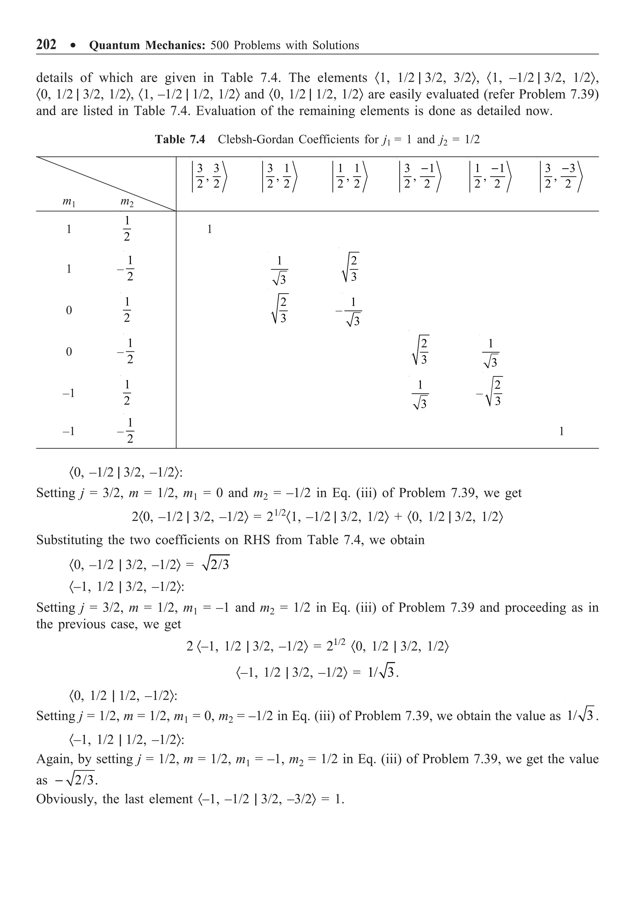
213. Angular Momentum and Spin ∑ 203
7.42 Obtain the matrix of Clebsh-Gordan coefficients for j1 = 1 and j2 = 1.
Solution. The nonvanishing Clebsh-Gordan coefficients can be evaluated with the help of
Tables 7.2 and 7.5. These coefficients are
·1, 1 | 2, 2Ò = ·–1, –1 | 2, –2Ò = 1
·1, 0 | 2, 1Ò = ·1, 0 | 1, 1Ò = ·0, 1 | 2, 1Ò = ·0, 1 | 2, –1Ò = ·1, –1 | 1, –1Ò
= ·–1, 0 | 2 – 1Ò = ·1, –1 | 1, 0Ò = 1/ 2
·0, 1 | 1, 1Ò = ·–1, 1 | 1, 0Ò = ·–1, 0 | 1, –1Ò = –1/ 2
·1, –1 | 2, 0Ò = ·–1, 1 | 2, 0Ò = 1/ 6
·1, –1 | 0, 0Ò = ·–1, 1 | 0, 0Ò = 1/ 3
·0, 0 | 2, 0Ò = 2/3; ·0, 0 | 0, 0Ò = –1/ 3 ; ·0, 0 | 1, 0Ò = 0
Table 7.5 Clebsh-Gordan Coefficients for 1 2 1 2
, 2 ,
m m j j
| Ò = | - Ò 1 2
1, 1
j j
| - - Ò and 1 2
2,
j j
| - Ò
m1 m2 jm
| Ò
1 2 1 2
, 2
j j j j
| + + - Ò 1 2 1 2
1, 2
j j j j
| + - + - Ò 1 2 1 2
2, 2
j j j j
| + - + - Ò
j1 j2 – 2
1/2
2 2
1 2
(2 1)
( )
j j
j j A
-
È ˘
Í ˙
+
Î ˚
1/2
1 2
1 2
(2 1)
( )
j j
j j B
-
È ˘
Í ˙
+
Î ˚
1/2
1 1
(2 1)
j j
AB
-
È ˘
Í ˙
Î ˚
j1 – 2 j2 – 1
1/2
1 2
1 2
4
( )
j j
j j A
È ˘
Í ˙
+
Î ˚
1 2
1/2
1 2
[( ) ]
j j
j j B
-
+
1/2
1 2
(2 1)(2 1)
j j
AB
- -
È ˘
- Í ˙
Î ˚
j1 – 2 j2
1/2
1 1
1 2
(2 1)
( )
j j
j j A
-
È ˘
Í ˙
+
Î ˚
1/2
2 1
1 2
(2 1)
( )
j j
j j B
-
È ˘
- Í ˙
+
Î ˚
1/2
2 2
(2 1)
j j
AB
-
È ˘
Í ˙
Î ˚
A = 2j1 + 2j2 – 1, B = j1 + j2 – 1
7.43 An electron is in a state described by the wave function
1
(cos sin ) ( ),
4
i
e R r
f
y q q
p
-
= +
2 2
0
( ) 1
R r r dr
•
| | =
Ú
where q and f are, respectively, the polar and azimuth angles: (i) What are the possible values of
Lz? (ii) What is the probability of obtaining each of the possible values of Lz?
Solution.
(i) From Table 5.2 we have
1/2
10
3
cos ,
4
Y q
p
Ê ˆ
= Á ˜
Ë ¯
1/2
1, 1
3
sin
8
i
Y e f
q
p
-
-
Ê ˆ
= Á ˜
Ë ¯
Hence the given wave function can be written as
10 1, 1
1
( 2 ) ( )
3
Y Y R r
y -
= +
The possible values of Lz are 0 and .

214. 204 ∑ Quantum Mechanics: 500 Problems with Solutions
(ii) 2 2 2 2
10 1, 1
1
( ) ( 2 ) sin
3
d R r Y Y r d d dr
y t q q f
-
| | = | | | + |
Ú Ú
2
10 1, 1
( 2 )
Y Y -
| + | = 10 1, 1 10 1, 1
( 2 )* ( 2 )
Y Y Y Y
- -
+ +
= 10 10 1, 1 1, 1 10 1, 1 1, 1 10
* * * *
2 2( )
Y Y Y Y Y Y Y Y
- - - -
+ + +
= 2 2
3 3
(cos sin ) cos sin ( )
4 4
i i
e e
f f
q q q q
p p
-
+ + +
=
3
(1 sin 2 cos )
4
q f
p
+
2
d
y t
| |
Ú =
2
2 2
0 0 0
1
( ) sin (1 sin 2 cos )
4
R r r dr d d
p p
q q q f f
p
•
| | +
Ú Ú Ú
=
0
1
sin 1
2
d
p
q q =
Ú
i.e., the given wave function is normalized. The probability density is then P = |y |2
. Hence, the
probability of obtaining Lz = 0 is 2
(1/ 3) 1/3.
= The probability of obtaining Lz = –1 is
2
( 2/3) 2/3.
=
7.44 An operator P describing the interaction of two spin-half particles is P = a + bs1 ◊ s2, where
a, b are constants, with s1 and s2 being the Pauli matrices of the two spins. The total spin angular
momentum S = S1 + S2 = (1/2) (s1 + s2). Show that P, S2
and Sz can be measured simultaneously.
Solution. P, S2
and Sz can be measured simultaneously if
2 2
[ , ] [ , ] [ , ] 0
z z
P S P S S S
= = =
We know that [S2
, Sz] = 0. From the definition
2
2 2 2
1 1 1 2
( 2 )
4
S s s s s
= + + ◊
we have
2
2 2
1 2 1 2
2
2 1
( )
2
S
s s s s
◊ = - +
Since for each particle,
2 2 2 2
3
x y z I
s s s s
= + + =
where I is the unit matrix, we have
2 2
1 2
1 1
( ) (3 3 ) 3
2 2
I I I
s s
+ = + =
Hence,
s1 ◊ s1 =
2
2
2
3
S
I
-

215. Angular Momentum and Spin ∑ 205
[S2
, P] =
2
2 2 2
1 2 2
2
[ , ] [ , ] , 3
S
S a b S b S I
È ˘
+ ◊ = -
Í ˙
Í ˙
Î ˚
s s
=
2
2 2
2
2
, [ , 3 ] 0
S
b S b S I
È ˘
- =
Í ˙
Í ˙
Î ˚
[Sz, P] = [Sz, a] +
2
2
2
, 3
z
S
b S I
È ˘
-
Í ˙
Í ˙
Î ˚
= 0
Since S2
and Sz commute with P, all the three can be measured simultaneously.
7.45 Obtain the Hamiltonian operator for a free electron having magnetic moment m in an external
magnetic field Bz in the z-direction in the electron’s reference frame. If another constant magnetic
field By is applied in the y-direction, obtain the time rate of change of m in the Heisenberg picture.
Solution. The magnetic moment of the electron is given by
2 B
e e
m m
m
= - = - = -
m s s
S
where S = 1/2 s and mB is the Bohr magneton. The Hamiltonian
B
z z z z
H B B
m m s
¢ = - ◊ = - =
m B
With the total magnetic field applied ˆ ˆ,
y z
B B y B z
= + the total Hamiltonian
H = mB (szBz + syBy)
From Eq. (3.30),
d
dt
m
= B B
1 1
[ , ] [ , ( )]
z z y y
H B B
i i
m m m s s
= - +
s
=
2
B ˆ ˆ ˆ
[ , ]
x y z z z y y
x y z B B
i
m
s s s s s
- + + +
=
2
B ˆ ˆ ˆ
[ , ] [ , ] [ , ]
x z z x y y y z z
B x B x B y
i
m
s s s s s s
- + +
ˆ ˆ ˆ
[ , ] [ , ] [ , ]
y y y z z z z y y
B y B z B z
s s s s s s
+ + +
Using the commutation relations among sx, sy, sz, we get
d
dt
m
= 2
B ˆ ˆ ˆ ˆ
[ 2 2 2 2 ]
y z z y x z x y
i
i B x i B x i B y i B z
m s s s s
- + + -
= 2
B
2
ˆ ˆ ˆ
[( ) ]
y z z y x z x y
B B x B y B z
m s s s s
- - +
= 2 2
B B
2 2
[ ] [ ]
m m
¥ = - ¥
s s
B B
= [ ]
e
m
¥ m
B
which is the time rate of change of the magnetic moment.

216. 206 ∑ Quantum Mechanics: 500 Problems with Solutions
7.46 Obtain the energy levels of a symmetric top molecule with principal moments of inertia
I1 = I2 = I π I3.
Solution. Let (x, y, z) be the coordinates of a body-fixed coordinate system. The Hamiltonian
H =
2 2
2
2 2 2
1 2 3 3
1 1 1
( )
2 2 2
y z
x
x y z
L L
L
L L L
I I I I I
Ê ˆ
+ + = + +
Á ˜
Ë ¯
= 2 2
3
1 1 1 1
2 2 z
L L
I I I
Ê ˆ
+ -
Á ˜
Ë ¯
|lmÒ are the simultaneous eigenkets of L2
and Lz. The Schrödinger equation is
2 2
3
1 1 1 1
2 2 z
L L lm E lm
I I I
È ˘
Ê ˆ
+ - | Ò = | Ò
Í ˙
Á ˜
Ë ¯
Î ˚
2 2
2
3
1 1
( 1)
2 2
lm
E l l m
I I I
Ê ˆ
= + + -
Á ˜
Ë ¯
which is the energy equation for symmetric top. This energy equation can be expressed in the
familiar form by writing
2
,
2
B
I
=
2
3
2
C
I
=
Elm = Bl (l + 1) + (C – B) m2
The constants B and C are rotational constants.
l = 0, 1, 2, º; m = 0, ±1, ±2, º, ±l
7.47 The kets | j, mÒ are the simultaneous eigenkets of J2
and Jz. Show that | j, mÒ are also eigenkets
of [Jx, J+] and of [Jy, J+]. Find the eigenvalues of each of these commutators.
Solution. Operating [Jx, J+] on the eigenkets | jmÒ, we obtain
[Jx, J+] | jmÒ = Jx J+ | jmÒ – J+Jx | jmÒ
=
1 1
( ) ( )
2 2
J J J jm J J J jm
+ - + + + -
+ | Ò - + | Ò
=
1 1 1 1
2 2 2 2
J J jm J J jm J J jm J J jm
+ + - + + + + -
| Ò - | Ò - | Ò - | Ò
=
1 1
2 2
J J jm J J jm
- + + -
| Ò - | Ò
From Problem 7.14,
J–J+ = J2
– Jz
2
– Jz, J+J– = J2
– Jz
2
+ Jz
Hence,
[Jx, J+] | jmÒ = 2 2 2 2
1 1
( ) ( )
2 2
z z z z
J J J jm J J J jm
- - | Ò - - + | Ò
= 2
z
J jm m jm
- | Ò = - | Ò

217. Angular Momentum and Spin ∑ 207
i.e., | jmÒ are eigenkets of [Jx, J+] with eigenvalues –m2
. Now,
[Jy, J+] | jmÒ = ( )
y y
J J J J jm
+ +
- | Ò
=
1 1
( ) ( )
2 2
J J J jm J J J jm
i i
+ - + + + -
- | Ò - - | Ò
=
1 1
2 2
J J jm J J jm
i i
- + + -
- | Ò + | Ò
= 2 2 2 2
1 1
( ) ( )
2 2
z z z z
J J J jm J J J jm
i i
- - - | Ò + - + | Ò
= 2
1 1
)
z
J jm m jm
i i
| Ò = | Ò
= 2
im jm
- | Ò
That is, | jmÒ are eigenkets of the commutator [Jy, J+] with the eigenvalue –im2
.
7.48 The state of the hydrogen atom is 2p state. Find the energy levels of the spin-orbit interaction
Hamiltonian AL ◊ S, where A is a constant.
Solution. The 2p state means s = 1/2, l = 1 and j = 1 + (1/2) = (3/2) or 1 – (1/2) = (1/2). The total
angular momentum
J = L + S (i)
J2
= L2
+ S2
+ 2L ◊ S
2 2 2
( )
2
so
A
H A J L S
= ◊ = - -
L S (ii)
The eigenvector associated with the variable J2
, Jz, L2
, S2 be | jmlsÒ. In this space,
2 2
( 1)
J jmls j j jmls
| Ò = + | Ò
(iii)
2 2
( 1)
S jmls s s jmls
| Ò = + | Ò
(iv)
2 2
( 1)
L jmls l l jmls
| Ò = + | Ò
(v)
Using Eqs. (ii)–(v), the energy eigenvalue of Hso is given by
j =
3
2
: Eso = 2 2 2
15 3
2
2 4 4
A È ˘
- -
Í ˙
Î ˚
= 2
2
A
j =
1
2
: Eso = 2 2 2
3 3
2
2 4 4
A È ˘
- -
Í ˙
Î ˚
= 2
A
-

218. 208 ∑ Quantum Mechanics: 500 Problems with Solutions
7.49 The Hamiltonian of a system of 3 nonidentical spin-half particles is
H = AS1 ◊ S2 – B(S1 + S2) ◊ S3
where A and B are constants are S1, S2 and S3 are the spin angular momentum operators. Find their
energy levels and their degeneracies.
Solution. Writing S = S1 + S2 + S3 and S12 = S1 + S2, we have
2 2 2
12 3 12 3
2
S S S
= + + ◊
S S
2 2 2
12 3 12 3
1
( )
2
S S S
◊ = - -
S S
Similarly,
2 2 2
1 2 12 1 2
1
( )
2
S S S
◊ = - -
S S
since S1 = 1/2 and S2 = 1/2, the possible values of the quantum number S12 = 0 and 1. When
S12 = 0, the possible values of S = 1/2 and 1/3. The Hamiltonian
H = AS1◊S2 – B(S1 + S2) ◊ S3
= 2 2 2 2 2 2
12 1 2 12 3
( ) ( )
2 2
A B
S S S S S S
- - + - -
In the basis | SMsS12S3Ò,
H | SMsS12S3Ò = 2 2 2 2 2 2
12 1 2 12 3 12 3 12 3
( ) ( )
2 2
s s
A B
S S S SM S S S S S SM S S
- - | Ò + - - | Ò
The energy is then,
E = 2
12 12 1 1 2 2
[ ( 1) ( 1) ( 1)]
2
A
S S S S S S
+ - + - +
2
12 12 3 3
[ ( 1) ( 1) ( 1)]
2
B
S S S S S S
+ + - + - +
since S1 = S2 = S3 = 1/2. Now,
12
2 2
, 12 12 12 12
3 3
( 1) ( 1) ( 1)
2 2 2 4
S S
A B
E S S S S S S
È ˘ È ˘
= + - + + - + -
Í ˙ Í ˙
Î ˚ Î ˚
As S = 1/2 when S12 = 0,
2
0,1/2
3
4
E = -
which is 2S + 1 = 2-fold degenerate. As S = 1/2 and 3/2, when S12 = 1,
E1,1/2 = 2 2
3 3 3
2 2
4 2 4 4 4
A B
Ê ˆ Ê ˆ
- + - -
Á ˜ Á ˜
Ë ¯ Ë ¯
=
2 2 2
4 4
A A
B B
Ê ˆ
- = -
Á ˜
Ë ¯

219. Angular Momentum and Spin ∑ 209
which is 2S + 1 = 2-fold degenerate. We also have
E1,3/2 =
2 2
3 15 3
2 2
2 2 2 4 4
A B
Ê ˆ Ê ˆ
- + - -
Á ˜ Á ˜
Ë ¯ Ë ¯
=
2
4 2
A B
Ê ˆ
+
Á ˜
Ë ¯
which is four-fold degenerate.
7.50 Two electrons having spin angular momentum vectors S1 and S2 have an interaction of the
type
H = A(S1 ◊ S2 – 3S1z S2z), A being constant
Express it in terms of S = S1 + S2 and obtain its eigenvalues.
Solution. The sum of the angular momenta S1 and S2 is
S = S1 + S2 (i)
S2
= 2 2
1 2 1 2
2
+ +
S S S S
S1 ◊ S2 = 2 2 2
1 2
1
( )
2
S S S
- - (ii)
From Eq. (i),
Sz = S1z + S2z
2
z
S = 2 2 2
1 2 1 2 1 2
( ) 2
z z z z z z
S S S S S S
+ = + +
S1zS2z = 2 2 2
1 2
1
( )
2 z z z
S S S
- - (iii)
Hence,
2 2 2 2 2 2
1 2 1 2 1 2 1 2
1 3
3 ( ) ( )
2 2
z z z z z
S S S S S S S S
◊ - = - - - - -
S S (iv)
In the simultaneous eigenkets | SMÒ of S2
and Sz,
1 2 1 2
( 3 )
z z
A S S SM
◊ - | Ò
S S
= 2 2 2 2 2 2
1 2 1 2
3
( ) ( )
2 2 z z z
A A
S S S SM S S S SM
- - | Ò - - - | Ò
=
2 2 2
1 3 1 3 3 1 1
( 1)
2 2 2 2 2 2 4 4
A A
S S SM M SM
È ˘ Ê ˆ
+ - ¥ - ¥ | Ò - - - | Ò
Á ˜
Í ˙ Ë ¯
Î ˚
= 2 2
[ ( 1) 3 ]
2
A
S S M SM
+ - | Ò
(v)
Since S = S1 + S2, the quantum number S can have the values
1 1
1
2 2
+ = or
1 1
0.
2 2
- = When
S = 0, M = 0 and when S = 1, M = 1, 0, –1. The eigenkets and the corresponding eigenvalues, see
Eq. (v), are as follows:

220. 210 ∑ Quantum Mechanics: 500 Problems with Solutions
| SMÒ Eigenvalues
| 0 0Ò 0
| 1 1Ò 2
1
2
A
-
| 1 0Ò 1 A2
| 1, –1Ò 2
1
2
A
-
7.51 The wave function y = c1yn1l1m1
+ c2yn2l2m2
is a combination of the normalized stationary state
wave functions ynlm. For y to be normalized, show that c1 and c2 must satisfy | c1|2
+ | c2|2
= 1.
Calculate the expectation values of L2
and Lz.
Solution. Let us evaluate the value of
·y |y Ò = 1 1 1 2 2 2 1 1 1 2 2 2
1 2 1 2
( ) ( )
n l m n l m n l m n l m
c c c c
y y y y
· + | + Ò
= 1 1 1 1 1 1 2 2 2 2 2 2
2 2
1 2
n l m n l m n l m n l m
c c
y y y y
| | · | Ò + | | · | Ò
= | c1|2
+ | c2|2
For y to be normalized, it is necessary that
·y |y Ò = | c1|2
+ | c2|2
= 1
The expectation value of L2
is
·y | L2
|y Ò = 1 1 1 2 2 2 1 1 1 2 2 2
2
1 2 1 2
( ) ( )
n l m n l m n l m n l m
c c L c c
y y y y
· + | | + Ò
= 1 1 1 1 1 1 2 2 2 2 2 2
2 2 2 2
1 2
n l m n l m n l m n l m
c L c L
y y y y
| | · | | Ò + | | · | | Ò
= 2 2 2 2
1 1 1 2 2 2
( 1) ( 1)
c l l c l l
| | + + | | +
The expectation value of Lz is
·y | Lz |y Ò = 1 1 1 2 2 2 1 1 1 2 2 2
1 2 1 2
( ) ( )
n l m n l m z n l m n l m
c c L c c
y y y y
· + | | + Ò
= 1 1 1 1 1 1 2 2 2 2 2 2
2 2
1 2
n l m z n l m n l m z n l m
c L c L
y y y y
| | · | | Ò + | | · | | Ò
= 2 2
1 1 2 2
c m + c m
| | | |
7.52 Verify that y = A sin q exp (if), where A is a constant, is an eigenfunction of L2
and Lz. Find
the eigenvalues.
Solution. The operators for L2
and Lz are
L2
=
2
2
2 2
1 1
sin
sin sin
q
q q q q f
È ˘
∂ ∂ ∂
Ê ˆ
- +
Í ˙
Á ˜
∂ ∂
Ë ¯ ∂
Í ˙
Î ˚
Lz = i
f
∂
-
∂

221. Angular Momentum and Spin ∑ 211
L2
y =
2
2
2 2
1 1
sin sin
sin sin
i
A e f
q q
q q q q f
È ˘
∂ ∂ ∂
Ê ˆ
- +
Í ˙
Á ˜
∂ ∂
Ë ¯ ∂
Í ˙
Î ˚
= ( )
2
2
1 1
sin cos sin
sin sin
i
A e f
q q q
q q q
È ˘
∂
- -
Í ˙
∂
Í ˙
Î ˚
=
2
2 cos 1
sin
sin sin
i
A e f
q
q
q q
È ˘
- - + -
Í ˙
Í ˙
Î ˚
= 2 2
1
sin (cos 1)
sin
i
A e f
q q
q
È ˘
- - + -
Í ˙
Î ˚
=
2 2
1
sin ( sin )
sin
i
A e f
q q
q
È ˘
- - + -
Í ˙
Î ˚
= 2 2
2 sin 2
i
A e f
q y
=
That is, y is an eigenfunction of L2
with the eigenvalue 22
, and hence
( sin ) sin
i i
z
L i A e A e
f f
y q q y
f
∂
= - = =
∂
The function y is an eigenfunction of Lz also with an eigenvalue .
7.53 State Pauli’s spin matrices and their eigenvectors. For Pauli’s spin matrices, prove the
following relations:
(i)
2 2 2
1
x y z
s s s
= = = .
(ii) ; ; .
x y z y z x z x y
i i i
s s s s s s s s s
= = =
(iii) 0.
x y y x y z z y z x x z
s s s s s s s s s s s s
+ = + = + =
Solution. The Pauli spin matrix s is defined by
1
2
=
S s
sx =
0 1
1 0
Ê ˆ
Á ˜
Ë ¯
, sy =
0
0
i
i
-
Ê ˆ
Á ˜
Ë ¯
, sz =
1 0
0 1
Ê ˆ
Á ˜
-
Ë ¯
sx, sy, sz are the Pauli spin matrices. From the definition it is evident that their eigenvalues are ±1.
Their eigenvectors are (refer Problem 7.21).
Matrix sx: eigenvector for +1 eigenvalue
1
1
1
2
Ê ˆ
Á ˜
Ë ¯
eigenvector for –1 eigenvalue
1
1
1
2
Ê ˆ
Á ˜
-
Ë ¯

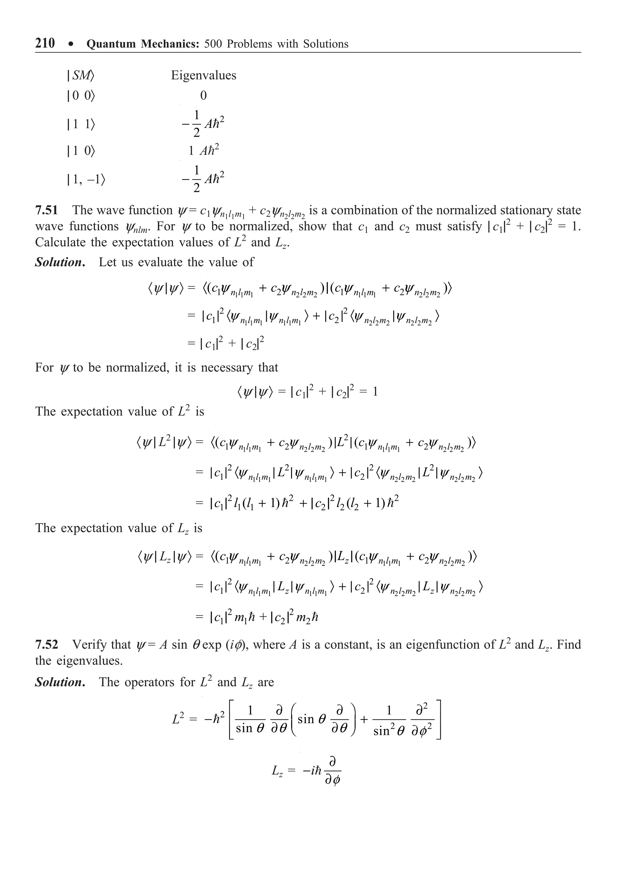
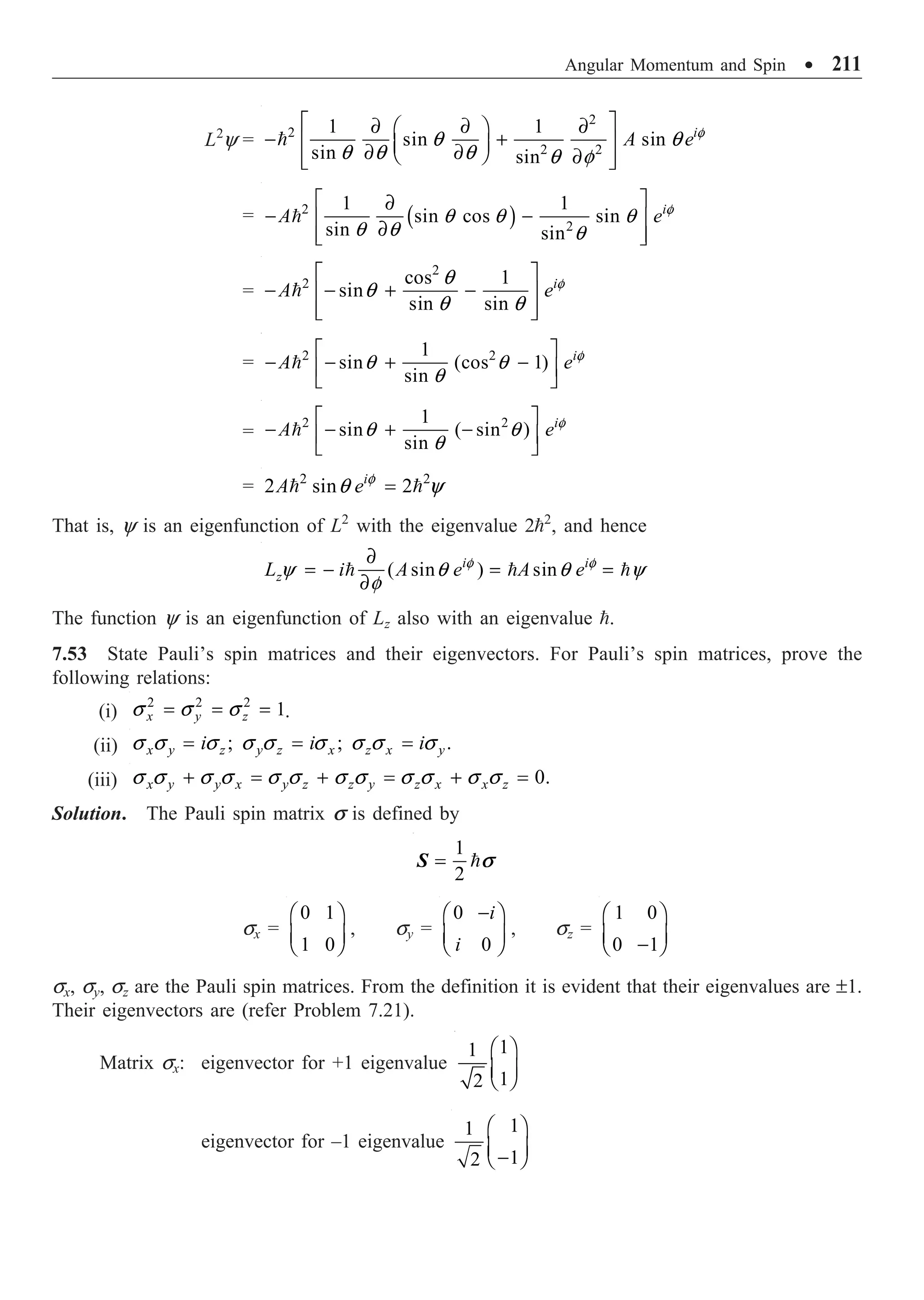
222. 212 ∑ Quantum Mechanics: 500 Problems with Solutions
Matrix sy: eigenvector for +1 eigenvalue
1
1
2 i
Ê ˆ
Á ˜
Ë ¯
eigenvector for –1 eigenvalue
1
1
2 i
Ê ˆ
Á ˜
-
Ë ¯
Matrix sz: eigenvector for +1 eigenvalue
1
1
0
2
Ê ˆ
Á ˜
Ë ¯
eigenvector for –1 eigenvalue
0
1
1
2
Ê ˆ
Á ˜
Ë ¯
(i) 2
0 1 0 1 1 0
1 0 1 0 0 1
x I
s
Ê ˆ Ê ˆ Ê ˆ
= = =
Á ˜ Á ˜ Á ˜
Ë ¯ Ë ¯ Ë ¯
Similarly, 2 2
1.
y z
s s
= =
(ii)
0 1 0 0 1 0
1 0 0 0 0 1
x y z
i i
i i
i i
s s s
-
Ê ˆ Ê ˆ Ê ˆ Ê ˆ
= = = =
Á ˜ Á ˜ Á ˜ Á ˜
- -
Ë ¯ Ë ¯ Ë ¯ Ë ¯
The same procedure gives the other relations.
(iii) x y y x
s s s s
+ =
0 1 0 0 0 1
1 0 0 0 1 0
i i
i i
- -
Ê ˆ Ê ˆ Ê ˆ Ê ˆ
+
Á ˜ Á ˜ Á ˜ Á ˜
Ë ¯ Ë ¯ Ë ¯ Ë ¯
=
0 0
0
0 0
i i
i i
-
Ê ˆ Ê ˆ
=
Á ˜ Á ˜
-
Ë ¯ Ë ¯
The same procedure proves the other relations too.
7.54 The kets | jmÒ are the simultaneous eigenkets of J2
and Jz with eigenvalues j( j + 1)2
and m,
respectively. Show that:
(i) J+ | jmÒ and J– | jmÒ are also eigenkets of J2
with the same eigenvalue.
(ii) J+ | jmÒ is an eigenket of Jz with the eigenvalue (m + 1).
(iii) J– | jmÒ is an eigenket of Jz with the eigenvalue (m – 1).
(iv) Comment on the results.
Solution. Given
J2
| jmÒ = j( j + 1)2
| jmÒ (i)
Jz | jmÒ = m | jmÒ (ii)
(i) Operating Eq. (i) from left by J+ and using the result [J2, J+] = 0, we have
J+J2
| jmÒ = j( j + 1)2
J+ | jmÒ
J2
J+ | jmÒ = j( j + 1)2
J+ | jmÒ
Similarly,
J2
J– | jmÒ = j( j + 1)2
J– | jmÒ

223. Angular Momentum and Spin ∑ 213
(ii) Operating Eq. (ii) from left by J+, we get
J+Jz | jmÒ = m J+ | jmÒ
Since [Jz, J+] = J+, J+ Jz = Jz J+ – J+.
we have
(Jz, J+ – J+) | jmÒ = mJ+ | jmÒ
Jz J+ | jmÒ = (m + 1) J+ | jmÒ
(iii) Operating Eq. (ii) from left by J– and using the result [Jz, J–] = –J–, we get
Jz J– | jmÒ = (m – 1) J– | jmÒ
(iv) J+ | jmÒ is an eigenket of Jz with the eigenvalue (m + 1) and of J2
with the same eigenvalue
j( j + 1)2
. Since operation by J+ generates a state with the same magnitude of angular
momentum but with a z-component higher by , J+ is called a raising operator. Similarly,
J– is called a lowering operator.
7.55 The two spin – half particles are described by the Hamiltonian
H = A (S1z + S2z) + B(S1 ◊ S2)
where A and B are constants and S1 and S2 are the spin angular momenta of the two spins. Find the
energy levels of the system.
Solution. Let the total angular momentum
S = S1 + S2, Sz = S1z + S2z
2 2 2
1 2 1 2
1
( )
2
S S S
◊ = - -
S S
Let the spin quantum number associated with S1 be s1 and that with S2 be S2. Since S1 = 1/2 and
S2 = 1/2, the possible values of S are 0 and 1. When S = 0, the possible values of Ms = 0. When
S = 1, the possible values of Ms = 1, 0, –1. The Hamiltonian
H = 1 2 1 2
( ) ( )
z z
A S S B
+ + ◊
S S
2 2 2
1 2
( )
2
z
B
AS S S S
+ - -
Selecting | SMsS1S2Ò as the eigenkets, we get
2 2 2
1 2 1 2 1 2 1 2
( )
2
s z s s
B
H SM S S AS SM S S S S S SM S S
| Ò = | Ò + - - | Ò
The energy
Es,Ms
= 2 3 3
( 1)
2 4 4
s
B
AM S S
È ˘
+ + - -
Í ˙
Î ˚
E0,0 = 2
3
4
B
-
E1,1 = 2
4
B
A +

224. 214 ∑ Quantum Mechanics: 500 Problems with Solutions
E1,0 = 2
4
B
E1,–1 = 2
4
B
A
- +
E00 is a singlet whereas the other three form a triplet.

225. 215
The potential energy of most of the real systems are different from those considered, and an exact
solution is not possible. Different approximate methods have therefore been developed to obtain
approximate solutions of systems. One such method is the time-independent perturbation.
8.1 Correction of Nondegenerate Energy Levels
In the time independent perturbation approach, the Hamiltonian operator H of the system is written
as
H = H0
+ H¢ (8.1)
where H0
is the unperturbed Hamiltonian, whose nondegenerate eigenvalues En
0
, n = 1, 2, 3 º, and
eigenfunctions yn
0
are assumed to be known. The functions yn
0
, n = 1, 2, 3 º, form a complete
orthonormal basis. The time-independent operator H¢ is the perturbation. The first-order correction
to the energy and wave function of the nth state are given by
y y
¢ ¢
= · | | Ò = · | | Ò
(1) 0 0
n n n
E H n H n (8.2)
y y
¢
· | | Ò
¢
= S | Ò
-
(1) 0
0 0
n m
m
n m
m H n
E E
(8.3)
where the prime on the sum means that the state m = n should be excluded. The second order
correction to the energy
¢
|· | | Ò |
¢
= S
-
2
(2)
0 0
n
m
n m
m H n
E
E E
(8.4)
8.2 Correction to Degenerate Energy Levels
When a degeneracy exists, a linear combination of the degenerate wave functions can be taken as
Time-Independent
Perturbation
CHAPTER 8

226. 216 ∑ Quantum Mechanics: 500 Problems with Solutions
the unperturbed wave function. As an example, consider the case in which En
0
is two-fold degenerate.
Let yn
0
and yl
0
be eigenfunctions corresponding to the eigenvalues En
0
= El
0
and let the linear
combination be
f = Cnyn
0
+ Clyl
0
(8.5)
where Cn and Cl constants. The first order correction to the energies are the solutions of the
determinant
(1)
(1)
0
nn n nl
nl ll n
H E H
H H E
¢ ¢
-
=
¢ ¢ -
(8.6)
The corrected energies are
+
= +
0 (1)
n n n
E E E , -
= +
0 (1)
l n n
E E E

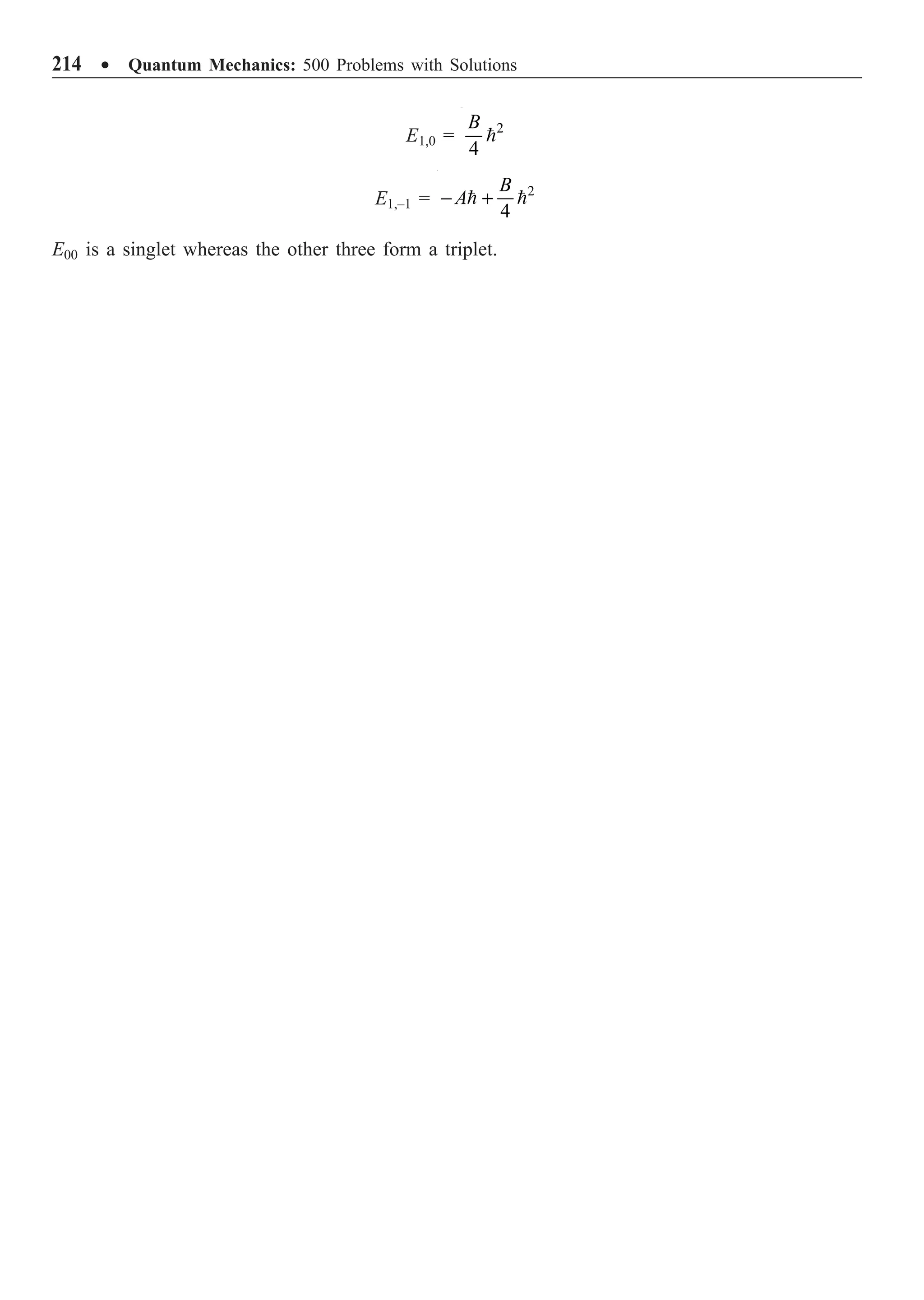
227. Time-Independent Perturbation ∑ 217
PROBLEMS
8.1 Calculate the first order correction to the ground state energy of an anharmonic oscillator of
mass m and angular frequency w subjected to a potential V(x) = 1/2 mw2
x2
+ bx4
, where b is a
parameter independent of x. The ground state wave function is
1/4 2
0
0 exp
2
m m x
w w
y
p
Ê ˆ
Ê ˆ
= -
Á ˜ Á ˜
Ë ¯ Ë ¯
Solution. The first order correction to the ground state energy
1/2 2
(1) 0 0 4
0 0
0 exp
m m x
E H b x dx
w w
y y
p
•
-•
Ê ˆ
Ê ˆ
¢
= · | | Ò = -
Á ˜ Á ˜
Ë ¯ Ë ¯
Ú
Using the result given in the Appendix, we get
1/2 5/2 2
(1)
0 2 2
3 3
2
8 4
m b
E b
m m
w p
p w w
Ê ˆ Ê ˆ
= ◊ =
Á ˜ Á ˜
Ë ¯ Ë ¯
8.2 A simple harmonic oscillator of mass m0 and angular frequency w is perturbed by an additional
potential bx3
. Evaluate the second order correction to the ground state energy of the oscillator.
Solution. The second order correction to the ground state energy is given by
2
(2)
0 0 0
0
0
,
m
m
H m
E
E E
¢
|· | | Ò|
¢
= S
-
H¢ = bx3
In terms of a†
and a,
1/2
†
0
( )
2
x a a
m w
Ê ˆ
= +
Á ˜
Ë ¯
·0 | x3
| mÒ =
3/2
0
2m w
È ˘
Í ˙
Î ˚
·0 | (a + a†
)(a + a†
)(a + a†
) | mÒ, m = 1, 2, 3, …
=
3/2
0
2m w
Ê ˆ
Á ˜
Ë ¯
[·0 | aaa | 3Ò + ·0 | aaa†
+ aa†
a |1Ò]
The other contributions vanish. For the nonvanishing contributions, we have
·0 | aaa | 3Ò = 6 , ·0 | aaa†
+ aa†
a | 1Ò = 2 + 1 = 3
3 2 2
(2) 2
0 3 4
0 0
6 9 11
2 3 8
b
E b
m m
w w w w
Ê ˆ Ê ˆ
= + = -
Á ˜
Á ˜ - -
Ë ¯
Ë ¯
8.3 Work out the splitting of the 1
P Æ 1
S transition of an atom placed in a magnetic field B along
the z-axis.
Solution. For 1
P level, S = 0 and, therefore, the magnetic moment of the atom is purely orbital. The
interaction energy between magnetic moment and the field is
0
2
z Z
e
H B L B
m
m
¢ = - =

228. 218 ∑ Quantum Mechanics: 500 Problems with Solutions
m0 is the mass of electron and Lz is the z-component of the orbital angular momentum. The first order
correction to energy of the 1
P state is
E(1)
=
0 0
,
2 2
z l
e e
lm L B lm Bm
m m
Ê ˆ
=
Á ˜
Ë ¯
ml = 1, 0, –1
The 1
P level thus splits into three levels as shown in Fig. 8.1. The 1
S level has neither orbital nor
spin magnetic moment. Hence it is not affected by the field and the 1
P Æ 1
S transition splits into
three lines.
m1
1
0
–1
B π 0
B = 0
1
S
1
P
Fig. 8.1 Splitting of 1
P Æ 1
S transition of an atom in a magnetic field.
Note: (i) If the system has more than one electron, lz = (l1z + l2z + …).
(ii) Splitting of a spectral line into three components in the presence of a magnetic field is
an example of normal Zeeman effect.
8.4 The unperturbed wave functions of a particle trapped in an infinite square well of bottom a are
yn
0
= (2/a)½
sin (npx/a). If the system is perturbed by raising the floor of the well by a constant
amount V0, evaluate the first and second order corrections to the energy of the nth state.
Solution. The first order correction to the energy of the nth state is
0 0 0 0 0 0
0 0 0
n n n n n n
H V V V
y y y y y y
¢
· | | Ò = · | | Ò = · | Ò =
Hence, the corrected energy levels are lifted by the amount V0. The second order correction to the
energy is
0 0 2 2 0 0 2
(2) 0
0 0 0 0
0
m n m n
n
m m
n m n m
H V
E
E E E E
y y y y
¢
|· | | Ò| |· | Ò|
¢ ¢
= S = S =
- -
The second order correction to the energy is zero.
8.5 A particle of mass m0 and charge e oscillates along the x-axis in a one-dimensional harmonic
potential with an angular frequency w. If an electric field e is applied along the x-axis, evaluate the
first and second order corrections to the energy of the nth state.
Solution. The potential energy due to the field e = –eex.
The perturbation H¢ = –eex.
First order correction En
(1)
= –ee ·n | x | nÒ
In terms of a and a†
,
1/2
†
0
( )
2
x a a
m w
Ê ˆ
= +
Á ˜
Ë ¯

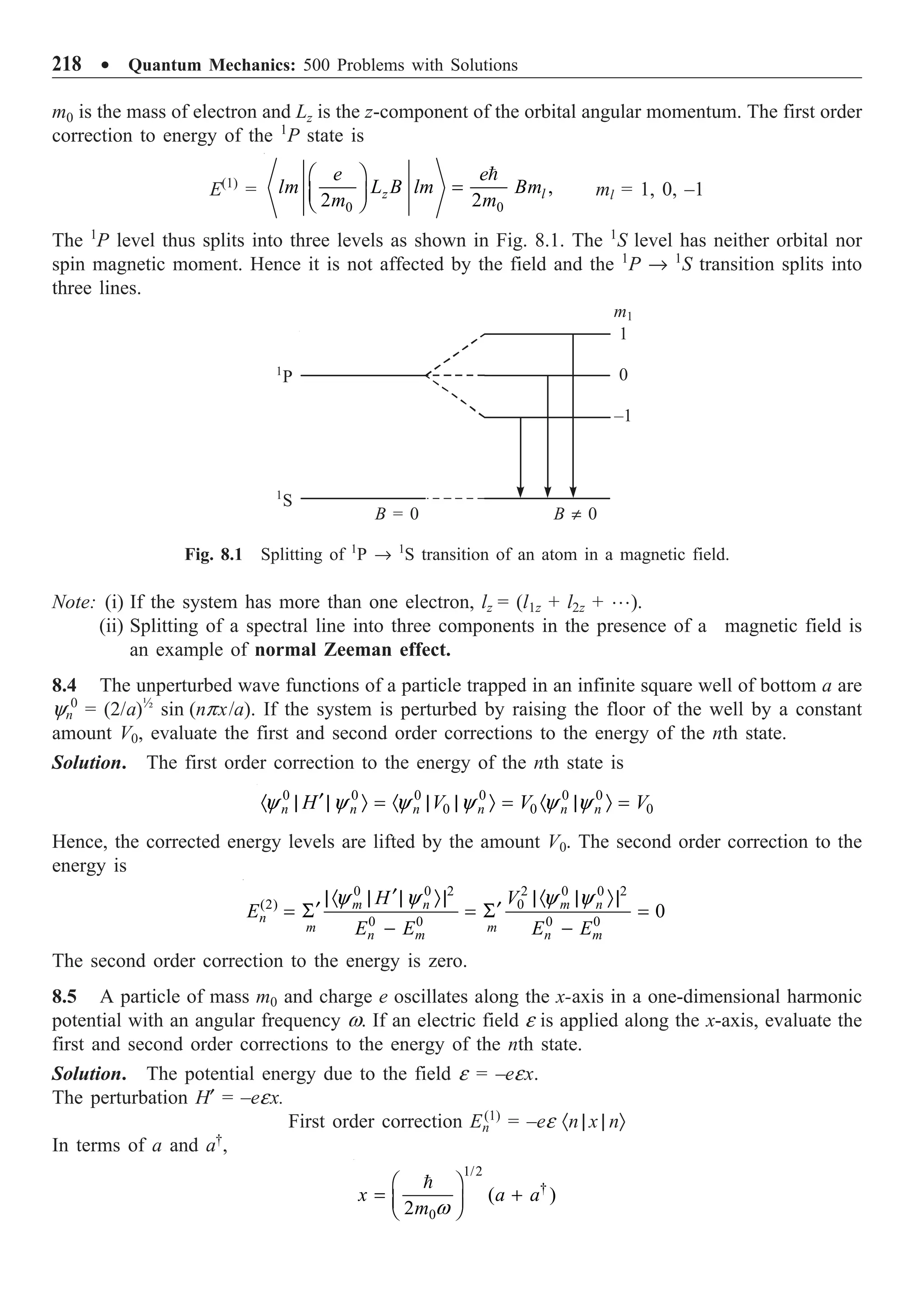
229. Time-Independent Perturbation ∑ 219
En
(1)
=
1/2
†
0
( ) 0
2
e n a a n
m
e
w
Ê ˆ
- · | + | Ò =
Á ˜
Ë ¯
En
(2)
=
2
0 0
m
n m
n H m
E E
¢
|· | | Ò|
¢
S
-
1/2
†
0
2
n H m e n a a m
m
e
w
Ê ˆ
¢
· | | Ò = - · | + | Ò
Á ˜
Ë ¯
Here, m can take all integral values except n. The nonvanishing elements correspond to m = (n +
1) and (n – 1). Hence,
2 2 2 2
(2) 2 2
2
0 0
( 1) ( )
2 2
n
n n e
E e
m m
e
e
w w w w
È ˘
+
= + = -
Í ˙
-
Í ˙
Î ˚
8.6 Evaluate the first and second order correction to the energy of the n = 1 state of an oscillator
of mass m and angular frequency w subjected to a potential
V(x) =
1
2
mw2
x2
+ bx, bx
1
2
mw2
x2
Solution. The first order correction to energy for the n = 1 state is given by
(1)
1
E =
1/2
†
1 1 1 ( ) 1
2
bx b a a
mw
Ê ˆ
· | | Ò = · | + | Ò
Á ˜
Ë ¯
=
1/2
†
[ 1 1 1 1 ] 0
2
b a a
mw
Ê ˆ
· | | Ò + · | | Ò =
Á ˜
Ë ¯
Since ( 1)
a n n n
| Ò = | - Ò and †
1 ( 1) ,
a n n n
| Ò = + | + Ò
(2)
1
E =
† 2
2 2
0 0 0 0 0 0
1 1 0 1 2
1 ( ) 1 2
2 2
k
a a k
b b
m m
E E E E E E
w w
È ˘
|· | + | Ò|
Ê ˆ Ê ˆ
¢
S = +
Í ˙
Á ˜ Á ˜
Ë ¯ Ë ¯
- - -
Í ˙
Î ˚
=
2
2
2
1 2
2 2
b
b
m m
w w w w
Ê ˆ Ê ˆ
- = -
Á ˜ Á ˜
Ë ¯ Ë ¯
8.7 Calculate the ground state energy up to first order of the anharmonic oscillator having a
potential energy V = 1/2 mw2
x2
+ ax3
; ax3
1/2 mw2
x2
, where a is independent of x.
Solution. (1) 3
0 0 0 .
E ax
= · | | Ò The integrand of this integral is an odd function of x and, therefore,
the first order correction to the ground state energy is zero.
8.8 Evaluate the first order correction to the energy of the nth state of the anharmonic oscillator
having the potential energy
V =
1
2
mw2
x2
+ bx4
, bx4
1
2
mw2
x2

230. 220 ∑ Quantum Mechanics: 500 Problems with Solutions
Solution.
(1)
n
E = n H n
¢
· | | Ò = 4
b n x n
· | | Ò
=
2
† † † †
( )( )( )( )
2
b n a a a a a a a a n
mw
Ê ˆ
· | + + + + | Ò
Á ˜
Ë ¯
The six nonvanishing matrix elements are
1. † †
( ( 1)( 2)
n aaa a n n n
· | | Ò = + +
2. † † 2
( ( 1)
n aa aa n n
· | | Ò = +
3. † †
( ( 1)
n aa a a n n n
· | | Ò = +
4. † †
( ( 1)
n a aaa n n n
· | | Ò = +
5. † † 2
(
n a aa a n n
· | | Ò =
6. † †
( ( 1)
n a a aa n n n
· | | Ò = -
Now,
(1)
n
E =
2
2 2
[( 1)( 2) ( 1) 2 ( 1) ( 1)]
2
b n n n n n n n n
mw
Ê ˆ
+ + + + + + + + -
Á ˜
Ë ¯
=
2
2
3 (2 2 1)
2
b n n
mw
Ê ˆ
+ +
Á ˜
Ë ¯
8.9 A simple harmonic oscillator of mass m and angular frequency w is perturbed by an additional
potential 1/2 bx2
. Obtain the first and second order corrections to the ground state energy.
Solution.
(1)
0
E =
2 † †
1 1
0 0 0 ( )( ) 0
2 2 2
b x b a a a a
mw
Ê ˆ
· | | Ò = · | + + | Ò
Á ˜
Ë ¯
=
†
1
0 ( 0
2 2 4
b
b aa
m m
w w
Ê ˆ
· | | Ò =
Á ˜
Ë ¯
(2)
0
E =
2
0 0
0
0
n
n
H n
E E
¢
|· | | Ò|
¢
S
-
0 H n
¢
· | | Ò =
† † † †
1
0 ,
2 2
b aa aa a a a a n
mw
Ê ˆ
· | + + + | Ò
Á ˜
Ë ¯
n π 0
= 0 ,
4
b
aa n
mw
· | | Ò
n = 2
=
2
4
b
mw
2 2 2
(2)
0 2 2 2 3
2 1
2
16 16
b b
E
m m
w
w w
= - = -
since E0 – E2 = –2w

231. Time-Independent Perturbation ∑ 221
8.10 A rotator having a moment of inertia I and an electric dipole moment m executes rotational
motion in a plane. Estimate the first and second order corrections to the energy levels when the
rotator is acted on by an electric field e in the plane of rotation.
Solution. The energy eigenvalues and eigenfunctions of a plane rotator (Problem 5.3) are
Em =
2 2
,
2
m
I
y(f) =
1
exp ( ),
2
imf
p
m = 0, ±1, ±2, …
The perturbation H¢ = –me cos f = ( )
2
i i
e e
f f
me -
- +
En
(1)
= ·n | H¢| nÒ =
2
0
cos 0
2
d
p
me
f f
p
- =
Ú
En
(2)
=
2
0 0
m
n m
n H m
E E
¢
|· | | Ò|
¢
S
-
·n | H¢ | mÒ =
2
0
( )
4
in i i im
e e e e d
p
f f f f
me
f
p
- -
- +
Ú
=
2 2
( 1 ) ( 1 )
0 0
4
i m n i m n
e d e d
p p
f f
me
f f
p
+ - - -
È ˘
- +
Í ˙
Í ˙
Î ˚
Ú Ú
The integrals are finite when m = n – 1 (first one) and m = n + 1 (second one). Therefore,
En
(2)
=
2 2 2
0 0
1 1
4 4
4 n n n n
E E E E
me p p
p - +
È ˘
Ê ˆ
- +
Í ˙
Á ˜
Ë ¯ - -
Í ˙
Î ˚
=
2 2 2 2
2 2 2
4 2 1 1
4 2 1 2 1 (4 1)
I I
n n n
me p m e
p
Ê ˆ Ê ˆ
- - =
Á ˜ Á ˜
- +
Ë ¯ Ë ¯ -
8.11 The Hamiltonian matrix of a system is
1 0
1 0 ,
0 0 2
H
e
e
Ê ˆ
Á ˜
=
Á ˜
Á ˜
Ë ¯
e 1
Find the energy eigenvalues corrected to first order in the perturbation. Also, find the eigenkets if
the unperturbed eigenkets are |f1Ò, |f2Ò and |f3Ò.
Solution. The Hamiltonian matrix can be written as
1 0 0 0 0
0 1 0 0 0
0 0 2 0 0 0
H
e
e
Ê ˆ Ê ˆ
Á ˜ Á ˜
= +
Á ˜ Á ˜
Á ˜ Á ˜
Ë ¯ Ë ¯
(i)

232. 222 ∑ Quantum Mechanics: 500 Problems with Solutions
In this form, we can identify the unperturbed part H0
and the perturbation H¢ as
0
1 0 0
0 1 0
0 0 2
H
Ê ˆ
Á ˜
=
Á ˜
Á ˜
Ë ¯
0 0
0 0
0 0 0
H
e
e
Ê ˆ
Á ˜
¢ =
Á ˜
Á ˜
Ë ¯
(ii)
The unperturbed energies are 1, 1, 2 units. The energy 1 units are two-fold degenerate. The secular
determinant corresponding to H¢ is
(1)
(1)
(1)
0
0 0
0 0
E
E
E
e
e
-
- =
-
or
2
(1) 2
0
E e
- = and E(1)
= 0
where E(1)
is the first order correction. The solution gives
E(1)
= e, –e, 0 (iii)
Hence, the state | f3Ò is not affected by the perturbation. The eigenkets corresponding to states 1 and
2 can easily be obtained. Let these states be
1 1 2 2 ,
n c c
f f f
¢ = | Ò + | Ò n = 1, 2 (iv)
The coefficients must obey the condition
–E(1)
c1 + ec2 = 0 (v)
For the eigenvalue E(1)
= e, this equation reduces to
–ec1 + ec2 = 0 or c1 = c2
Normalization gives c1 = c2 = 1/ 2 . Hence,
1 1 2
1
[ ]
2
f f f
¢ = | Ò + | Ò (vi)
With the value E(1)
= –e, Eq. (v) reduces to
ec1 + ec2 = 0 or c1 = –c2
Normalization gives c1 = –c2 = 1/ 2 . This leads to
2 1 2
1
[ ]
2
f f f
¢ = | Ò - | Ò (vii)
Thus, the corrected energies and eigenkets are
1 + e 1 2
1
[ ]
2
f f
| Ò + | Ò
1 – e 1 2
1
[ ]
2
f f
| Ò - | Ò
2 | f3Ò

233. Time-Independent Perturbation ∑ 223
8.12 A rigid rotator in a plane is acted on by a perturbation represented by
2
0
(3 cos 1)
2
V
H f
¢ = - , V0 = constant
Calculate the ground state energy up to the second order in the perturbation.
Solution. The energy eigenvalues and eigenfunctions of a plane rotator (refer Problem 5.3) are
given by
2 2
,
2
m
m
E
I
=
m = 0, ±1, ±2, º
1
( ) exp ( )
2
m im
y f f
p
=
Except the ground state, all levels are doubly degenerate. The first order correction to the ground
state energy is
(1)
0
E =
2
0
(3 cos 1)
2
V
H
y y y f y
¢
· | | Ò = -
=
2
0 0
3
cos
2 2
V V
y f y y y
-
= 0 0
0
3
4 2 4
V V
V - =
The second order energy correction
(2)
0
E =
2
0 0
0
0
m
m
H m
E E
¢
|· | | Ò|
¢
S
-
0 H m
¢
· | | Ò =
2
2
0
0
1 1
(3 cos 1)
2 2 2
im
V
e d
p
f
f f
p p
-
Ú
=
2 2
2
0 0
0 0
3
cos
4 4
im im
V V
e d e d
p p
f f
f f f
p p
-
Ú Ú
We can write cos2
f = (1 + cos 2f)/2. Also, the second integral vanishes. Hence,
2 2
0 0
0 0
3 3
0 (1 cos 2 ) cos 2
8 8
im im
V V
H m e d e d
p p
f f
f f f f
p p
¢
· | | Ò = + =
Ú Ú
since the other integral vanishes. Putting cos 2f in the exponential, we get
0 H m
¢
· | | Ò =
2
2 2
0
0
3
( )
16
i i im
V
e e e d
p
f f f
f
p
-
+
Ú
=
2 2
( 2) ( 2)
0 0
0 0
3 3
16 16
i m i m
V V
e d e d
p p
f f
f f
p p
+ -
+
Ú Ú

234. 224 ∑ Quantum Mechanics: 500 Problems with Solutions
The first integral is finite when m = –2, the second integral is finite when m = +2 and their values
are equal to 3V0/8. E±2 = 22
/I, E0 = 0. Hence,
2
0 0 0 0
0 2 0 2
2
E E E E
I
-
- = - = -
Thus,
2 2 2
(2) 0 0 0
0 2 2 2
(3 | 8) (3 | 8) 9
64
2 / 2 /
V V V I
E
I I
= + = -
- -
8.13 A plane rigid rotator in the first excited state is subjected to the interaction
2
0
(3 cos 1)
2
V
H f
¢ = -
where V0 is constant. Calculate the energies to first order in H¢.
Solution. For a plane rotator,
2 2
2
m
m
E
I
=
,
1
( ) ,
2
im
e f
y f
p
= m = 0, ±1, ±2, º
Except the m = 0 state, all states are doubly degenerate. The energy and wave function of the first
excited state are
2
1 ,
2
E
I
± =
1
( )
2
i
e f
y f
p
±
=
The first order energy corrections are given by the roots of Eq. (8.6):
(1)
11 12
1
(1)
21 22 1
H E H
H H E
¢ ¢
-
¢ ¢ -
= 0
H¢
11 =
2
2
0
22
0
1
(3 cos 1)
2 2
V
H d
p
f f
p
¢ = -
Ú
=
2 2
2
0 0 0
0 0
3 cos (3 2 )
2 2 4
V V V
d d
p p
f f f p p
p p
È ˘
- = - =
Í ˙
Í ˙
Î ˚
Ú Ú
H¢
12 =
2
2
0 0
21
0
3
1
(3 cos 1)
2 2 8
i i
V V
H e e d
p
f f
f f
p
- -
¢ = - =
Ú
The secular determinant takes the form
(1)
0 0
1
(1)
0 0
1
3
4 8
0
3
8 4
V V
E
V V
E
-
=
-
2
(1) (1)
2 0 0
1 1
5
[ ] 0
2 64
V V
E E
- - =

235. Time-Independent Perturbation ∑ 225
The roots of this equation are –(V0/8) and –(5V0/8). The corrected energies are
2
0
5
2 8
V
E
I
= +
and
2
0
2 8
V
I
-
8.14 A one-dimensional box of length a contains two particles each of mass m. The interaction
between the particles is described by a potential of the type V (x1, x2) = ld (x1 – x2), which is the
d-Dirac delta function. Calculate the ground state energy to first order in l.
Solution. The interaction between the particles can be treated as the perturbation. The Hamiltonian
without that will be the unperturbed part. Without the d-potential
1 2
1 2
0, 0 ,
( , )
, Otherwise
x x a
V x x
£ £
Ï
= Ì
•
Ô
Ó
2 2 2 2
0 1 2
2 2
1 2
( , )
2 2
d d
H V x x
m m
dx dx
= - - +
From the results of an infinitely deep potential well, the energy and wave functions are
2 2
2 2
2
( ),
2
nk
E n k
ma
p
= +
n, k = 1, 2, 3, º
1 2
1 2 1 2
2
( , ) ( ) ( ) sin sin
nk n k
n x k x
x x x x
a a a
p p
y y y
Ê ˆ Ê ˆ
= = Á ˜ Á ˜
Ë ¯ Ë ¯
For the ground state, n = k = 1, we have
2 2
0
11 2
,
E
ma
p
=
0 1 2
11 1 2
2
( , ) sin sin
x x
x x
a a a
p p
y
Ê ˆ Ê ˆ
= Á ˜ Á ˜
Ë ¯ Ë ¯
1 2
( )
H x x
ld
¢ = -
The first order correction to the ground state energy
DE = 11 11
H¢
· | | Ò
=
2
2 2
1 2
1 2 1 2
0 0
2
( ) sin sin
a a
x x
x x dx dx
a a a
p p
ld
Ê ˆ Ê ˆ
Ê ˆ
-
Á ˜ Á ˜ Á ˜
Ë ¯ Ë ¯ Ë ¯
Ú Ú
=
2
4 1
1 2
0
2 4 3 3
sin
8 2
a
x
dx a
a a a
a
p l l
l
Ê ˆ
Ê ˆ
= =
Á ˜ Á ˜
Ë ¯ Ë ¯
Ú
The corrected energy
2 2
0
11 2
3
2
E E E
a
ma
p l
¢ = + D = +
8.15 Consider the infinite square well defined by
V(x) = 0 for 0 £ x a
V(x) = • otherwise

236. 226 ∑ Quantum Mechanics: 500 Problems with Solutions
Using the first order perturbation theory, calculate the energy of the first two states of the potential
well if a portion defined by V(x) = V0x/a, where V0 is a small constant, with 0 £ x £ a being sliced
off.
Solution. From Problem 4.1, the energy eigenvalues and eigenfunctions of the the unperturbed
Hamiltonian are
2 2 2
0
2
,
2
n
n
E
ma
p
=
0 2
sin ,
n
n x
a a
p
y = n = 1, 2, 3, º
The perturbation H¢ = V0x/a which is depicted in Fig. 8.2.
a
x
0
V(x)
• •
V0
Fig. 8.2 Sliced infinite potential well.
The first order correction to the energy for the n = 1 state is
0 0
0
1 1
V x
a
y y = 2
0
0
2
sin
a
V x
x dx
a a a
p
Ú
= 0
2
0
2 2
1 cos
2
a
V x x
dx
a
a
p
Ê ˆ
-
Á ˜
Ë ¯
Ú
= 0 0
2 2
0 0
2 2 2
cos
2 2
a a
V V
x x x
dx dx
a
a a
p
-
Ú Ú
= 0 0
0
2 2
V V
+ =
The first order correction to the n = 2 state is
0 0 2
0 0 0
2 2
0
2 2
sin
2
a
V x V V
x
x dx
a a a a
p
y y = =
Ú
The corrected energies are
2 2
0
2 2
2
V
ma
p
+
and
2 2
0
2
2
2
V
ma
p
+
8.16 The energy levels of the one-electron atoms are doublets, except the s-states because of spin-
orbit interaction. The spin-orbit Hamiltonian
so 2 2
1 1
2
dV
H
r dr
m c
= ◊
L S

237. Time-Independent Perturbation ∑ 227
Treating Hso as a perturbation, evaluate the spin-orbit interaction energy. For hydrogenic atoms,
assume that the expectation value is
3
3 3
3 0
1 2
( 1)(2 1)
z
r n a l l l
=
+ +
where a0 is the Bohr radius.
Solution. For the valence electron in a hydrogen-like atom, the potential
2
0
( )
4
Ze
V r
r
pe
= - or
2
2
0
4
dV Ze
dr r
pe
= (i)
Substituting the value of dV/dr, we get
2
so 2 2 3
0
8
Ze
H
m c r
pe
◊
=
L S
(ii)
Since J = L + S,
J2
= L2
+ S2
+ 2L ◊ S or
2 2 2
2
J L S
- -
◊ =
L S (iii)
Using the basis | lsjmÒ, the expectation value of J2
– L2
– S2
is given by
·(J2
– L2
– S2
)Ò = [ j ( j + 1) – l (l + 1) – s (s + 1)] 2
(iv)
Since the first order correction to the energy constitutes the diagonal matrix elements, substituting
the values of ·1/r3
Ò and ·(J2
– L2
– S2
)Ò, we get
4 2 2
so 2 2 3 3
0 0
( 1) ( 1) ( 1)
8 ( 1)(2 1)
z e j j l l s s
E
m c a n l l l
pe
+ - + - +
=
+ +
(v)
The Bohr radius a0 and the fine structure constant a are defined as
2
0
0 2
4
a
me
pe
=
,
2
0
4
e
c
a
pe
=
(vi)
Using Eq. (vi), we get
4 2 2
so 2 2 3 3
0 0
( 1) ( 1) ( 1)
8 ( 1)(2 1)
z e j j l l s s
E
m c a n l l l
pe
+ - + - +
=
+ +
(vii)
This makes the state j = l – (1/2) to have a lower energy than that with j = l + (1/2).
8.17 The spin -orbit interaction energy
4 4 2
so 3
( 1) ( 1) ( 1)
( 1)(2 1)
2
z mc j j l l s s
E
l l l
n
a + - + - +
=
+ +
Calculate the doublet separation DEso of states with the same n and l. Apply the result to the 2p state
of hydrogen and obtain the doublet separation in units of eV.
Solution. For a given value of l, j can have the values j = l + (1/2) and j = l – (1/2). The difference
in energy between these two is the doublet separation DEso. Hence,

238. 228 ∑ Quantum Mechanics: 500 Problems with Solutions
DEso =
4 4 2
3
1 3 1 1
2 2 2 2
2 ( 1)(2 1)
z mc
l l l l
n l l l
a È ˘
Ê ˆ Ê ˆ Ê ˆ Ê ˆ
+ + - - +
Í ˙
Á ˜ Á ˜ Á ˜ Á ˜
Ë ¯ Ë ¯ Ë ¯ Ë ¯
+ + Î ˚
=
4 4 2 4 4 2
3 3
(2 1)
2 ( 1)(2 1) 2 ( 1)
z mc l z mc
n l l l n l l
a a
+
=
+ + +
For the 2p state of hydrogen, n = 2, l = 1, z = 1. So,
DEso =
31 8 1
24
4 3
(9.1 10 kg) (3 10 ms )
7.265 10 J
(137) 2 2 2
- -
-
¥ ¥
= ¥
¥ ¥ ¥
=
24
5
19
1.765 10 J
4.5 10 eV
1.6 10 J/eV
-
-
-
¥
= ¥
¥
8.18 The matrices for the unperturbed (H0
) and perturbation (H¢) Hamiltonians in the orthonormal
basis | f1Ò and | f2Ò are
H0
=
0
,
0
o
o
E
E
e
e
+
Ê ˆ
Á ˜
-
Ë ¯
H¢ =
0
0
A
A
Ê ˆ
Á ˜
Ë ¯
Determine (i) the first order correction to energy, (ii) second order correction to energy, and (iii) the
wave function corrected to first order.
Solution.
(i) The first order correction to the energy is zero since the perturbation matrix has no diagonal
element.
(ii) (2)
n
E =
2
0 0
m n m
n H m
E E
¢
|· | | Ò|
-
 ,
2 2 2
(2)
1 0 0
1 2
1 2
2 2
H A A
E
E E e e
¢
|· | | Ò| | |
= = =
-
(2)
2
E =
2 2
0 0
2 1
2 1
2
H A
E E e
¢
|· | | Ò|
=
-
-
E1 =
2
0 ,
2
A
E e
e
+ + E2 =
2
0
2
A
E e
e
- -
The wave function corrected to first order is given by
yn = 0 0
0 0
n m
m n m
m H n
E E
y y
¢
· | | Ò
+
-
Â
y1 = 1 2 1 2
0 0
1 2
2
A A
E E
f f f f
e
| Ò + = | Ò +
-
y2 = 2 1
2
A
f f
e
| Ò -

239. Time-Independent Perturbation ∑ 229
8.19 Given the matrix for H0
and H¢:
H0
=
0
0
0
,
0
E
E
Ê ˆ
Á ˜
Ë ¯
H¢ =
0
0
A
A
-
Ê ˆ
Á ˜
-
Ë ¯
In the orthonormal basis |1Ò and |2Ò, determine (i) the energy eigenvalues, and (ii) energy
eigenfunctions.
Solution. This is a case of degenerate states |1Ò and |2Ò with energy eigenvalue E0. The secular
determinant is, then,
(1)
(1)
E A
A E
- -
- -
= 0 or E(1)
= ±A
The eigenfunctions corresponding to these eigenvalues are obtained by a linear combination of |1Ò
and |2Ò. Let the combination be c1|1Ò + c2|2Ò. For +A eigenvalue, the equation (1)
11 1
1
( )
H E c
¢ -
12 2 0
H c
¢
+ = reduces to
–Ac1 – Ac2 = 0 or 1
2
1
c
c
= -
Normalization gives c1 = 1/ 2, c2 = 1/ 2. Hence, the combination is (|1Ò – |2Ò)/ 2. The other
combination is (|1Ò + |2Ò)/ 2. The energy eigenvalues and eigenfunctions are
E0 + A and (|1Ò – |2Ò)/ 2
E0 – A and (|1Ò + |2Ò)/ 2
8.20 Prove the Lande interval rule which states that in a given L-S term, the energy difference
between two adjacent J-levels is proportional to the larger of the two values of J.
Solution. For a given L-S term the total orbital angular momentum J can have the values
J = L + S, L + S – 1, º | L – S |. The spin-orbit coupling energy Eso, Problem 8.16 for a given
L-S term is
Eso = constant [J(J + 1) – L(L + 1) – S(S + 1)]
The energy difference between J – 1 and J levels is DEso given by
DEso = constant [J(J + 1) – L(L + 1) – S(S + 1) – J(J – 1) + L(L + S) + S(S + 1)]
= constant ¥ 2J
That is, the energy difference between two adjacent J-levels is proportional to the larger of the two
values of J.
8.21 An interaction of the nuclear angular momentum of an atom (I) with electronic angular
momentum (J) causes a coupling of the I and J vectors: F = I + J. The interaction Hamiltonian is
of the type Hint = constant I ◊ J. Treating this as a perturbation, evaluate the first order correction
to the energy.
Solution. Though the unperturbed Hamiltonian has degenerate eigenvalues, one can avoid working
with degenerate perturbation theory (refer Problem 8.16). The perturbing Hamiltonian
H¢ = costant I ◊ J

240. 230 ∑ Quantum Mechanics: 500 Problems with Solutions
The first order correction to energy is the diagonal matrix element of H¢ = ·H¢Ò which can be obtained
as
F2
= (I + J)2
= I2
+ J2
+ 2I ◊ J
I ◊ J =
2 2 2
2
F I J
- -
2
constant [ ( 1) ( 1) ( 1)]
2
H F F I I J J
¢
· Ò = + - + - +
Hence, the first order correction
(1)
[ ( 1) ( 1) ( 1)]
E a F F I I J J
= + - + - +
where a is a constant.
8.22 A particle in a central potential has an orbital angular momentum quantum number l = 3. If
its spin s = 1, find the energy levels and degeneracies associated with the spin-orbit interaction.
Solution. The spin-orbit interaction
so ( )
H r
x
= ◊
L S
where x (r) is a constant. The total angular momentum
J = L + S or L ◊ S = 2 2 2
1
( )
2
J L S
- -
Hence,
Hso = 2 2 2
1
( ) ( )
2
r J L S
x - -
In the | jmjlsÒ basis, the first order correction
Eso = 2 2 2
1
( ) ( )
2
j j
jm ls r J L S jm ls
x - -
= 2
1
( ) [ ( 1) ( 1) ( 1)]
2
r j j l l s s
x + - + - +
Since l = 3 and s = 1, the possible values of j are 4, 3, 2. Hence
2
2
so
2
3 ( ) , 4
( ) , 3
4 ( ) , 2
r j
E r j
r j
x
x
x
Ï =
Ô
= - =
Ì
Ô- =
Ô
Ó
The degeneracy d is given by the (2j + 1) value
9, 4
7, 3
5, 2
j
d j
j
=
Ï
Ô
= =
Ì
Ô =
Ó

241. Time-Independent Perturbation ∑ 231
8.23 Consider the infinite square well
V(x) = 0 for –a £ x £ a
V(x) = • for | x | a
with the bottom defined by V(x) = V0x/a, where V0 constant, being sliced off. Treating the sliced-
off part as a perturbation to the regular infinite square well, evaluate the first order correction to the
energy of the ground and first excited states.
Solution. For the regular infinite square well, the energy and eigenfunctions are given by Eqs. (4.2)
and (4.3).
2 2
0
1 2
,
8
E
ma
p
=
0
1
1
cos
2
x
a
a
p
y =
2 2
0
2 2
,
2
E
ma
p
=
0
2
1
sin
x
a
a
p
y =
The portion sliced off is illustrated in Fig. 8.3.
0
–a a
• •
V(x)
V0
Fig. 8.3 Infinite square well with the bottom sliced off.
Perturbation 0
V x
H
a
¢ =
The first order correction to the ground state energy is
(1) 2
0
1 2
1 1 cos 0
2
a
a
V x
E H x dx
a
a
p
-
¢
= · | | Ò = =
Ú
since the integrand is odd. The first order correction to the first excited state is
(1) 0 0 2
0 0
2 2
2 2
sin 0
a
a
V x V x
E x dx
a a
a
p
y y
-
= = =
Ú
since the integrand is odd.
8.24 Draw the energy levels, including the spin-orbit interaction for n = 3 and n = 2 states of
hydrogen atom and calculate the spin-orbit doublet separation of the 2p, 3p and 3d states. The
Rydberg constant of hydrogen is 1.097 ¥ 107
m–1
.

242. 232 ∑ Quantum Mechanics: 500 Problems with Solutions
The doublet separation
4 2
3
( 1)
Z R
E
n l l
a
D =
+
For the 2p state, n = 2, l = 1, and hence
2 7 1
1
2p
(1/137) (1.097 10 m )
( ) 36.53 m
8 2
E
-
-
¥
D = =
¥
For the 3p state, n = 3, l = 1, and so
2 7 1
1
3p
(1/137) (1.097 10 m )
( ) 10.82 m
27 2
E
-
-
¥
D = =
¥
For the 3d state n = 3, l = 2 and, therefore,
2 7 1
1
3d
(1/137) (1.097 10 m )
( ) 3.61 m
27 2 3
E
-
-
¥
D = =
¥ ¥
Note: The doublet separation decreases as l increases. The 2p doublet separation is greater than the
3p doublet which will be greater than the 4p separation (if evaluated), and so on. The d-electron
doublet splitting are also similar.
8.25 A hydrogen atom in the ground state is placed in an electric field e along the z-axis. Evaluate
the first order correction to the energy.
Solution. Consider an atom situated at the origin. If r is the position vector of the electron, the
dipole moment
m = –er
The additional potential energy in the electric field e is –m ◊ e, where q is the angle between vectors
r and e. This energy can be treated as the perturbation
H¢ = er e cos q
The unperturbed Hamiltonian
2 2
0 2
0
2 4
e
H
r
m pe
= - — -
Solution. Figure 8.4 represents the energy level for n = 3 and n = 2 states of hydrogen (Z = 1),
including the spin-orbit interaction.
j j j
1/2
1/2
1/2
3p
2p
3s
2s
3/2
1/2
3/2
3d 3/2
5/2
Fig. 8.4 Energy levels for n = 3 and n = 2 states of hydrogen.

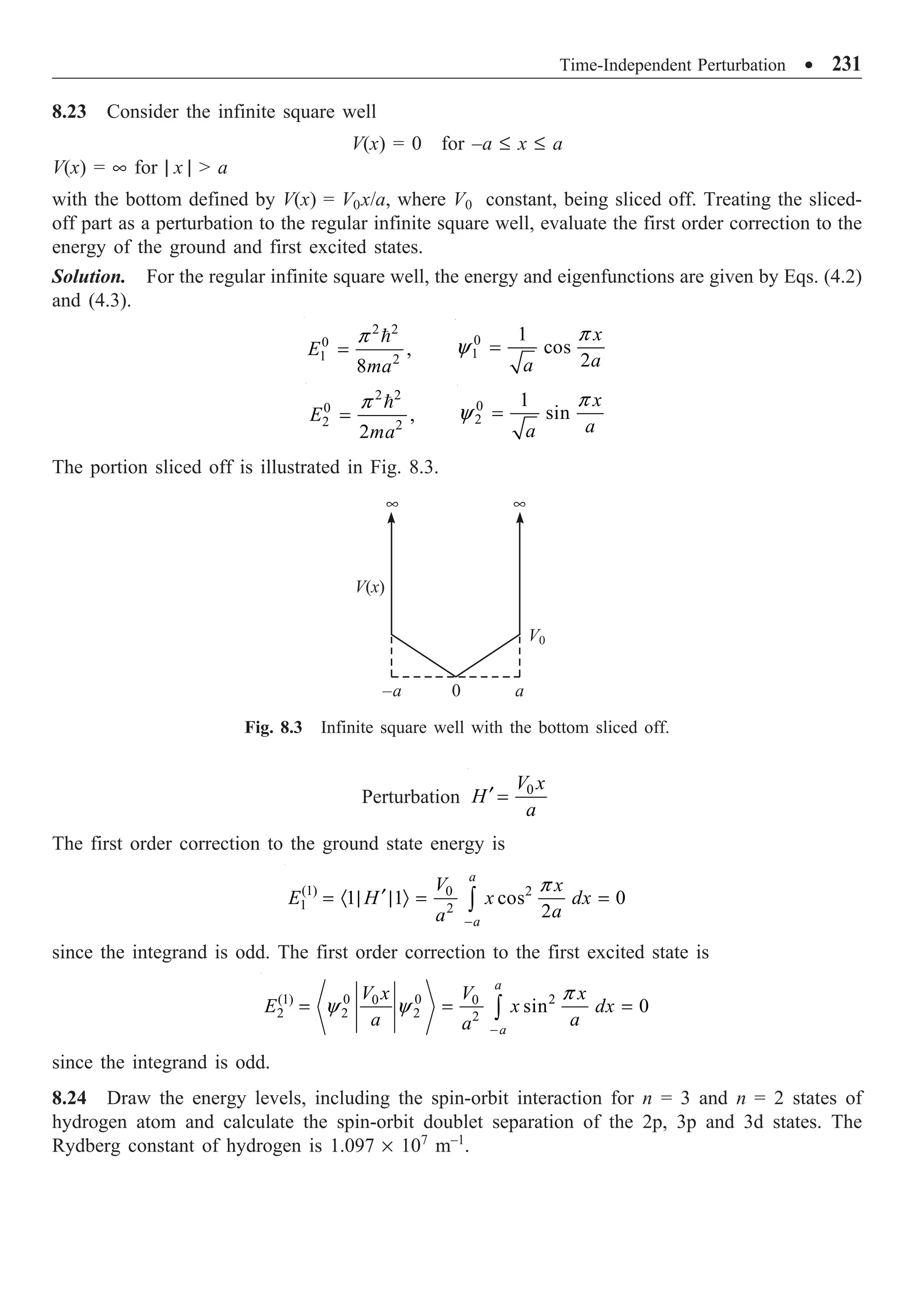
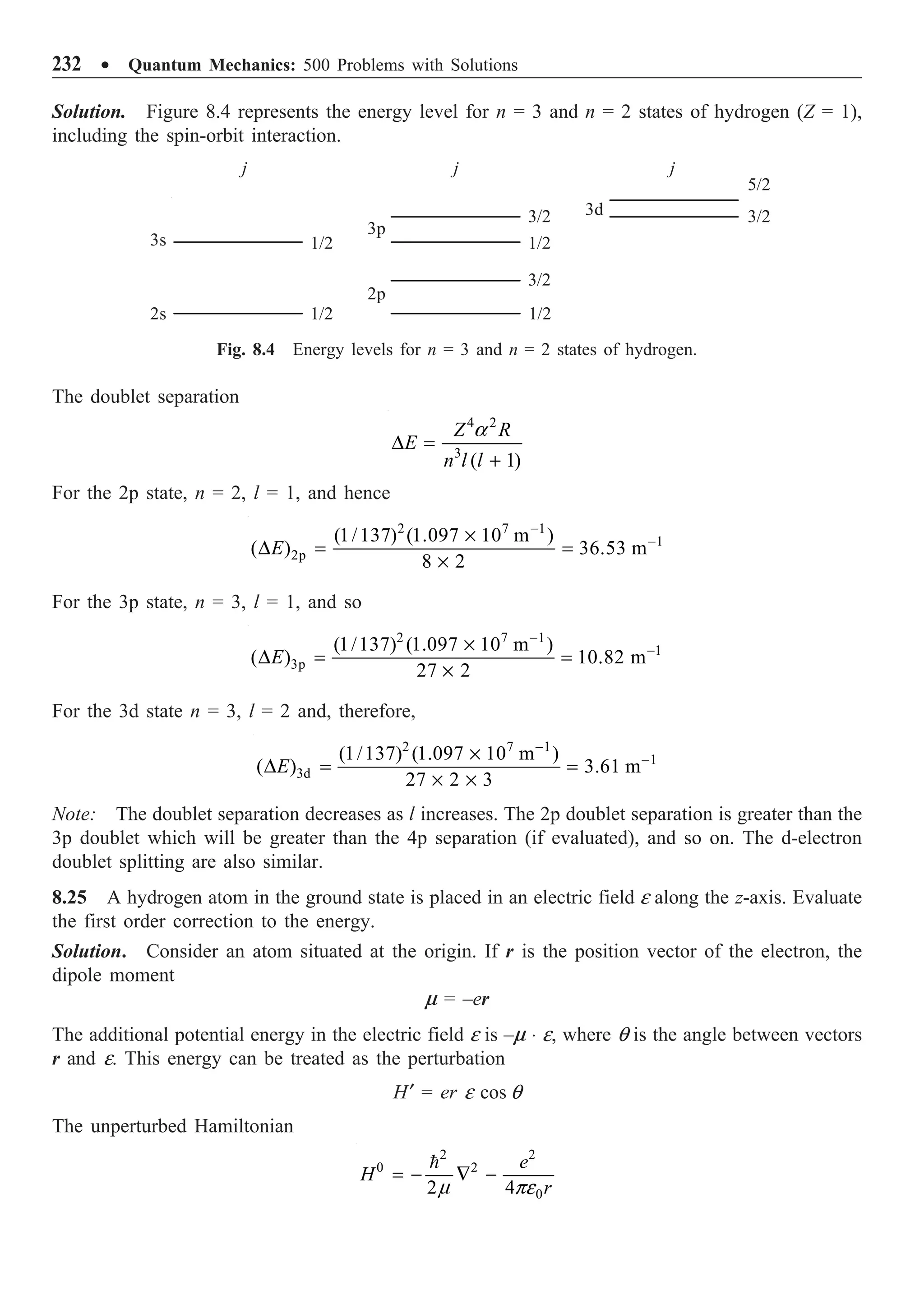
243. Time-Independent Perturbation ∑ 233
The unperturbed wave function
0
/
100 1/2 3/2
0
1 r a
e
a
y
p
-
= -
The first order correction to the energy
(1)
100 cos 100
l
E ere q
= · | | Ò
The angular part of this equation is
0
cos sin 0
d
p
q q q =
Ú
i.e., the first order correction to the energy is zero.
8.26 A particle of mass m moves in an infinite one-dimensional box of bottom a with a potential
dip as defined by
V(x) = • for x 0 and x a
V(x) = –V0 for 0
3
a
x
V(x) = 0 for
3
a
x a
Find the first order energy of the ground state.
Solution. For a particle in the infinite potential well (Fig. 8.5) defined by V(x) = 0 for 0 x a
and V(x) = • otherwise, the energy eigenvalues and eignfunctions are
2 2 2
2
2
n
n
E
ma
p
=
,
2
sin ,
n
n x
a a
p
y = n = 1, 2. 3, º
The perturbation H¢ = –V0, 0 x (a/3). Hence, the first order energy correction to the ground state
is
E(1)
=
/3
2
0
0
2
sin
a
x
V dx
a a
p
- Ú
=
/3
0
0
2 1 2
1 cos
2
a
x
V dx
a a
p
Ê ˆ
- -
Á ˜
Ë ¯
Ú
3
a
- =
/3
/3
0 0
0
0
2
[ ] sin
2
a
a
V V a x
x
a a a
p
p
È ˘
- + Í ˙
Î ˚
= 0 0
0
0.866 0.264
3 4
V V
V
p
- + ¥ = -
The energy of the ground state corrected to first order is
2 2
0
2
0.264
2
E V
ma
p
= -
V(x)
0
–V0 x
a
–a/3
Fig. 8.5 Infinite square well with
potential dip.

244. 234 ∑ Quantum Mechanics: 500 Problems with Solutions
8.27 A particle of mass m moves in a one-dimensional potential well defined by
0
2
2
0 for 2 and
( ) for 2 and
for
a
a
a x a a x
V x x a x
V a x a
-
- -
Ï
Ô
= •
Ì
Ô -
Ó
Treating V0 for –a x a as perturbation on the flat bottom box V(x) = 0 for –2a x 2a and
V(x) = • otherwise, calculate the energy of the ground state corrected up to first order.
Solution. The unperturbed energy and wave function of the ground state is
2 2
0
1 2
32
E
ma
p
=
0
1
1
cos
4
2
x
a
a
p
y =
The first order correction to the energy
E(1)
= 2
0 0 1
cos 1 cos
2 4 2 2 2
a a
a a
V V
x x
dx dx
a a a a
p p
- -
Ê ˆ
= +
Á ˜
Ë ¯
Ú Ú
= 0 0 2
( ) sin
4 4 2
a
a
a
a
V V a x
x
a a a
p
p
-
-
Ê ˆ
+ Á ˜
Ë ¯
= 0 0
0
1 1
2 2
V V
V
p p
Ê ˆ
+ = +
Á ˜
Ë ¯
The corrected ground state energy
2 2
1 0
2
1 1
2
32
E V
ma
p
p
Ê ˆ
= + +
Á ˜
Ë ¯
8.28 A particle of mass m moves in an infinite one dimensional box of bottom 2a with a potential
dip as defined by
V(x) = • for x –a and x a
V(x) = –V0 for
3
a
a x
- -
V(x) = 0 for
3
a
x a
-
Find the energy of the ground state corrected to first order.
Solution. The unperturbed part of the Hamiltonian is that due to a particle in an infinite potential
defined by V(x) for –a x a and V(x) = • otherwise. The unperturbed ground state energy and
eignfunctions are
2 2
1 2
,
8
E
ma
p
=
1
1
cos
2
x
a
a
p
y =

245. Time-Independent Perturbation ∑ 235
The perturbation H¢ = –V0, –a x –(a/3). The first order correction is
E(1)
=
/3 /3
2
0 0
cos 1 cos
2 2
a a
a a
V V
x x
dx dx
a a a a
p p
- -
- -
Ê ˆ
- = - +
Á ˜
Ë ¯
Ú Ú
=
/3
/3
0 0
( ) sin
2
a
a
a
a
V V a x
x
a a a
p
p
-
-
-
-
Ê ˆ
- - Á ˜
Ë ¯
= 0 0 0 0
sin 60 0.866
3 2 3 2
V V V V
p p
- + ∞ = - + ¥
(1)
1
E = 0.195V0
The ground state energy corrected to first order is
2 2
0
2
0.195
8
E V
ma
p
= -
8.29 A hydrogen atom in the first excited state is placed in a uniform electric field e along the
positive z-axis. Evaluate the second order correction to the energy. Draw an energy level diagram
illustrating the different states in the presence of the field. Given
y200 = 0
3/2
/2
1/2
0 0
1 1
1
2 2
r a
r
e
a a
p
-
Ê ˆ Ê ˆ
-
Á ˜ Á ˜
Ë ¯ Ë ¯
y210 = 0
5/2
/2
1/2
0
1 1
cos
2
r a
re
a
q
p
-
Ê ˆ
Á ˜
Ë ¯
1
0
!
n ax
n
n
x e dx
a
•
-
+
=
Ú
Solution. The first excited state (n = 2) is four-fold degenerate. The possible (l, m) values are (0,0),
(1,0), (1,1) and (1,–1). The four degerate states are | nlmÒ: | 200Ò, | 210Ò, | 211Ò, and | 21, –1Ò. The
additional potential energy in the field can be taken as the perturbation, i.e.,
H¢ = ere cos q (i)
The energy of the n = 2 state, E2
0
is the unperturbed energy. Out of the 12 off-diagonal elements,
in 10 we have the factor
2
( )
0
i m m
e d
p
f
f
¢-
Ú
which is equal to zero if m¢ π m. Only two off-diagonal elements will be nonvanishing; these are
200 cos 210
ere q
· | | Ò = 0
2
/
4 2
4
0
0 0 0
0
1 cos sin
2
16
r a
e r
r e dr d d
a
a
p p
e
q q q f
p
•
-
Ê ˆ
-
Á ˜
Ë ¯
Ú Ú Ú
= 0
5
/
2 4
4
0
0 0
0
2
cos sin
2
16
r a
e r
d r e dr
a
a
p
e p
q q q
p
•
-
Ê ˆ
-
Á ˜
Ë ¯
Ú Ú (ii)

246. 236 ∑ Quantum Mechanics: 500 Problems with Solutions
The integral in q is very straightforward. The integral in the variable r can be evaluated with the data
given. Then,
2
0
2
cos sin
3
d
p
q q q =
Ú (iii)
0
5
/
4 5
0
0
0
36
2
r a
r
r e dr a
a
•
-
Ê ˆ
- = -
Á ˜
Ë ¯
Ú (iv)
Substituting these integrals in Eq. (ii), we get
5
0 0
4
0
2
200 210 (36 ) 3
3
8
e
H a ea
a
e
e
¢
· | | Ò = ¥ = - (v)
Then the perturbation matrix is
0
0
( ) (200) (210) (211) (21, 1)
(200) 0 3 0 0
(210) 3 0 0 0
(211) 0 0 0 0
(21, 1) 0 0 0 0
nlm
ea
ea
e
e
Æ -
Ø
-
-
-
(vi)
and the secular determinant is
(1)
0
2
(1)
0 2
(1)
2
(1)
2
3 0 0
3 0 0
0
0 0 0
0 0 0
E ea
ea E
E
E
e
e
- -
- -
=
-
-
(vii)
The four roots of this determinant are 3ea0e, –3ea0e, 0 and 0. The states | 200Ò and | 210Ò are affected
by the electric field, whereas the states | 211Ò and | 21, –1Ò are not. Including the correction, the
energy of the states are
0
2 0
3
E ea e
- , 0
2
E and 0
2 0
3
E ea e
+
This is illustrated below (The eigenstates are also noted these).
˘
˙
˙
˙
˙
˙
˚
˘
˙
˙
˙
˙
˙
˚
Energy
e = 0 e π 0 Eigenstate
0
2 0
3
E ea e
+
0
2 0
3
E ea e
-
0
2
E
1
( 200 210 )
2
| Ò - | Ò
211 , 21, 1
| Ò | - Ò
1
( 200 210 )
2
| Ò + | Ò

247. Time-Independent Perturbation ∑ 237
Note: The electric field has affected the energy means that the atom has a permanent magnetic
moment. The states | 211Ò and | 21, –1Ò do not possess dipole moment and therefore do not have first
order interaction.
8.30 The ground state of the Hydrogen atom is split by the hyperfine interaction. Work out the
interaction energy using first order perturbation theory and indicate the level diagram.
Solution. Hyperfine interaction is one that takes place between the electronic angular momentum
and the nuclear spin angular momentum. Hydrogen atom in the ground state has no orbital angular
momentum. Hence the electronic angular momentum is only due to electron spin and the interaction
is simply between the intrinsic angular momenta of the electron (Se) and proton (Sp); both are
spin-half particles. The resultant angular momentum
I = Se + Sp
Se ◊ Sp = 2 2 2
1
( )
2 e p
I S S
- -
Since both are spin half particles, the possible values of I are 0 and 1. I = 0 corresponds to a singlet
state and I = 1 to a triplet state.
·Se ◊ SpÒ = 2
1 1 3 1 3
( 1)
2 2 2 2 2
I I
È ˘
+ - ¥ - ¥
Í ˙
Î ˚
=
2
2
3
, 0 (singlet state)
4
1
, = 1 (triplet state)
4
I
I
Ï
- =
Ô
Ô
Ì
Ô
Ô
Ó
The hyperfine interaction causes the ground state to split into two, a singlet (I = 0) and a triplet
(I = 1), see Fig. 8.6.
I = 1 (triplet)
I = 0 (singlet)
(a) (b)
Fig. 8.6 Energy level: (a) without hyperfine interaction; (b) with hyperfine interaction.
8.31 Consider an atomic electron with angular momentum quantum number l = 3, placed in a
magnetic field of 2 T along the z-direction. Into how many components does the energy level of the
atom split. Find the separation between the energy levels.
Solution. For l = 3, m can have the values 3, 2, 1, 0, –1, –2, –3. The interaction Hamiltonian
H¢ = –m ◊ B, where m is the magnetic moment of the electron which is given by
0
2
e
m
= - L
m

248. 238 ∑ Quantum Mechanics: 500 Problems with Solutions
Here, L is the orbital angular momentum of the electron and m0 is its rest mass.
0 0
2 2 z
e eB
H L
m m
¢ = ◊ =
L B
In the | lmÒ basis, the energy
0 0
2 2 B
eB e
E m Bm Bm
m m
m
= = =
where mB is the Bohr magneton which has a value of 9.27 ¥ 10–24
J/T. Since m can have seven
values, the energy level splits into seven. The energies of these seven levels are
3mBB, 2mBB, 1mBB, 0, –1mBB, –2mBB, –3mBB
The lines are equally spaced and the separation between any two is
mBB = (9.27 ¥ 10–24
J/T) ¥ 2T
= 18.54 ¥ 10–24
J
8.32 A system described by the Hamiltonian H = aL2
, where L2
is the square of the angular
momentum and a is a constant, exhibits a line spectrum where the line A represents transition from
the second excited state to the first excited state. The system is now placed in an external magnetic
field and the Hamiltonian changes to H = aL2
+ bLz, where Lz is the z-component of the angular
momentum. How many distinct lines will the original line A split into?
Solution. The Hamiltonian H = aL2
. The eigenkets are | lmÒ, l = 0, 1, 2, º, m = 0, ±1, ±2, º
The first excited state is l = 1, m = 0, ±1. The second excited state is l = 2, m = 0, ±1, ±2. In the
presence of magnetic field, H = aL2
+ bLz. The perturbation H¢ = bLz.
First order correction = ·lm | bLz | lmÒ
= bm for a given value of l
For the first excited state,
bm = b, 0, –b
For the second excited state
bm = 2b, b, 0, –b, –2b
Figure 8.7 illustrates the splitting of the two energy levels. The allowed transitions
Dl = ±1, Dm = 0, ±1
2
1
0
–1
–2
1
0
–1
m
l = 2, E = 6a2
l = 1, E = 2a2
Fig. 8.7 Transitions in the presence of magnetic field.

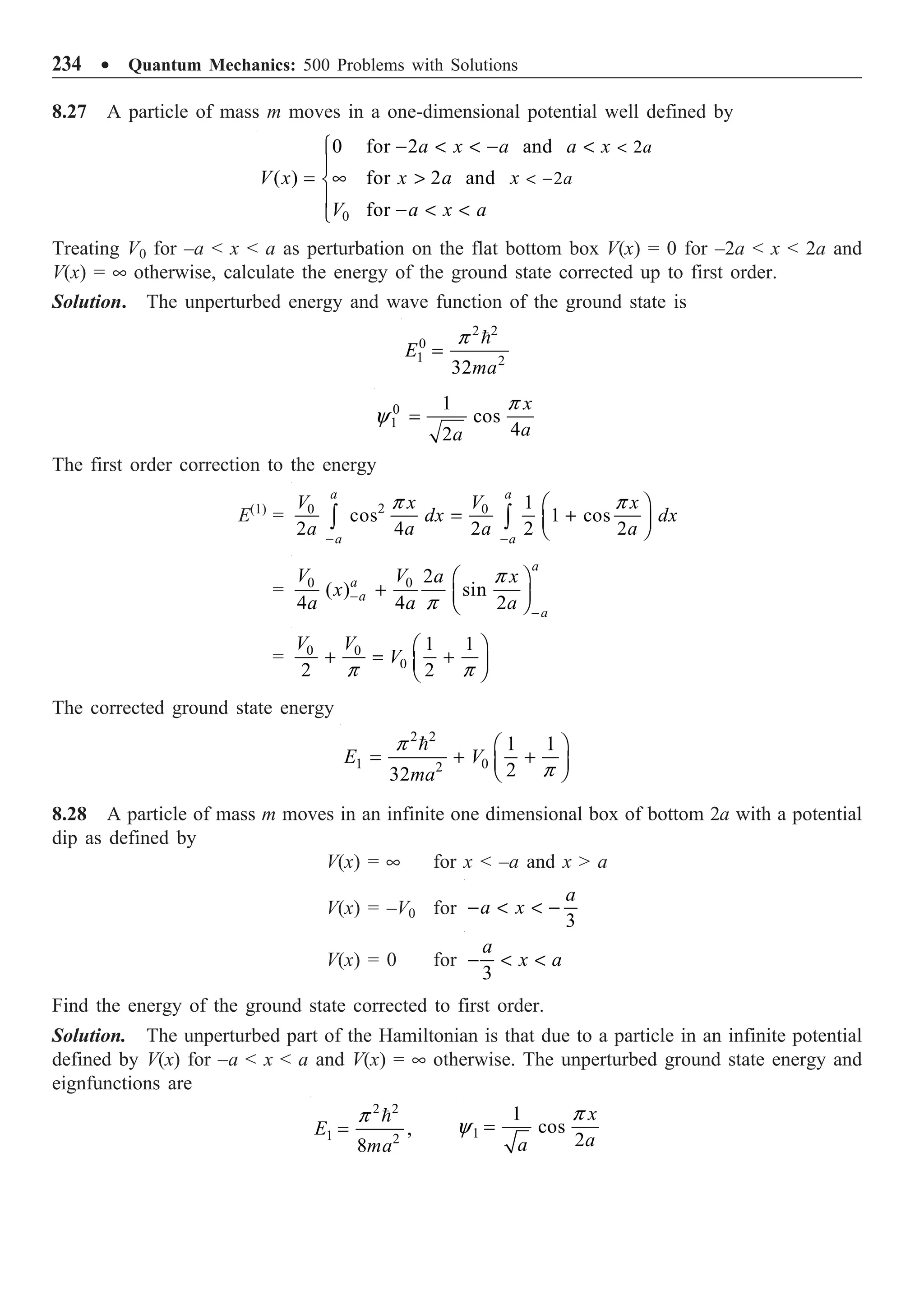
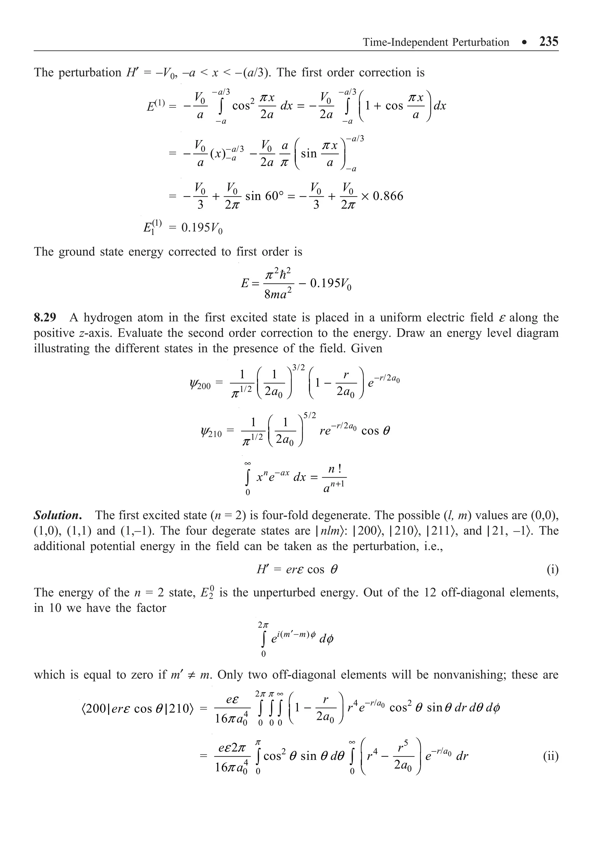
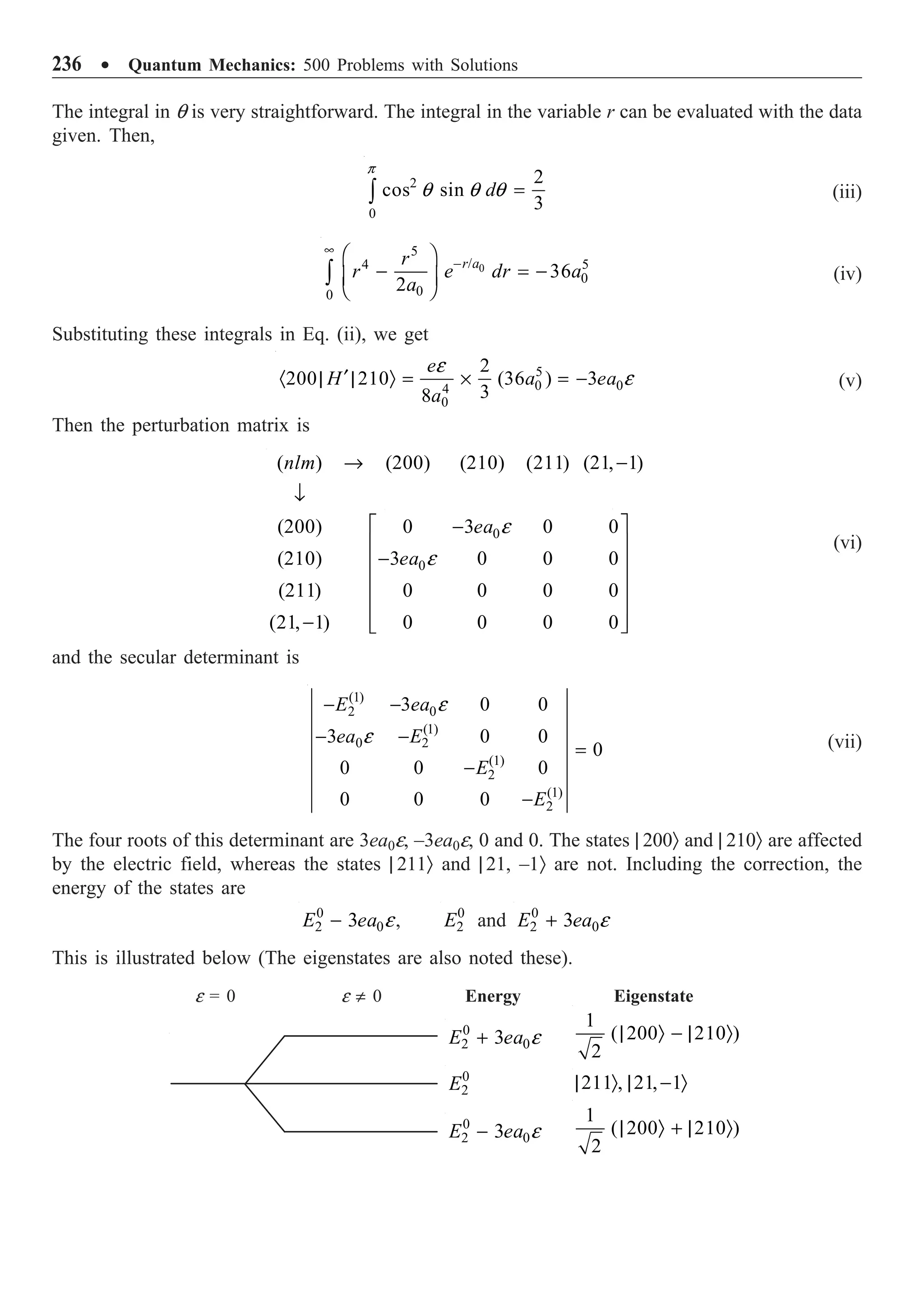
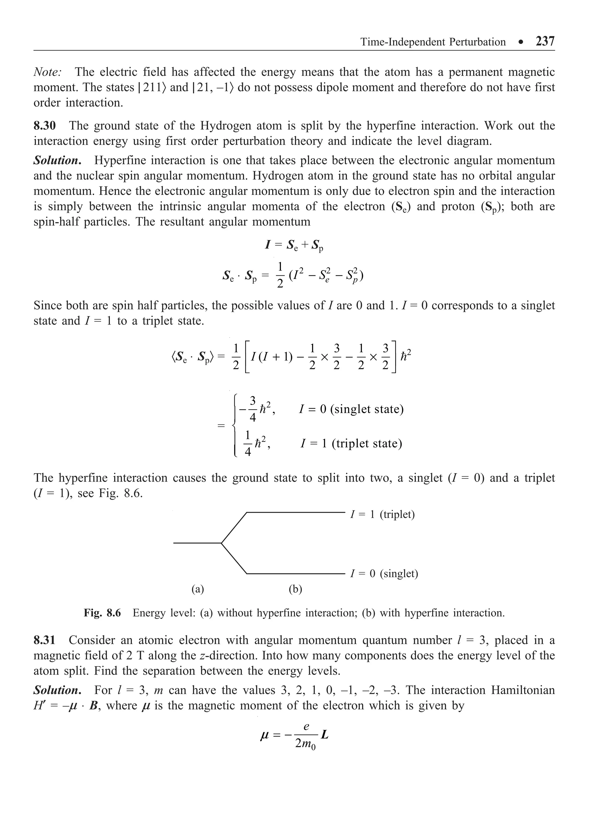
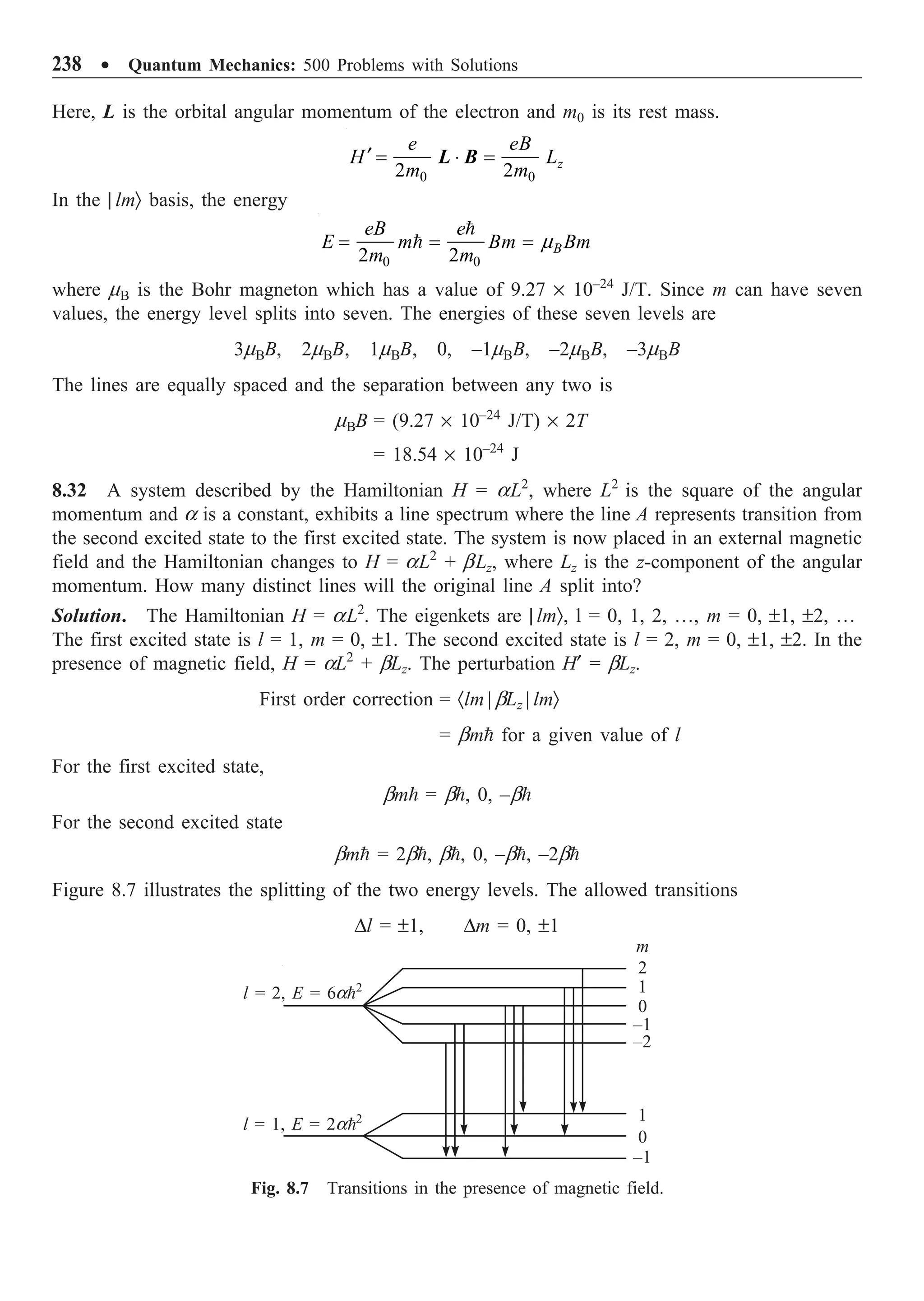
249. Time-Independent Perturbation ∑ 239
Transitions are also shown in Figure 8.7. The energies of the levels are also given, from which the
transition energies can be evaluated. The original line will split into eight lines.
8.33 The Hamiltonian of a two-electron syatem is perturbed by an interaction aS1 ◊ S2, where a
is a constant and S1 and S2 are the spin angular momenta of the electrons. Calculate the splitting
between the S = 0 and S = 1 states by first order perturbation, where S is the magnitude of the total
spin.
Solution. We have S = S1 + S2. Then,
2 2 2
1 2 1 2
2
S S S
= + + ◊
S S
2 2 2
1 2
1 2
2
S S S
- -
◊ =
S S
Since the spin of electron is 1/2 when the two electrons combine, the total spin S = 0 or 1. The state,
for which S = 0, is called a singlet state with ms = 0. The state, for which S = 1, is called a triplet
state with ms = 1, 0, –1. The first order correction to S = 0 state in the | smsÒ basis
(1)
0
E =
2 2 2
1 2
( )
2
s s
S S S
sm sm
a
- -
= 2
1 1 2 2
[ ( 1) ( 1) ( 1)]
2
s s s s s s
a
+ - + - +
= 2 2
3 3 3
0
2 4 4 4
a
a Ê ˆ
- - = -
Á ˜
Ë ¯
The first order correction to the S = 1 state is
(1)
1
E =
2
1 3 1 3
1 2
2 2 2 2 2
a È ˘
¥ - ¥ - ¥
Í ˙
Î ˚
= 2
4
a
Splitting between the two states =
2 2
3
4 4
a
a Ê ˆ
- -
Á ˜
Ë ¯
= a2
8.34 The unperturbed Hamiltonian of a system is
2
2 2
0
1
2 2
p
H m x
m
w
= +
If a small perturbation
for 0
0 for 0
x x
V
x
l
Ï
¢ = Ì
£
Ô
Ó
acts on the system, evaluate the first order correction to the ground state energy.

250. 240 ∑ Quantum Mechanics: 500 Problems with Solutions
Solution. The given H0 is the one for a simple harmonic oscillator. Hence the unperturbed ground
state energy is
1/4 2
0( ) exp
2
m m x
x
w w
y
p
Ê ˆ
Ê ˆ
= Á ˜ Á ˜
Ë ¯ Ë ¯
The first order correction to the energy is
(1)
0
E = 0 0
( ) ( )
x x x
y l y
· | | Ò
=
1/2 2
0
exp
m m x
x dx
w w
l
p
•
Ê ˆ
Ê ˆ
-
Á ˜ Á ˜
Ë ¯ Ë ¯
Ú
=
1/2
2 2
m
m m
w l
l
p w p w
Ê ˆ Ê ˆ
=
Á ˜ Á ˜
Ë ¯ Ë ¯
8.35 Consider an atomic state specified by angular momenta L, S and J = L + S placed in a
magnetic field B. Treating the interaction representing the magnetic moment of the electron in the
magnetic field as the perturbing Hamiltonian and writing L + 2S = gJ J, obtain an expression for
(i) the g factor of the Jth state are (ii) the corrected energy.
Solution. When placed in the magnetic field B, the interaction Hamiltonian
H¢ = –m ◊ B = –(mL + mS) ◊ B (i)
where mL and mS are the orbital and spin magnetic moments of the electron. We have
mL = ,
2
e
m
- L mS =
2
e
m
- S (ii)
L is the orbital angular momentum and S is the spin angular momentum. Substituting these values
of mL and mS, we get
( 2 )
e
H
m
¢ = + ◊
L S B
Given
gJJ = L + 2S
where gJ is a constant. Taking the dot product with J, we obtain
gJJ2
= J ◊ (L + 2S) = J ◊ (L + S + S)
= J ◊ (J + S) = J ◊ J + J ◊ S
= J2
+ J ◊ S
Since L = J – S,
L2
= J2
+ S2
– 2J ◊ S
J ◊ S =
2 2 2
2
J S L
+ -
gJJ2
=
2 2 2
2
2
J S L
J
+ -
+

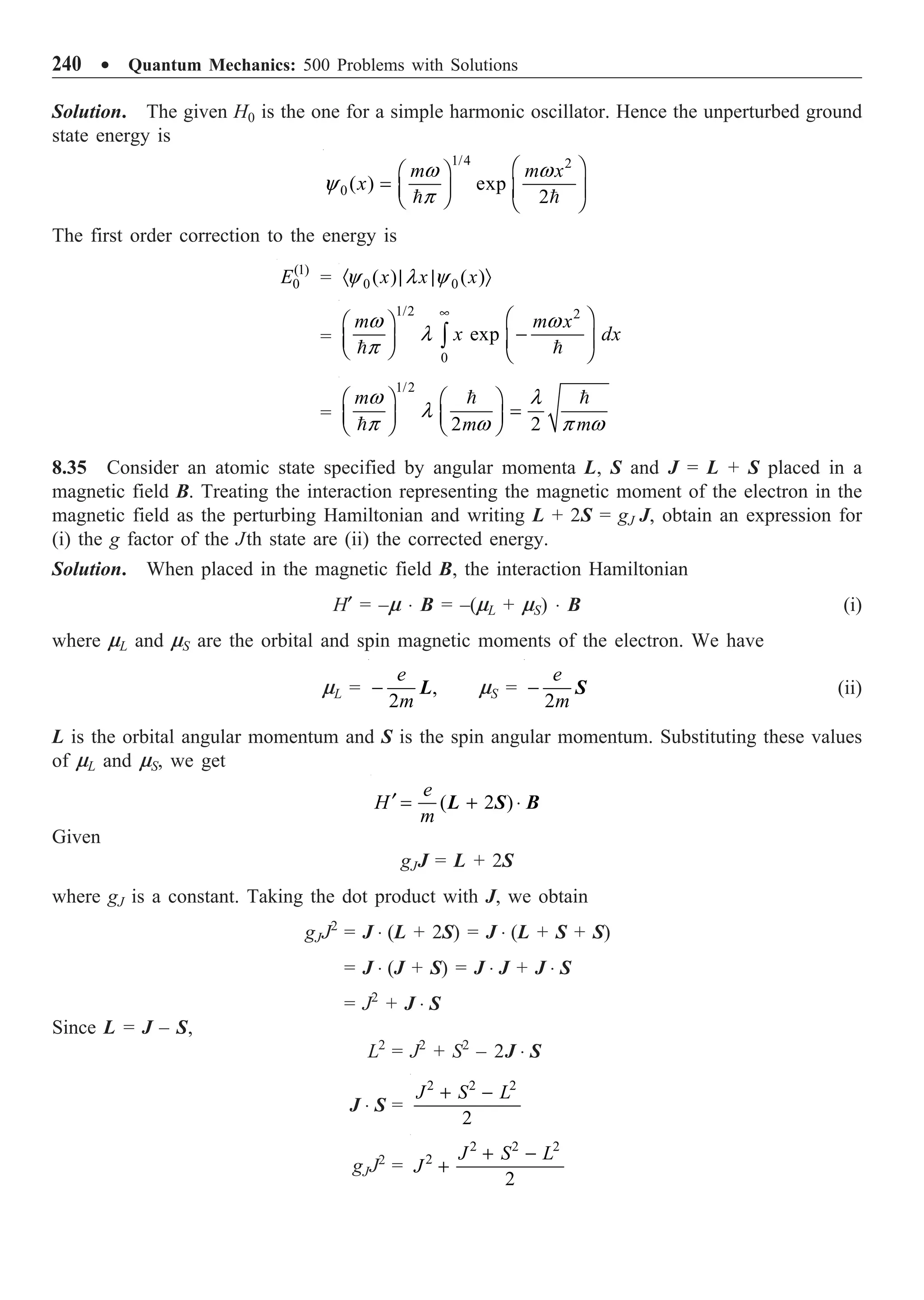
251. Time-Independent Perturbation ∑ 241
In the simultaneous eigenkets of J2
, Jz, L2
, S2
,
2 2 2 2 2
1
2
J
g J J J S L
· Ò = · Ò + · + - Ò
2 2 2
1
( 1) ( 1) [ ( 1) ( 1) ( 1)]
2
J
g J J J J J J S S L L
+ = + + + + + - +
( 1) ( 1) ( 1)
1
2 ( 1)
J
J J S S L L
g
J J
+ + + - +
= +
+
where J, L and S are the quantum numbers associated with the angular momenta J, L and S,
respectively.
(ii) The interaction Hamiltonian
H¢ = cos
2 2
e e
g gJB
m m
q
◊ =
J B
=
2 2
z
z
J
e e
gJB gBJ
m J m
=
The first order correction to the energy is the diagonal matrix element
(1)
2 2
J J J
e e
E gBM Bg M
m m
= =
The corrected energy
0
2 J J
e
E E Bg M
m
= +
Since MJ can have (2J + 1)-fold degenerate, each energy level is split into 2J + 1 equally spaced
levels.
8.36 The nuclear spin of bismuth atom is 9/2. Find the number of levels into which a 2
D5/2 term
of bismuth splits due to nuclear spin-electron angular momentum interaction. If the separation of
2
7D5/2 term from 2
6D5/2 is 70 cm–1
, what is the separation between the other adjacent levels?
Solution. 2
D5/2 term means 2S + 1 = 2, S = (1/2), L = 2 and J = (5/2). Given I = (9/2). The total
angular momentum is F = I + J. The possible values of the quantum number F are 7, 6, 5, 4, 3, 2.
Hence, the 2
D5/2 level splits into six sublevels corresponding to the F values, 7, 6, 5, 4, 3, and 2.
From Problem 8.21, we have the correction to energy as
E(1)
= a [F(F + 1) – I (I + 1) – J(J + 1)]
Hence, the energy difference DE between successive levels (F + 1) and F is given by
DE = a [(F + 1)(F + 2) – I (I + 1) – J(J + 1)] – a [F(F + 1) – I (I + 1) – J(J + 1)]
Given the separation between J = 7 and J = 6 is 70 cm–1
, i.e.,
70 cm–1
= 2a ¥ 7 or a = 5 cm–1
Hence,
2 2 1
6 5/2 5 5/2 60 cm
D D -
- =
2 2 1
5 5/2 4 5/2 50 cm
D D -
- =

252. 242 ∑ Quantum Mechanics: 500 Problems with Solutions
2 2 1
4 5/2 3 5/2 40 cm
D D -
- =
2 2 1
3 5/2 2 5/2 30 cm
D D -
- =
8.37 Discuss the splitting of atomic energy levels in a weak magnetic field and show that an energy
level of the atom splits into (2J + 1) levels. Use L-S coupling and L + 2S = gJ, where g is the Lande
g-factor, L, S and J are respectively the orbital, spin and total angular momenta of the atom.
Solution. Let m be the magnetic moment of the atom. Its orbital magnetic moment be mL and spin
magnetic moment be mS. The Hamiltonian representing the interactionof the magnetic field B with
m is
H¢ = –m ◊ B = – (mL + mS) ◊ B
Since
m = - ,
2
L
e
m
L m = - = - 2
2
S
e e
m m
S S
H¢ = ( 2 ) cos ( , )
2 2 2
e e e
g gJB
m m m
+ ◊ = ◊ =
L S B J B J B
Since (J, B) = (Jz/J),
2 2
z
z
J
e e
H gJB gBJ
m J m
¢ = =
The first order correction to energy in the common state of J2
and Jz is
E(1)
=
2
J z J
e
Jm gBJ Jm
m
=
2 2
J J
e e
gBm gBm
m m
=
= B J
gBm
m
where mB = e/2m is the Bohr magneton. As mj can have (2J + 1) values, each level splits into
2(J + 1) equally spaced levels. Hence the energy of the system
E = Enl + mBgBMJ
8.38 Discuss the splitting of atomic energy levels in a strong magnetic field. (the Paschen-Back
effect).
Solution. In a strong magnetic field, the magnetic field interaction energy is stronger than the spin-
orbit interaction energy. Hence the L–S coupling breaks. The Hamiltonian representing the
interaction of the magnetic field with m is
H¢ = –m ◊ B = – (mL + mS) ◊ B
= 2
2 2
e e
m m
◊ + ◊
L B S B
= cos ( , ) 2 cos ( , )
2 2
e e
LB B SB
m m
+
L S B

253. Time-Independent Perturbation ∑ 243
= 2
2 2
z z
L S
e e
LB SB
m L m S
+
= 2
2 2
z z
e e
BL BS
m m
+
The first order correction in the common eigenstate of L2
, Lz, S2
and Sz is
E(1)
= 2
2 2
L s
e e
Bm SBm
m m
+
= mBB(mL + 2ms)
The energy of the level becomes
( 2 )
nl B L s
E E B m m
m
= + +
8.39 A simple pendulum of length l swings in a vertical plane under the influence of gravity. In
the small angle approximation, find the energy levels of the system. Also evaluate the first order
correction to the ground state energy, taking one more term in the small angle approximation.
Solution. The first part of the problem is discussed in Problem 4.58. The energy eigenvalues and
eigenfunctions are the same as those of a linear harmonic oscillator with angular frequency
w = / ,
g l where l is the length of the pendulum. While evaluating the energy eigenvalues, we
assumed the angle q (Fig. 4 .5) to be small and retained only two terms in the expansion of cos q.
Retaining one more term, we get
cos q =
2 4
1
2 24
q q
- +
The potential is, then,
V =
2 4
(1 cos )
2 24
mgl mgl
q q
q
Ê ˆ
- = -
Á ˜
Ë ¯
=
2 4
2 24
mgl mgl
q q
-
Since q = x/l,
Perturbation
4 4
3
24 24
mgl mgx
H
l
q
¢ = - = -
The first order correction to the ground state energy is
4
(1)
0 3
0 0
24
mgx
E
l
= -
In terms of the raising and lowering operators, we have
†
( )
2
x a a
mw
= +

254. 244 ∑ Quantum Mechanics: 500 Problems with Solutions
With this value of x,
2
(1)
0 3 2
24
mg
E
m
l w
Ê ˆ Ê ˆ
= -
Á ˜ Á ˜
Ë ¯ Ë ¯
·0 | (a + a†
)(a + a†
)(a + a†
)(a + a†
) | 0 Ò
In all, there will be 16 terms on the RHS. However, only two will be nonvanishing. They are
·0 | aaa†
a†
| 0 Ò and ·0 | a a†
a a†
| 0 Ò. Consequently,
·0 | aa†
aa†
| 0 Ò = 1, ·0 | aaa†
a†
| 0 Ò = 2
Hence,
2
(1)
0 3 2
8
g
E
ml w
= -
8.40 Obtain the hyperfine splitting in the ground state of the hydrogen atom to first order in
perturbation theory, for the perturbation
H¢ = ASp ◊ Sed 3
(r), A being constant
where Sp and Se denote the spins of the proton and electron, respectively.
Solution. The hydrogen ground state wave function is
0
1/2
/
100 3
0
1 r a
e
a
y
p
-
Ê ˆ
= Á ˜
Ë ¯
The perturbation H¢ = ASp ◊ Sed 3
(r). Denoting the spin function by cs, the total wave function of the
ground state is
y = y100 cs
The first order correction to energy
(1)
0
E =
3
100 p e 100
| ( )
s s
A
y c d y c
· | Ò
i
S S r
=
3
100 100 p e
| ( ) s s
A
y d y c c
· | Ò · | | Ò
i
r S S
= p e
3
0
s s
A
a
c c
p
· | | Ò
i
S S
Writing
F = Sp + Se or Sp • Se =
2 2 2
p e
2
F S S
- -
(1)
0
E =
2 2 2
p e
3
0
2
s s
F S S
A
a
c c
p
- -
= 2
p p e e
3
0
[ ( 1) ( 1) ( 1)]
2
A
F F S S S S
a
p
+ - + - +
As Sp = (1/2) and Se = (1/2), the possible values of F are 1, 0. The separation between the two F
states is the hyperfine splitting DE. Thus,

255. Time-Independent Perturbation ∑ 245
DE = 3
0
1 3 1 3 1 3 1 3
1 2 0
2 2 2 2 2 2 2 2
2
A
a
p
È ˘
Ê ˆ Ê ˆ
¥ - ¥ - ¥ - ¥ - ¥
Í ˙
Á ˜ Á ˜
Ë ¯ Ë ¯
Î ˚
= 3
0
A
a
p
8.41 In the nonrelativistic limit, the kinetic energy of a particle moving in a potential
V(x) = 1/2mw2
is p2
/2m. Obtain the relativistic correction to the kinetic energy. Treating the
correction as a perturbation, compute the first order correction to the ground state energy.
Solution. The relativistic expression for kinetic energy is
T = 2 4 2 2 2
0 0
m c c p m c
+ -
=
1/2
2
2 2
0 0
2 2
0
1
p
m c m c
m c
Ê ˆ
+ -
Á ˜
Ë ¯
=
2 4
2 2
0 0
2 2 4 4
0 0
1
2 4
p p
m c m c
m c m c
Ê ˆ
+ - -
Á ˜
Ë ¯
=
2 4
3 2
0 0
2 8
p p
m m c
-
Perturbation H¢ =
4
3 2
0
8
p
m c
The operators a and a†
are defined by
a =
2 2
m i
x p
m
w
w
+
a†
=
2 2
m i
x p
m
w
w
-
where
p = †
2
( )
2
m
a a
i
w
-
The first order correction to the ground state energy is
(1)
0
E =
4
3 2 3 2
0 0
1
0 0
8 8
p
m c m c
Ê ˆ
- = -
Á ˜
Ë ¯
¥
2
† † † †
2
0 ( )( )( )( ) 0
4
m
a a a a a a a a
w
Ê ˆ
- - - -
Á ˜
Ë ¯
(1)
0
E =
2
† † † †
3 2
0
1 2
0 ( )( )( )( ) 0
4
8
m
a a a a a a a a
m c
w
Ê ˆ
- · | - - - - | Ò
Á ˜
Ë ¯

256. 246 ∑ Quantum Mechanics: 500 Problems with Solutions
When expanded, the expression will have 16 terms. Only two terms will be nonvanishing; these
terms are
·0 | aaa†
a†
| 0 Ò and ·0 | aa†
aa†
| 0 Ò
Since
†
| 1 | 1
a n n n
Ò = + + Ò , | | 1
a n n n
Ò = - Ò
we have
·0 | aaa†
a†
| 0 Ò = 2, ·0 | aa†
aa†
| 0 Ò = 1
Hence,
2
(1)
0 2
0
3 ( )
32
E
m c
w
= -
8.42 The Hamiltonian matrix of a system in the orthonormal basis
1
0 ,
0
Ê ˆ
Á ˜
Á ˜
Á ˜
Ë ¯
0
1 ,
0
Ê ˆ
Á ˜
Á ˜
Á ˜
Ë ¯
0
0
1
Ê ˆ
Á ˜
Á ˜
Á ˜
Ë ¯
is given by
1 2 0
2 2 3
0 3 3
H
e
e e e
e e
Ê ˆ
Á ˜
= +
Á ˜
Á ˜
+
Ë ¯
Find the energy levels corrected up to second order in the small parameter e.
Solution. The matrix H can be written as
H =
1 0 0 1 2 0
0 2 0 2 2 3
0 0 3 0 3 3
e
e e e
e e
Ê ˆ Ê ˆ
Á ˜ Á ˜
+ +
Á ˜ Á ˜
Á ˜ Á ˜
+
Ë ¯ Ë ¯
= H0
+ H¢
Identifying H0
and H¢ as the unperturbed and perturbation part, the eigenvalues of the unperturbed
Hamiltonian H0
are 1, 2 and 3. The first order correction to the energy is given by the diagonal
matrix element of H¢. Then,
H¢
11 =
0 2 0 1
(1 0 0) 2 1 3 0 0
0 3 1 0
e
Ê ˆ Ê ˆ
Á ˜ Á ˜ =
Á ˜ Á ˜
Á ˜ Á ˜
Ë ¯ Ë ¯
H¢
22 =
0 2 0 0
(0 1 0) 2 1 3 1 1
0 3 1 0
e e
Ê ˆ Ê ˆ
Á ˜ Á ˜ =
Á ˜ Á ˜
Á ˜ Á ˜
Ë ¯ Ë ¯
H¢
33 =
0 2 0 0
(0 0 1) 2 1 3 0 1
0 3 1 1
e e
Ê ˆ Ê ˆ
Á ˜ Á ˜ =
Á ˜ Á ˜
Á ˜ Á ˜
Ë ¯ Ë ¯

257. Time-Independent Perturbation ∑ 247
The first order correction to the energies are 0, 1e, 1e, respectively. The second order
correction is given by
(2)
n
E =
2
0 0
m
n m
m H n
E E
¢
|· | | Ò|
¢
S
-
12
H¢ =
0 2 0 0 2
(1 0 0) 2 1 3 1 (1 0 0) 1 2
0 3 1 0 3
e e e
Ê ˆ Ê ˆ Ê ˆ
Á ˜ Á ˜ Á ˜
= =
Á ˜ Á ˜ Á ˜
Á ˜ Á ˜ Á ˜
Ë ¯ Ë ¯ Ë ¯
13
H¢ =
0 2 0 0 0
(1 0 0) 2 1 3 0 (1 0 0) 3 0
0 3 1 1 1
e e
Ê ˆ Ê ˆ Ê ˆ
Á ˜ Á ˜ Á ˜
= =
Á ˜ Á ˜ Á ˜
Á ˜ Á ˜ Á ˜
Ë ¯ Ë ¯ Ë ¯
23
H¢ =
0 2 0 0 0
(0 1 0) 2 1 3 0 (0 1 0) 3 3
0 3 1 1 1
e e e
Ê ˆ Ê ˆ Ê ˆ
Á ˜ Á ˜ Á ˜
= =
Á ˜ Á ˜ Á ˜
Á ˜ Á ˜ Á ˜
Ë ¯ Ë ¯ Ë ¯
(2)
1
E =
2
2
2 2
31
21
4 0 4
1 2 1 3
H
H
e e
¢
¢ | |
| |
+ = - + = -
- -
(2)
2
E =
2
2
2 2 2
32
12
4 9 5
2 1 2 3
H
H
e e e
¢
¢ | |
| |
+ = - = -
- -
(2)
3
E =
2 2
2 2
13 23
0 9 9
3 1 3 2
H H
e e
¢ ¢
| | | |
+ = + =
- -
The energies of the three levels corrected to second order are
E1 = 1 + 0 – 4e2
= 1 – 4e2
E2 = 2 + e – 5e2
E3 = 3 + 1e + 9e2

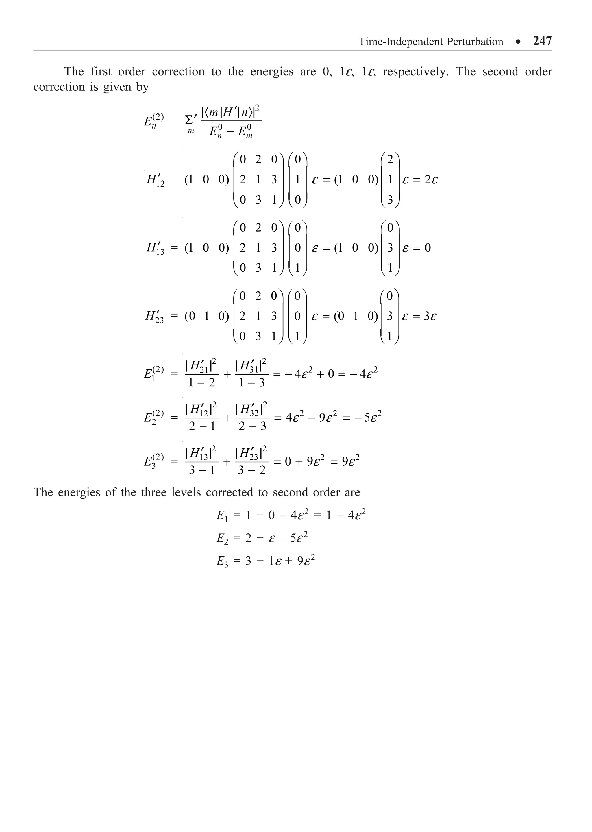
258. 248
The variation method is usually applied to obtain the ground state energy and wave functions of
quantum mechanical systems. Extension to excited states is also possible. The WKB method is based
on the expansion of the wave function of a one-dimensional system in powers of .
9.1 Variation Method
The essential idea of the method is to evaluate the expectation value ·HÒ of the Hamiltonian operator
H of the system with respect to a trial wave function f. The variational principle states that the
ground state energy
E1 £ ·HÒ = ·f | H | fÒ (9.1)
In practice, the trial function is selected in terms of one or more variable parameters and the value
of ·HÒ is evaluated. The value of ·HÒ is then minimized with respect to each of the parameters. The
resulting value is the closest estimate possible with the selected trial function. If the trial wave
function is not a normalized one, then
H
H
· | | Ò
· Ò =
· | Ò
f f
f f
(9.2)
9.2 WKB Method
The WKB method is based on the expansion of the wave function in powers of . This method is
applicable when the potential V(x) is slowly varying. When E V(x), the Schrodinger equation for
a one-dimensional system is given by
2
2
2
0,
d
k
dx
+ =
y
y 2
2
2
[ ( )]
m
k E V x
= -
(9.3)
The solution is given by
( )
exp
A
i k dx
k
= ± Ú
y (9.4)
Variation and WKB Methods
CHAPTER 9

259. Variation and WKB Methods ∑ 249
where A is a constant. The general solution will be a linear combination of the two. When E V(x),
the basic equation becomes
2
2
2
0,
d
dx
- =
y
g y 2
2
2 [ ( ) ]
m V x E
-
=
g (9.5)
Then the solution of Eq. (9.5) is
( )
exp
B
dx
= ± Ú
y g
g
(9.6)
where B is a constant.
9.3 The Connection Formulas
When E @ V(x), both the quantities k and g Æ 0. Hence, y goes to infinity. The point at which
E = V(x) is called the turning point. On one side the solution is exponential and on the other side,
it is oscillatory. The solutions for the regions E V(x) and E V(x) must be connected. The
connection formulas are as follows:
Barrier to the right of the turning point at x1:
1
1
2 1
cos exp
4
x x
x x
k dx dx
k
Ê ˆ
Ê ˆ
- ¨ -
Á ˜
Á ˜
Ë ¯ Ë ¯
Ú Ú
p
g
g
(9.7)
1
1
1 1
sin exp
4
x x
x x
k dx dx
k
Ê ˆ
Ê ˆ
- Æ - Á ˜
Á ˜
Ë ¯ Ë ¯
Ú Ú
p
g
g
Barrier to the left of the turning point at x2:
2
2
1 2
exp cos
4
x x
x x
dx k dx
k
Ê ˆ
Ê ˆ
- Æ -
Á ˜
Á ˜
Ë ¯ Ë ¯
Ú Ú
p
g
g
(9.8)
2
2
1 1
exp sin
4
x x
x x
dx k dx
k
Ê ˆ
Ê ˆ
- ¨ -
Á ˜
Á ˜
Ë ¯ Ë ¯
Ú Ú
p
g
g
The approximation breaks down if the turning points are close to the top of the barrier. Barrier
penetration: For a broad high barrier, the transmission coefficient
2
1
exp 2
x
x
T dx
Ê ˆ
= -
Á ˜
Ë ¯
Ú g (9.9)

260. 250 ∑ Quantum Mechanics: 500 Problems with Solutions
PROBLEMS
9.1 Optimize the trial function exp (–ar) and evaluate the ground state energy of the hydrogen
atom.
Solution. The trial function f = exp (–ar).
Hamiltonian of the atom H =
2 2
2
2
ke
r
- — -
m
The trial function depends only on r. Hence, —2
in the spherical polar coordinates contains only the
radial derivatives. So,
2
2 2
2 2
1 2
d d d d
r
dr dr r dr
r dr
Ê ˆ
— = = +
Á ˜
Ë ¯
From Eq. (9.2),
2 2 2
2
2
2
d d ke
H
r dr r
dr
È ˘
Í ˙
· Ò · | Ò = - + -
Í ˙
Î ˚
f f f f f f f f
m
The angular part of dt contributes a factor 4p to the integrals in the above equation. Hence,
2
2 2
2
0
4 exp ( 2 )
d
r r dr
dr
•
= - =
Ú
p
f f pa a
a
0
2 2
8 exp ( 2 )
d
r r dr
r dr
•
= - - = -
Ú
p
f f pa a
a
2 2
2
2
0
4 exp( 2 )
ke ke
e r r dr
r
•
= - =
Ú
p
f f p a
a
2
3
0
4 exp ( 2 )
r r dr
•
· | Ò = - =
Ú
p
f f p a
a
Substituting these integrals, we get
2 2
3 2
2
2
ke
H
È ˘
· Ò = - + -
Í ˙
Î ˚
p p p p
m a a
a a
2 2
2
2
H ke
· Ò = -
a
a
m
Minimizing with respect to a, we obtain
2
2
0 ke
= -
a
m
or
2
2
k e
=
m
a
With this value of a,
2 4
min min 2
2
k e
E H
= · Ò = -
m

261. Variation and WKB Methods ∑ 251
and the optimum wave function is
1/2
3
0
0
1
exp
r
a
a
Ê ˆ -
Ê ˆ
= Á ˜ Á ˜
Ë ¯
Ë ¯
f
p
where a0 is the Bohr radius.
9.2 Estimate the ground state energy of a one-dimensional harmonic oscillator of mass m and
angular frequency w using a Gaussian trial function.
Solution. The Hamiltonian of the system
2 2
2 2
2
1
2 2
d
H m x
m dx
-
= +
w
Gaussian trial function f(x) = A exp (–ax2
)
where A and a are constants. The normalization condition gives
1/2
2 2 2
1 exp ( 2 )
2
A x dx A
•
-•
Ê ˆ
= | | - = | | Á ˜
Ë ¯
Ú
p
a
a
Normalized trial function f(x) =
1/4
2
2
exp ( )
x
Ê ˆ
-
Á ˜
Ë ¯
a
a
p
2 2
2 2
2
1
2 2
d
H m x
m dx
· Ò = - + · | | Ò
f f w f f
2
2
d
dx
f f =
1/2 1/2
2 2 2 2
2 2
2 exp ( 2 ) 4 exp ( 2 )
x dx x x dx
• •
-• -•
Ê ˆ Ê ˆ
- - + -
Á ˜ Á ˜
Ë ¯ Ë ¯
Ú Ú
a a
a a a a
p p
=
1/2 1/2 1/2 1/2
2
2 2 1
2 4
2 4 2
Ê ˆ Ê ˆ Ê ˆ Ê ˆ
- + = -
Á ˜ Á ˜ Á ˜ Á ˜
Ë ¯ Ë ¯ Ë ¯ Ë ¯
a p a p
a a a
p a p a a
1/2
2 2 2
2 1
| exp ( 2 )
4
x x x dx
•
-•
Ê ˆ
· | Ò = - =
Á ˜
Ë ¯ Ú
a
f f a
p a
2 2 2
2
1 1
2 2 4 2 8
m
H m
m m
· Ò = + = +
a a w
w
a a
Minimizing with respect to a, we get
2 2
2
0
2 8
d H m
d m
· Ò
= = -
w
a a
or
m
=
w
a
With this value of a,
min
1
2
H
· Ò = w
which is the same as the value we obtained in Chapter 4. Thus, the trial wave function is the exact
eigenfunction.

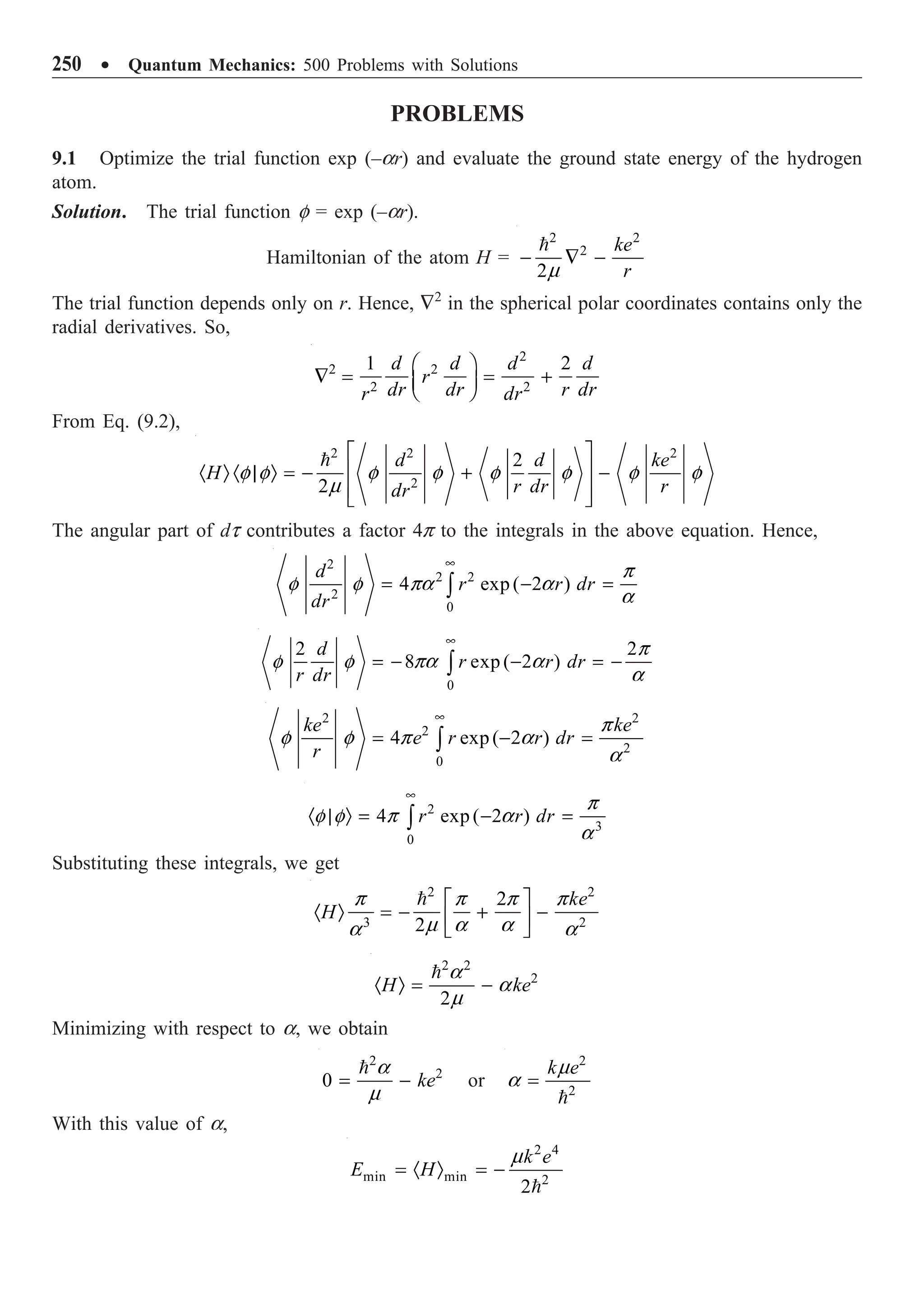
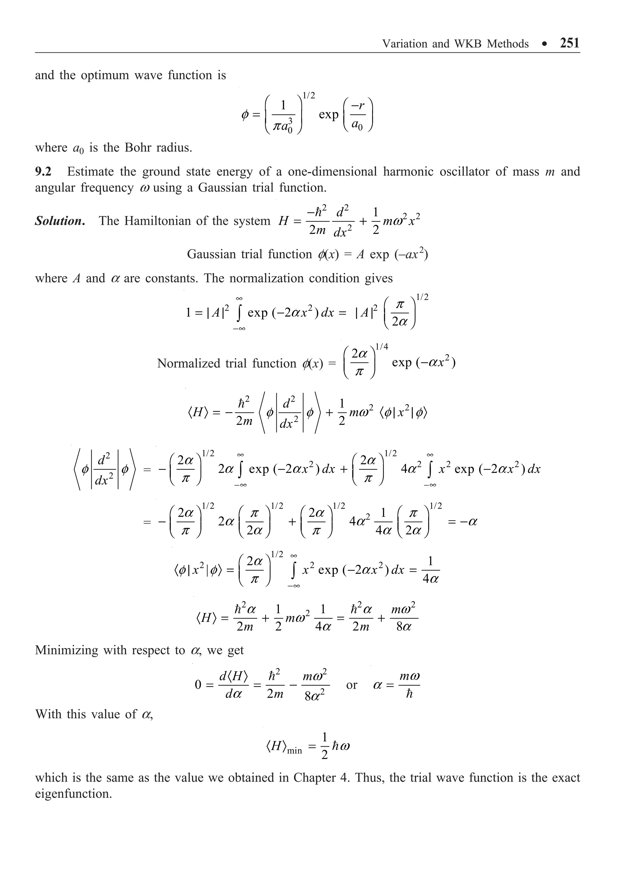
262. 252 ∑ Quantum Mechanics: 500 Problems with Solutions
9.3 The Schrödinger equation of a particle confined to the positive x-axis is
2 2
2
2
d
mgx E
m dx
-
+ =
y
y y
with y(0) = 0, y(x) Æ 0 as x Æ • and E is the energy eigenvalue. Use the trial function
x exp (–ax) and obtain the best value of the parameter a.
Solution.
Hamiltonian H =
2 2
2
2
d
mgx
m dx
-
+
Trial function f(x) = x exp (–ax)
2
3
0
1
exp ( 2 )
4
x ax dx
a
•
· | Ò = - =
Ú
f f
2 2
2
2
d
m dx
-
f f =
2 2 2
2
0 0
exp ( 2 ) exp ( 2 )
2
a
x x dx x x dx
m m
• •
- - -
Ú Ú
a a a
=
2 2 2
4 8 8
ma ma ma
- =
3
4
0
3
| exp ( 2 )
8
mg
mgx mg x x dx
a
•
· | Ò = - =
Ú
f f a
2 4 2 2
3
| | [ /(8 )] (3 /8 ) 3
| 2 2
1/4
H ma mg a a mg
H
m a
a
· Ò +
· Ò = = = +
· Ò
f f
f f
Minimizing ·HÒ with respect to a, we get
2
2
3
0 2
2 2
mg
a
m a
= -
or
1/3
2
2
3
2
m g
a
Ê ˆ
= Á ˜
Ë ¯
which is the best value of the parameter a so that ·HÒ is minimum.
9.4 A particle of mass m moves in the attractive central potential V(r) = –g2
/r3/2
, where g is a
constant. Using the normalized function (k3
/8p)1/2
e–kr/2
as the trial function, estimate an upper bound
to the energy of the lowest state. Given
1
0
!
n ax
n
n
x e dx
a
•
-
+
=
Ú if n is positive and a 0
we have
0
1
2
ax x
xe dx
a a
•
-
=
Ú
Solution. The expectation value of the Hamiltonian
·HÒ = ·f | H | fÒ =
3
2 /2
0
4
8
kr
k
r e
•
-
Ú
p
p
2 2
2 /2
2 3/2
1
2
kr
d d g
r e dr
m dr dr
r r
-
È ˘
Ê ˆ
¥ - -
Í ˙
Á ˜
Ë ¯
Í ˙
Î ˚

263. Variation and WKB Methods ∑ 253
The factor 4p outside the integral comes from the integration of the angular part, and r2
inside the
integral comes from the volume element dt. Then,
2 2
2 /2 /2 /2
2 2
1 2
4
kr kr kr
d d d d k k
r e e e
dr dr r dr r
r dr
- - -
Ê ˆ Ê ˆ
Ê ˆ
= + = -
Á ˜ Á ˜ Á ˜
Ë ¯ Ë ¯ Ë ¯
Hence,
·HÒ =
3 2 2 3
2 /2 /2 2 1/2
0 0
2 2 4 2
kr kr kr
k k k k
r e e dr g r e dr
m r
• •
- - -
Ê ˆ Ê ˆ
- - -
Á ˜ Á ˜
Ë ¯ Ë ¯
Ú Ú
=
2 5 2 4 3 2
2 1/2
0 0 0
16 4 2
kr kr kr
k k k g
r e dr re dr r e dr
m m
• • •
- - -
- + - -
Ú Ú Ú
=
2 5 2 4 3 2
3 2
2 1 1
16 4 2 2
k k k g
m m k k
k k
- + -
p
=
2 2 2 3/2
8 4
k g k
m
-
p
For ·HÒ to be minimum, ∂·HÒ/∂k = 0, i.e.,
2
2 1/2
3
0
4 8
k
g k
m
- =
p
This leads to two values for k, and so
k = 0,
2
1/2
2
3
2
g m
k =
p
The first value can be discarded as it leads to y = 0. Hence the upper bound to the energy of the
lowest state is
2 8 3 2 8 3 2 8 3
min 6 6 2
81 27 27
128 32 128
g m g m g m
H
· Ò = - = -
p p p
9.5 A trial function f differs from an eigenfunction yE so that f = yE + af1, where yE and f1 are
orthonormal and normalized and a 1. Show that ·HÒ differs from E only by a term of order a2
and find this term.
Solution. Given HyE = EyE. We have
·HÒ =
1 1
1 1
( ) ( )
( ) ( )
E E
E E
H
H · + | | + Ò
· | | Ò
=
· | Ò · + | + Ò
y af y af
f f
f f y af y af
=
2
1 1 1 1
2
1 1 1 1
|
E E E E
E E E E
H H H H
· | | Ò + · | | Ò + · | | Ò + · | | Ò
· | Ò + · Ò + · | Ò + · | Ò
y y a y f a f y a f f
y y a y f a f y a f f
Since H is Hermitian,
1 1 0
E E
H E
· | | Ò = · | Ò =
y f y f

264. 254 ∑ Quantum Mechanics: 500 Problems with Solutions
2
2
1 1
1 1
2
| |
| |
1
E H
H E H
+ · Ò
· Ò = = + · Ò
+
a f f
a f f
a
as 1 + a2
@ 1. Hence the result. ·HÒ differs from E by the term 2
1 1
| |
H
· Ò
a f f .
9.6 Evaluate the ground state energy of a harmonic oscillator of mass m and angular frequency w
using the trial function
cos ,
2
( )
0, | |
x
a x a
a
x
x a
Ï Ê ˆ
- £ £
Ô Á ˜
Ë ¯
= Ì
Ô
Ó
p
f
Solution.
2 2
2 2
2
1
2 2
d
m x
m dx
H
H
Ê ˆ
-
+ · | | Ò
Á ˜
Ë ¯
· | | Ò
· Ò = =
· | Ò · | Ò
f f w f f
f f
f f f f
2
cos
2
a
a
x
dx a
a
-
· | Ò = =
Ú
p
f f
2 2 2 2 2 2
2
2 2
cos
2 2 8
8
a
a
d x
dx
m a ma
dx ma -
Ê ˆ
-
= =
Á ˜
Ë ¯
Ú
p p p
f f
2
| |
x
· Ò
f f =
2
2 2 2
1
cos cos
2 2 2
a a a
a a a
x x x
x dx dx x dx
a a
- - -
= +
Ú Ú Ú
p p
=
3 3
3
2 2
2 1 1
2
3 6
a a
a
Ê ˆ
- = -
Á ˜
Ë ¯
p p
·HÒ =
2 2
2 2
2 2
1 1
6
8
m a
ma
Ê ˆ
+ -
Á ˜
Ë ¯
p
w
p
For ·HÒ to be minimum, ∂·HÒ/∂a = 0. Minimizing
2 4
4
2 2 2
6
8 ( 6)
a
m
=
-
p
w p
, we get
1/2
2
min
1 6
0.568
2 3
H
Ê ˆ
-
· Ò = =
Á ˜
Ë ¯
p
w w
9.7 For a particle of mass m moving in the potential,
, 0
( )
, 0
kx x
V x
x
Ï
= Ì
•
Ô
Ó
where k is a constant. Optimize the trial wavefunction f = x exp (–ax), where a is the variable
parameter, and estimate the groundstate energy of the system.

265. Variation and WKB Methods ∑ 255
Solution. In the region x 0, the wave function is zero since V(x) = •. The Hamiltonian of the
system
2 2
2
,
2
d
H kx
m dx
= - +
x 0,
|
H
H
· | Ò
· Ò =
· | Ò
f f
f f
2 2
3
0
1
4
ax
x e dx
a
•
-
· | Ò = =
Ú
f f
2
2
2
( ) 2
ax ax ax
d
xe a xe ae
dx
- - -
= -
2
2
0
( )
ax ax
d
xe xe dx
dx
•
- -
Ú =
2 2 2 2
0 0
2
ax ax
a x e dx a xe dx
• •
- -
-
Ú Ú
=
1 1 1
4 2 4
a a a
- = -
0
( )
ax ax
xe kx xe dx
•
- -
Ú =
3 2
4
0
3
8
ax k
k x e dx
a
•
-
=
Ú
·HÒ =
2 2 2
3
4
3 3
4
8 2 2
8
k a k
a
ma m a
a
Ê ˆ
+ = +
Á ˜
Ë ¯
Minimizing with respect to a, we get
1/3
2
3
,
2
km
a
Ê ˆ
= Á ˜
Ë ¯
1/3
2 2
min
9 2
4 3
k
H
m
Ê ˆ
· Ò = Á ˜
Ë ¯
9.8 The Hamiltonian of a particle of mass m is
2 2
4
2
2
d
H bx
m dx
= - +
where b is a constant. Use the trial function f(x) = Ae–a2x2
, where a is the variable parameter, to
evaluate the energy of the ground state. Given
1/2
2
0
1
exp ( )
2
x dx
•
Ê ˆ
- = Á ˜
Ë ¯
Ú
p
a
a
2 2
3/2
0
1
exp ( )
4
x x dx
•
- =
Ú
p
a
a
4 2
5/2
0
3 1
exp ( )
8
x x dx
•
- =
Ú
p
a
a

266. 256 ∑ Quantum Mechanics: 500 Problems with Solutions
Solution. The Hamiltonian H and the trial function f(x) are
2 2
4
2
2
d
H bx
m dx
= - +
f(x) = Aee–a2x2
The normalization condition gives
1 =
2 2
2 2 x
A e dx
•
-
-•
| | Ú
a
1 =
1/2
2
2
2
A
Ê ˆ
| | Á ˜
Ë ¯
p
a
or
1/2
2
2 2
A
Ê ˆ
| | Á ˜
Ë ¯
a
p
·HÒ =
2 2
4
2
2
d
H bx
m dx
· | | Ò = - +
f f f f
=
2 2 2 2 2 2
2 2
2 2 2 2 4 2 2 2 4 2
| 2 | 4 |
2 2
x x x
A e dx A x e dx b A x e dx
m m
• • •
- - -
-• -• -•
| - | + |
Ú Ú Ú
a a a
a a
=
2 2 2 2
4
3 1
2 16
b
m m
- +
a a
a
=
2 2
4
3
2 16
b
m
+
a
a
Minimizing ·HÒ with respect to a, we have
2
5
3
0
4
H b
m
∂· Ò
= = -
∂
a
a a
1/3
2
2
3
4
bm
Ê ˆ
= Á ˜
Ë ¯
a
Substituting this value of a, we get
1/3 1/3
1/3 4/3
4 4
min 2 2
3 3 3
4 4 4
b b
H
m m
Ê ˆ Ê ˆ
Ê ˆ Ê ˆ
· Ò = =
Á ˜ Á ˜
Á ˜ Á ˜
Ë ¯ Ë ¯
Ë ¯ Ë ¯
9.9 An anharmonic oscillator is described by the Hamiltonian
2 2
4
2
2
d
H Ax
m dx
= - +
Determine its ground state energy by selecting
1/2 2 2
1/4
exp
2
x
Ê ˆ
-
= Á ˜
Ë ¯
l l
y
p
l being a variable parameter as the variational trial wave function.

267. Variation and WKB Methods ∑ 257
Solution. With the trial function y, the expectation value of H is
2 2 2 2
2 2
1/2 /2 4 /2
2
2
x x
d
H e Ax e dx
m dx
•
- - -
-•
Ê ˆ
· Ò = - +
Á ˜
Ë ¯
Ú
l l
lp
Using the values of the first three integrals from the Appendix, we obtain
2 2
4
3
4 4
A
H
m
· Ò = +
l
l
Minimizing ·HÒ with respect the variable parameter l, we get
0 =
2
5
3
2
H A
m
∂ · Ò
= -
∂
l
l l
l =
1/6
2
6mA
Ê ˆ
Á ˜
Ë ¯
Substituting this value of l, we obtain
·HÒ =
2/3
1/3
2 2
2
6 3
4 4 6
mA A
m mA
Ê ˆ
Ê ˆ
+
Á ˜ Á ˜
Ë ¯ Ë ¯
=
2/3 2/3
1/3 2 1/3 2
1/3 1/3
3 3
2 2 2 2
A A
m m
Ê ˆ Ê ˆ
+
Á ˜ Á ˜
Ë ¯ Ë ¯
=
2/3 2/3
4/3 2
1/3 1/3
3
1.082
4 2 2
A A
m m
Ê ˆ Ê ˆ
= Á ˜
Á ˜ Ë ¯
Ë ¯
It may be noted that numerical integration gives a coefficient of 1.08, illustrating the usefulness of
the variation method. It may also be noted that perturbation technique is not possible as there is no
way to split H into an unperturbed part and a perturbed part.
9.10 The Hamiltonian of a system is given by
2 2
2
( )
2
d
H a x
m dx
-
= -
d
where a is a constant and d(x) is Dirac’s delta function. Estimate the ground state energy of the
system using a Gaussian trial function.
Solution. The normalized Gaussian trial function is given by f(x) = (2b/p)1/4
exp (–bx2
). Then,
·HÒ =
2 2
2
( )
2
d
a x
m dx
- - · | | Ò
f f f d f
2
2
d
dx
f f =
1/2 1/2
2 2 2 2
2 2
2 exp ( 2 ) 4 exp ( 2 )
b b
b bx dx b x bx dx
• •
-• -•
Ê ˆ Ê ˆ
- + -
Á ˜ Á ˜
Ë ¯ Ë ¯
Ú Ú
p p
=
1/2 1/2 1/2 1/2
2
2 2 1
2 4
2 4 2
b b
b b b
b b b
Ê ˆ Ê ˆ Ê ˆ Ê ˆ
- + = -
Á ˜ Á ˜ Á ˜ Á ˜
Ë ¯ Ë ¯ Ë ¯ Ë ¯
p p
p p

268. 258 ∑ Quantum Mechanics: 500 Problems with Solutions
( )
x
· | | Ò
f d f =
1/2
2
2
( ) exp ( 2 )
b
x bx dx
•
-•
Ê ˆ
-
Á ˜
Ë ¯ Ú d
p
=
1/2 1/2
2
0
2 2
exp ( 2 ) x
b b
bx =
Ê ˆ Ê ˆ
- | =
Á ˜ Á ˜
Ë ¯ Ë ¯
p p
·HÒ =
1/2
2
2
2
b b
a
m
Ê ˆ
- Á ˜
Ë ¯
p
Minimizing ·HÒ with respect to b, we get
2 2
4
2m a
b =
p
or
2
min 2
ma
H
· Ò = -
p
9.11 Evaluate the ground state energy of hydrogen atom using a Gaussian trial function. Given
1/2
2 2
2 1 1/2
0
(2 ) !
exp ( )
2 !
n
n n
n
x x dx
n
•
+ +
- =
Ú
p
l
l
2 1 2
1
0
!
exp ( )
2
n
n
n
x x dx
•
+
+
- =
Ú l
l
Solution.
Hamiltonian H =
2 2
2
2
e
r
- — -
m
The Gaussian trial function f(r) = exp (–br2
), where b is the variable parameter. Since f depends
only on r, only the radial derivative exists in —2
. However, the angular integration of dt gives a factor
of 4p. Hence,
·HÒ =
2 2 2 2
2
2
2 2
d d e
m m r dr r
dr
Ê ˆ Ê ˆ
- - -
Á ˜ Á ˜
Ë ¯ Ë ¯
· | Ò
f f f f f f
f f
· | Ò
f f =
3/2
2 2
0
4 exp ( 2 )
2
r br dr
b
•
Ê ˆ
- = Á ˜
Ë ¯
Ú
p
p
2
2
d
dr
f f =
2 2
2 2 2 4 2
0 0
4 ( 2 ) 4 4
br br
b r e dr b r e dr
• •
- -
- + ¥
Ú Ú
p p
=
3/2
3/2 3/2
1/2 5/2
6
2
(2 ) (2 )
b
b
b b
Ê ˆ
- + = Á ˜
Ë ¯
p p p
2 d
r dr
f f =
2
3/2
2 2
0
16 ( 4 )
2
br
b r e dr b
b
•
- Ê ˆ
- = -
Á ˜
Ë ¯
Ú
p
p

269. Variation and WKB Methods ∑ 259
2
2 2
2 2
0
4 br
e e
e re dr
r b
•
-
= =
Ú
p
f f p
1/2
2
2 1/2
3 2
2
2
b
H e b
Ê ˆ
· Ò = + Á ˜
Ë ¯
m p
Minimizing ·HÒ with respect to b given by
2 4
4
8
9
e
b =
m
p
, we get
4
min 2
8
11.59 eV
3 2
e
H
Ê ˆ
-
· Ò = = -
Á ˜
Ë ¯
m
p
9.12 A particle of mass m is moving in a one-dimensional box defined by the potential V = 0,
0 £ x £ a and V = • otherwise. Estimate the ground state energy using the trial function y(x) =
Ax(a – x), 0 £ x a.
Solution. The normalization condition gives
2 2 2
0
( ) 1
a
A x a x
· | Ò = - =
Ú
y y
2 2 2 3 4
0 0 0
2 1
a a a
A a x dx a x dx x dx
È ˘
- + =
Í ˙
Í ˙
Î ˚
Ú Ú Ú
2 5
1
30
A a
= or 5
30
A
a
=
The normalized trial function is
5
30
( ) ( ),
x x a x
a
= -
y 0 £ x £ a
The Hamiltonian of the system is given by
H =
2 2
2
2
d
m dx
-
·HÒ =
2 2
2 2
5 2
0
30
( ) ( )
2
a
d
ax x ax x dx
m a dx
- - -
Ú
=
2 2 2
2
5 2 2
0
30 5 10
( )
2
a
ax x dx
ma ma ma
- = =
Ú
which is the ground state energy with the trial function. It may be noted that the exact ground state
energy is p2
2
/(2ma2
), which is very close to the one obtained here.

270. 260 ∑ Quantum Mechanics: 500 Problems with Solutions
9.13 Evaluate, by the variation method, the energy of the first excited state of a linear harmonic
oscillator using the trial function
f = Nx exp (–lx2
)
where is the l variable parameter.
Solution. The Hamiltonian
2 2
2
2
1
2 2
d
H kx
m dx
= - +
The trial function
f = Nx exp (–lx2
)
where l is the variable parameter. The normalization condition gives
1 =
2
2 2 2 2
3/2
1
2
4 (2 )
x
N x e dx N
•
-
-•
= ¥ ¥
Ú
l p
l
N2 =
5/2 3/2
1/2
2 l
p
·HÒ =
2 2
2
2
1
2 2
d
k x
m dx
- + · | | Ò
f f f f
2
2
d
dx
f f =
2
2 2 2 4 2
( 6 4 ) x
N x x e dx
•
-
-•
- +
Ú
l
l l
=
1/2 1/2 1/2
2 2
3/2 1/2 5/2 1/2 5/2 1/2
3 3 3
2 2 2
N N
Ê ˆ
- + = -
Á ˜
Ë ¯
p p p
l l l
Substituting the value of N2
, we get
2 1/2 5/2 3/2
2 5/2 1/2 1/2
3 2
3
2
d
dx
= - = -
p l
f f l
l p
2
1/2
2 2 4 2 2
5/2
3 3
4
4 (2 )
x
x N x e dx N
•
-
-•
· | | Ò = = =
Ú
l p
f f
l
l
Substituting these values, we obtain
2 2
1 3 3 3
( 3 )
2 2 4 2 8
k
H k
m m
Ê ˆ
· Ò = - - + ¥ = +
Á ˜
Ë ¯
l
l
l l
Minimizing ·HÒ with respect to l, we obtain
2
2
3 3
0
2 8
k
m
- =
l
or
2
km
=
l

271. Variation and WKB Methods ∑ 261
Substituting this value of l in ·HÒ, we get
min
3 3
2 2
k
H
m
· Ò = =
w
9.14 Estimate the ground state energy of helium atom by taking the product of two normalized
hydrogenic ground state wave functions as the trial wave function, the nuclear charge Z¢e being the
variable parameter. Assume that the expectation value of the interelectronic repulsion term is
(5/4) ZWH, WH = 13.6 eV.
Solution. The Hamiltonian of the helium atom having a nuclear charge Ze (Fig. 9.1) is given by
2 2 2 2 2
2 2
1 2
1 2 12
2 2
kZe kZe ke
H
m r m r r
Ê ˆ Ê ˆ
= - — - + - — - +
Á ˜ Á ˜
Ë ¯ Ë ¯
(i)
where
0
1
4
k =
pe
r12
Ze
r1
r2
–e
–e
1
2
Fig. 9.1 The helium atom.
In terms of the variable parameter Z¢e, it is convenient to write the Hamiltonian as
2 2 2 2 2
2 2 2
1 2
1 2 1 2 12
1 1
( )
2 2
kZ e kZ e ke
H Z Z ke
m r m r r r r
Ê ˆ Ê ˆ
¢ ¢ Ê ˆ
¢
= - — - + - — - + - + +
Á ˜ Á ˜ Á ˜
Ë ¯
Ë ¯ Ë ¯
(ii)
The product of the two normalized hydrogenic ground state wave functions is
3
1 1 2 2 1 2
3
0
0
( ) ( ) exp ( )
Z Z
r r r r
a
a
¢ ¢
È ˘
= = - +
Í ˙
Î ˚
y y y
p
(iii)
where y1(r1) and y2(r2) are the normalized hydrogenic wave functions with Z replaced by Z¢. The
expectation value of H with the trial wave function, as seen from Eq. (iii), is
·HÒ =
2 2 2 2
2 2
1 1 1 2 2 2
1 2
2 2
kZ e kZ e
m r m r
¢ ¢
- — - + - — -
y y y y
2 2 2
1 1 2 2 1 2 1 2
1 2 12
( ) ( )
ke ke ke
Z Z Z Z
r r r
¢ ¢
+ - + - +
y y y y y y y y

272. 262 ∑ Quantum Mechanics: 500 Problems with Solutions
The value of the first and second terms are equal and each is –Z¢2
WH, where WH = k2
me4
/22
.
2
1 1
1
ke
r
y y =
2
3 2
1
1 1 1 1 1
3
0
0 0 0
0
2
sin exp
Z r
Z ke
d d r dr
a
a
•
¢
¢ Ê ˆ
-
Á ˜
Ë ¯
Ú Ú Ú
p p
f q f
p
=
3 2
3 2
0 0
1
4
(2 / )
Z ke
a Z a
¢
¢
p
p
=
2
0
2 H
Z ke
Z W
a
¢
¢
= (iv)
where the value of a0 is substituted. Given
2
1 2 1 2
12
5
4 H
ke
Z W
r
¢
=
y y y y (v)
Summing up, we have
2 5
2 4( )
4
H H H
H Z W Z Z Z W Z W
¢ ¢ ¢ ¢
· Ò = - + - + (vi)
Minimizing ·HÒ with respect to Z¢, we get
5
4 8 4 0
4
H H H H
Z W Z W ZW W
¢ ¢
- + - + =
5
16
Z Z
¢ = - (vii)
With this value of Z¢, Eq. (vi) gives
2
5
2
16 H
E H Z W
Ê ˆ
= · Ò = - -
Á ˜
Ë ¯
Substitution of WH = 13.6 eV leads to a ground state energy of –77.46 eV.
9.15 The attractive short range force between the nuclear particles in a deuteron is described by the
Yukawa potential
/
0
( )
/
r
e
V r V
r
-
= -
b
b
where V0 and b are constants. Estimate the ground state energy of the system using the trial function
1/2
3
/
3
r
e-
Ê ˆ
= Á ˜
Ë ¯
a b
a
f
pb
where a is a variable parameter.
Solution. The Hamiltonian for the ground state is
2
2
( )
2
H V r
= - — +
m
(i)

273. Variation and WKB Methods ∑ 263
As the trial function depends only on r, we need to consider only the radial derivative in —2
:
2
2 2
2 2
1 2
d d d d
r
dr dr r dr
r dr
Ê ˆ
— = = +
Á ˜
Ë ¯
(ii)
Consequently,
2 2 2
2
2
2 2
d
H H V
r
dx
· Ò = · | | Ò = - - + · | | Ò
f f f f f f f f
m m
(iii)
While evaluating integrals in Eq. (iii), the factor dt gives the angular contribution 4p. Using the
integrals in the Appendix, we get
2
2
d
dx
f f =
3 2
2
3 2
0
2
4 exp
r
r dr
•
Ê ˆ
-
Á ˜
Ë ¯
Ú
a a a
p
b
pb b
=
3 2 2
3 2 3 2
2
4
(2 / )
=
a a a
p
pb b a b b
(iv)
2
r
f f =
3
3
0
8 2
exp
r
r dr
•
Ê ˆ Ê ˆ
- -
Á ˜ Á ˜
Ë ¯ Ë ¯
Ú
a pa a
b b
pb
=
4 2 2
4 2 2
8 2
4
- = -
a b a
b a b
(v)
( )
V r
· | | Ò
f f =
3
0
3
0
2 1
( 4 ) exp
V r r dr
•
+
Ê ˆ
- -
Á ˜
Ë ¯
Ú
a a
pb
b
pb
=
3
3 2
0
0
3 2 2
4
( 4 )
(2 1) (2 1)
V
V
- = -
+ +
a
a b
p b
pb a a
(vi)
Adding all the contributions, we here
·HÒ =
3
2 2 2 2
0
2 2 2
4
2
2 2 (2 1)
V
a
- + -
+
a
a a
m b mb
=
3
2 2
0
2 2
4
2 (2 1)
V
a
-
+
a
a
m b
(vii)
Minimizing with respect to a, we obtain
0 =
2
2
0
2 3
4 (2 3)
(2 1)
V
a
+
-
+
a a
a
mb
2
0
2 3
2 (2 3)
2 (2 1)
V +
=
+
a a
mb a
(viii)

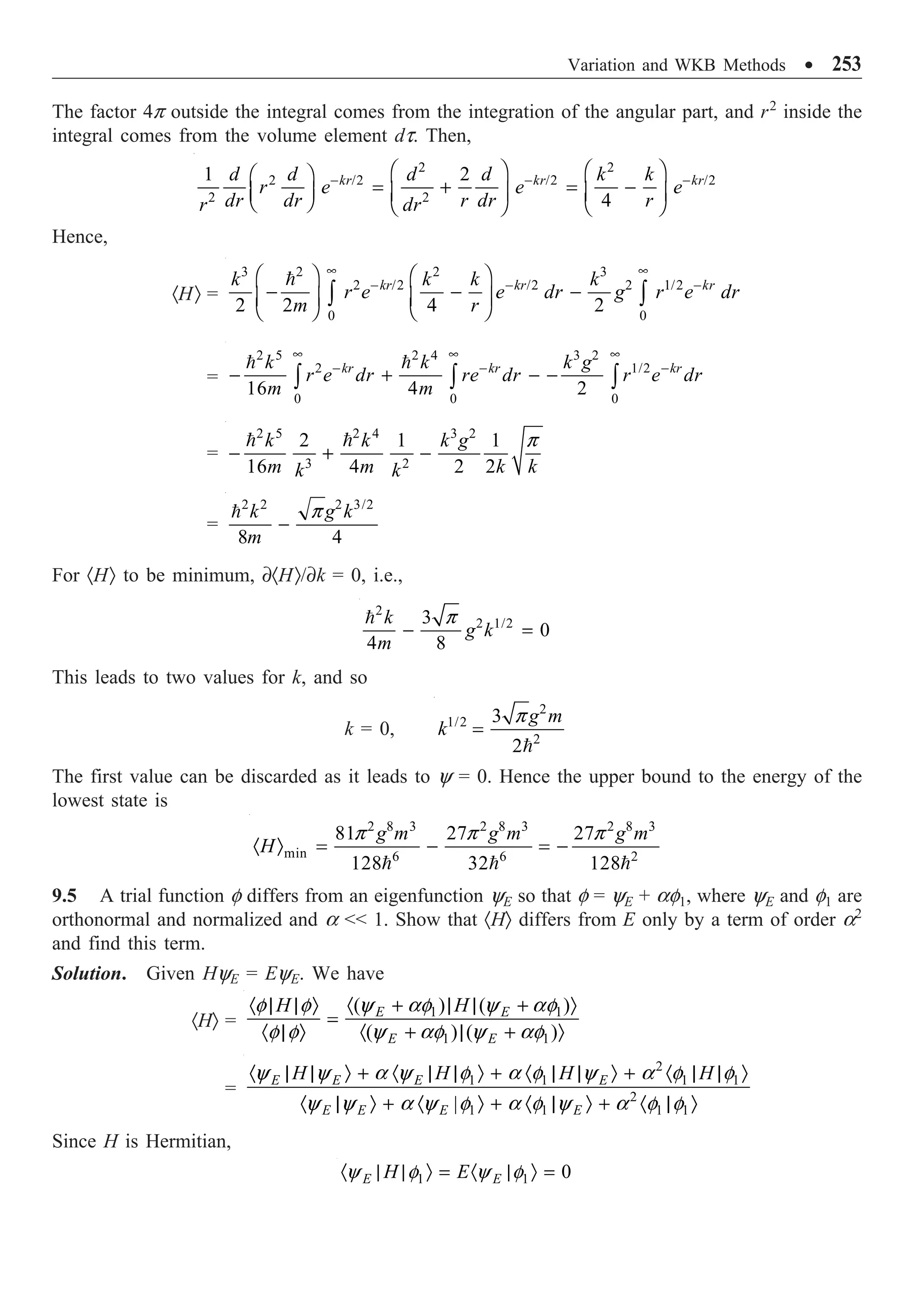
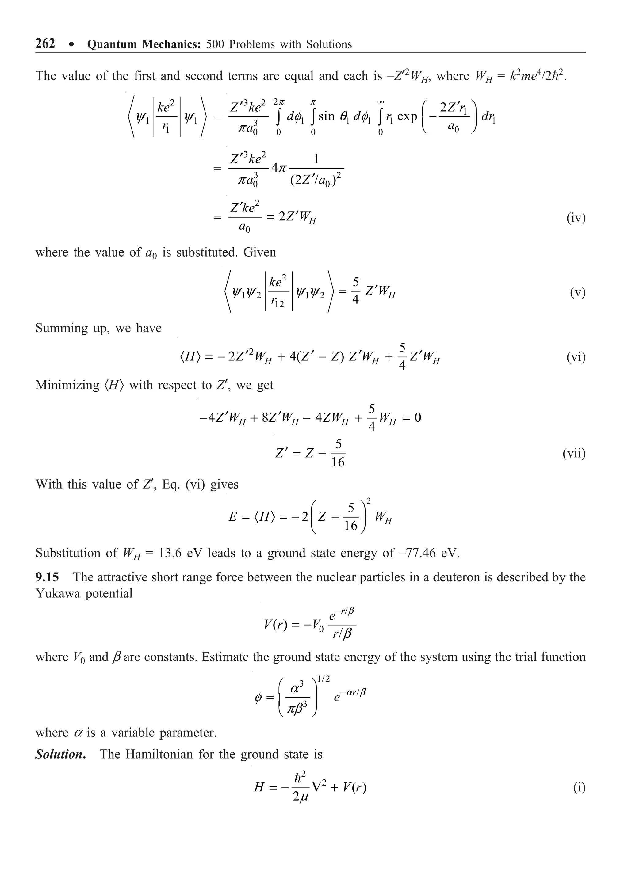
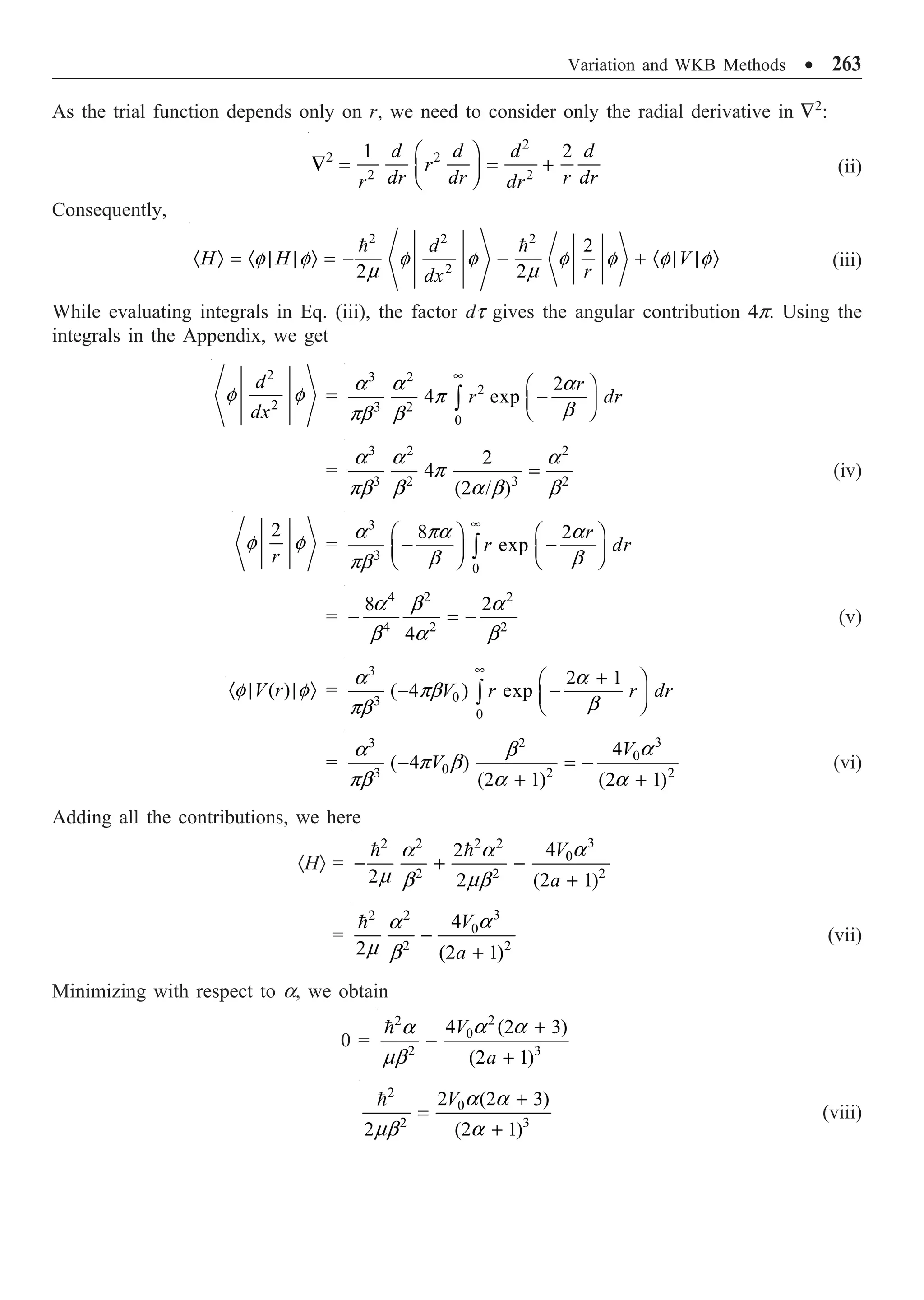
274. 264 ∑ Quantum Mechanics: 500 Problems with Solutions
Repalcing 2
/2mb2
in Eq. (vii) using Eq. (viii), we get
·HÒ =
3 3
0 0
3 2
2 (2 3) 4
(2 1) (2 1)
V V
+
-
+ +
a a a
a a
=
3
0
3
2
[(2 3) 2(2 1)]
(2 1)
V
+ - +
+
a
a a
a
E =
3
0
2 (2 1)
(2 1)
V -
+
a a
a
where a is given by Eq. (viii).
9.16 Consider a particle having momentum p moving inside the one-dimensional potential well
shown in Fig. 9.2. If E V(x), show by the WKB method, that
2
1
1
2 ,
2
x
x
p dx n h
Ê ˆ
= +
Á ˜
Ë ¯
Ú n = 0, 1, 2, º
V(x)
x1 x2 x
E = V(x1)
Region 1 Region 2 Region 3
E = V(x2)
Fig. 9.2 A potential well with linear turning points at x1 and x2.
Solution. Classically, the particle will oscillate back and forth between the turning points x1 and
x2. Quantum mechanically, the particles can penetrate into regions 1 and 2. The wave functions in
regions 1 and 2 are exponentially decreasing. When we move from region 1 to region 2, the barrier
is to the left of the turning point and, when we move from region 2 to region 3, the barrier is to the
right of the turning point. The wave function in region 1 is
1
2
1
1
exp ,
x
x
dx
r
Ê ˆ
= -
Á ˜
Ë ¯
Ú
y g 2
2
2 [ ( ) ]
m V x E
-
=
g (i)
Applying Eq. (9.8), we get
1
2
2
2
cos ,
4
x
x
k dx
k
Ê ˆ
= -
Á ˜
Ë ¯
Ú
p
y 2
2
2 [ ( )]
m E V x
k
-
=
(ii)

275. Variation and WKB Methods ∑ 265
The wave function that connects region 2 with the decreasing potential of region 3 being of the type
2
1
cos
4
x
x
k dx
Ê ˆ
-
Á ˜
Ë ¯
Ú
p
Hence, Eq. (ii) should be modified as
2
1 2
2
2
cos
4
x x
x x
k dx k dx
k
Ê ˆ
= + -
Á ˜
Ë ¯
Ú Ú
p
y (iii)
Since cos (–q) = cos q and sin (–q) = –sin q, Eq. (iii) can be rewritten as
y2 =
2 2 2 2
1 1
2 2
cos cos sin sin
4 4
x x x x
x x x x
k dx k dx k dx k dx
k k
Ê ˆ Ê ˆ
Ê ˆ Ê ˆ
+ + +
Á ˜ Á ˜
Á ˜ Á ˜
Ë ¯ Ë ¯
Ë ¯ Ë ¯
Ú Ú Ú Ú
p p
=
2 2 2 2
1 1
2 2
cos sin sin cos
4 4
x x x x
x x x x
k dx k dx k dx k dx
k k
Ê ˆ Ê ˆ
Ê ˆ Ê ˆ
- + -
Á ˜ Á ˜
Á ˜ Á ˜
Ë ¯ Ë ¯
Ë ¯ Ë ¯
Ú Ú Ú Ú
p p
(iv)
Comparison of Eqs. (iv) and (9.7) shows that the second term of Eq. (iv) is the one that connects
with the decreasing exponential of region 3, while the first term connects with the increasing
exponential. Since an increasing exponential in region 3 is not acceptable, the first term has to be
zero. This is possible if
2
1
cos 0
x
x
k dx =
Ú or
2
1
1
,
2
x
x
k dx n
Ê ˆ
= +
Á ˜
Ë ¯
Ú p n = 0, 1, 2, º (v)
Substituting the value of k, we get
2
1
1/2
1/2
2
2 1
[ ( )] ,
2
x
x
m
E V x dx n
Ê ˆ Ê ˆ
- = +
Á ˜ Á ˜
Ë ¯ Ë ¯
Ú
p n = 0, 1, 2, º (vi)
which gives the allowed energy value. Classically, since the linear momentum p = [2m (E – V)]1/2
,
Eq. (vi) can be rewritten as
2
1
1
2 ,
2
x
x
p dx n h
Ê ˆ
= +
Á ˜
Ë ¯
Ú n = 0, 1, 2, º (vii)
The LHS is the value of the integral over a complete cycle.
9.17 Obtain the energy values of harmonic oscillator by the WKB method.
Solution. The classical turning points of the oscillator are those points at which the potential V(x)
= E, i.e., 1/2mw2
x2
= E or x1 = –(2E/mw2
)1/2
and x2 = (2E/mw2
)1/2
. For a particle constrained to move
between classical turning points x1 and x2 in a potential well, the energies can be obtained from the
condition (vii) of Problem 9.16. We then have
E =
2
2 2
1
2 2
p
m x
m
+ w or
1/2
2 2
1
2
2
p m E m x
È ˘
Ê ˆ
= -
Í ˙
Á ˜
Ë ¯
Î ˚
w

276. 266 ∑ Quantum Mechanics: 500 Problems with Solutions
Substituting this value of p in Eq. (vii) of Problem 9.16, we get
2
1
1/2
2 2
1 1
2 ,
2 2
x
x
m E m x dx n
È ˘
Ê ˆ Ê ˆ
- = +
Í ˙
Á ˜ Á ˜
Ë ¯ Ë ¯
Î ˚
Ú
w p n = 0, 1, 2, º
Writing sin q = (mw2
/2E)1/2
x, the above integral reduces to
1/2
/2
1/2 2
2
/2
2 1
(2 ) cos
2
E
mE d n
m
-
Ê ˆ Ê ˆ
= +
Á ˜ Á ˜
Ë ¯ Ë ¯
Ú
p
p
q q p
w
/2
2
/2
2 1
cos
2
E
d n
-
Ê ˆ Ê ˆ
= +
Á ˜ Á ˜
Ë ¯ Ë ¯
Ú
p
p
q q p
w
2 1
2 2
E
n
Ê ˆ
¥ = +
Á ˜
Ë ¯
p
p
w
or
1
2
E n
Ê ˆ
= +
Á ˜
Ë ¯
w
9.18 Solve the following one-dimensional infinite potential well:
V(x) = 0 for –a x a; V(x) = • for | x | a
using the WKB method and compare it with the exact solution.
Solution. V(x) = 0 for –a x a and V(x) = • for | x | a. The turning points are x1 = –a and
x2 = a. The allowed energies can be obtained using the relation
1
,
2
a
a
k dx n
-
Ê ˆ
= +
Á ˜
Ë ¯
Ú p 2
2
2
,
mE
k =
n = 0, 1, 2, º
1/2
2
2 1
2
a
a
mE
dx n
-
Ê ˆ Ê ˆ
= +
Á ˜ Á ˜
Ë ¯ Ë ¯
Ú
p
2 2 2
2
[ (1/2) ]
,
8
n
n
E
ma
+
=
p
n = 0, 1, 2, º
The exact solution gives
2 2 2
2
,
8
n
n
E
ma
=
p
n = 1, 2, 3, º
The WKB solution has n + (1/2) in place of n. Another major difference is in the allowed values
of n.
9.19 Estimate the energy levels of a particle moving in the potential
V(x) =
, 0
, 0
x
Ax x
•
Ï
Ì
Ô
Ó
A being a constant.
Solution. The classical turning points are at x1 = 0 and at x2 = E/A. Now,
2
1
1
,
2
x
x
k dx n
Ê ˆ
= +
Á ˜
Ë ¯
Ú p 2
2
2
( )
m
k E V
= -

277. Variation and WKB Methods ∑ 267
In the given case,
1/2
1/2
2
2
( )
m
k E Ax
Ê ˆ
= -
Á ˜
Ë ¯
1/2 /
1/2
2
0
2 1
( )
2
E A
m
E Ax dx n
Ê ˆ Ê ˆ
- = +
Á ˜ Á ˜
Ë ¯ Ë ¯
Ú
p
/
1/2 3/2
2
2 ( ) 1
3/2 2
E A
m E Ax
n
A
È ˘
-
Ê ˆ Ê ˆ
- = +
Í ˙
Á ˜ Á ˜
Ë ¯ Ë ¯
Í ˙
Î ˚
p
1/3 2/3
2
3 (2 1)
,
2 4
n
A n
E
m
Ê ˆ +
È ˘
= Á ˜ Í ˙
Ë ¯ Î ˚
p
n = 0, 1, 2, º
9.20 Find the energy levels of a particle moving in the potential V(x) = V0 | x |, V0 being a positive
constant.
Solution. The turning points are given by
E = V0 | x | or | x | = E/V0 or x = ±E/V0
2
1
1
,
2
x
x
k dx n
Ê ˆ
= +
Á ˜
Ë ¯
Ú p
1/2
1/2
0
2
2
( )
m
k E V x
Ê ˆ
= - | |
Á ˜
Ë ¯
0
0
1/2 /
1/2
0
2
/
2 1
( )
2
E V
E V
m
E V x dx n
-
Ê ˆ Ê ˆ
- | | = +
Á ˜ Á ˜
Ë ¯ Ë ¯
Ú
p
As the integrand is even,
0
1/2 /
1/2
0
2
0
2 1
2 ( )
2
E V
m
E V x dx n
Ê ˆ Ê ˆ
- | | = +
Á ˜ Á ˜
Ë ¯ Ë ¯
Ú
p
0
/
1/2
0
2
0 0
2 1
2
3 /2 2
E V
E V x
m
n
V
- | |
È ˘
Ê ˆ Ê ˆ
= +
Á ˜ Á ˜
Í ˙
-
Ë ¯ Ë ¯
Î ˚
p
1/3
2/3 2
0
3 1
,
4 2 2
n
E n V
m
Ê ˆ
È ˘
Ê ˆ
= +
Í ˙
Á ˜ Á ˜
Ë ¯ Ë ¯
Î ˚
p n = 0, 1, 2, 3, º
9.21 Consider a particle of mass m moving in a spherically symmetric potential V = kr, k being a
positive constant. Estimate the ground state energy using a trial function of the type f = exp (–ar),
where a is the variable parameter.
Solution. The Hamiltonian operator
2
2
2
H kr
m
= - — +

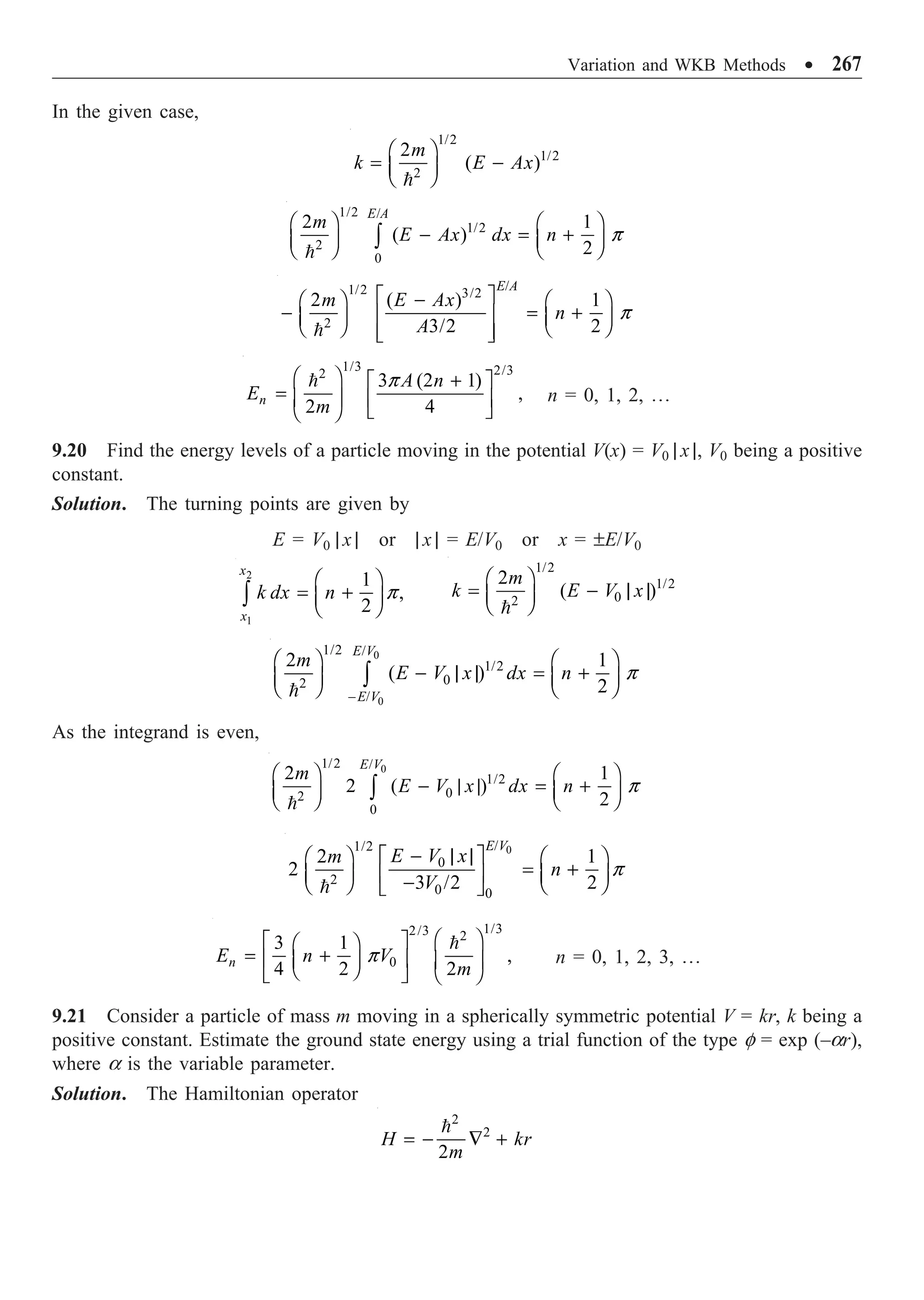
278. 268 ∑ Quantum Mechanics: 500 Problems with Solutions
As the trial wave function is not normalized,
,
H
H
· | | Ò
· Ò =
· | Ò
f f
f f
f = e–ar
2 2
3 3
0
2! 1
(2 ) 4
r
e r dr
•
-
· | Ò = = =
Ú
a
f f
a a
(see Appendix). Now,
·f | H | fÒ =
2
2 2 3 2
2
0 0
1
2
r r r
d d
e r e r dr k r e dr
m dr dr
r
• •
- - -
È ˘
Ê ˆ
- +
Í ˙
Á ˜
Ë ¯
Î ˚
Ú Ú
a a a
=
2 2 2
2 2 2 3 2
0 0 0
2
r r r
r e dr re dr k r e dr
m m
• • •
- - -
- + +
Ú Ú Ú
a a a
a a
Using the standard integral in the Appendix, we get
·f | H | fÒ =
2 2 2
3 2 4
2! 1 3 !
2 (2 ) (2 ) (2 )
k
m m
- + +
a a
a a a
=
2
4
3
8 8
k
m
+
a a
·HÒ =
2 2
3
2 2
H k
m
· | | Ò
= +
· | Ò
f f a
f f a
For ·HÒ to be minimum, it is necessary that
0
H
∂· Ò
=
∂a
2
2
3
0
2
k
m
- =
a
a
or
1/3
2
3
2
km
Ê ˆ
= Á ˜
Ë ¯
a
With this value of a, the ground state energy
2/3 1/3
2/3
2 2 2 2
2
3 3 2 3 9
2 2 3 2 4
2
mk k k
E
m km m
Ê ˆ Ê ˆ
Ê ˆ
= + =
Á ˜ Á ˜ Á ˜
Ë ¯ Ë ¯ Ë ¯
9.22 Using the WKB method, calculate the transmission coefficient for the potential barrier
0 1 ,
( )
0,
x
V x
V x
x
l
l
l
Ï | |
Ê ˆ
- | |
Ô Á ˜
Ë ¯
= Ì
Ô | |
Ó
Solution. The transmission coefficient
2
1
exp 2 ,
x
x
T dx
Ê ˆ
= -
Á ˜
Ë ¯
Ú l 2
2
2
[ ( ) ]
m
V x E
= -
l

279. Variation and WKB Methods ∑ 269
where x1 and x2 are the turning points. At the turning points,
0
( ) 1
x
E V x V
| |
Ê ˆ
= = -
Á ˜
Ë ¯
l
or
0
1
E x
V
| |
= -
l
0
0
V E
x
V
-
Ê ˆ
| | = Á ˜
Ë ¯
l or
0
0
V E
x
V
-
Ê ˆ
= ± Á ˜
Ë ¯
l
0
1
0
V E
x
V
-
Ê ˆ
= - Á ˜
Ë ¯
l ,
0
2
0
V E
x
V
-
Ê ˆ
= Á ˜
Ë ¯
l
2
1
2
x
x
dx
- Ú g =
2
1
1/2
0
0
2
2
2
x
x
V x
m
V E dx
Ê ˆ
- - -
Á ˜
Ë ¯
Ú
l
=
2
1
3/2
0
0
0
2 2 2
3
x
x
V x
m
V E
V
È ˘
Ê ˆ Ê ˆ
Ê ˆ
Í ˙
- - - -
Á ˜ Á ˜ Á ˜
Ë ¯ Ë ¯ Ë ¯
Í ˙
Î ˚
l
l
= 3/2
0
0
16
( )
3
m
V E
V
- -
l
T = 3/2
0
0
16
exp ( )
3
m
V E
V
È ˘
- -
Í ˙
Í ˙
Î ˚
l
9.23 Use the WKB method to calculate the transmission coefficient for the potential barrier
V(x) =
0 , 0
0, 0
V ax x
x
-
Ï
Ì
Ô
Ó
Solution. The transmission coefficient
2
1
exp 2 ,
x
x
T dx
Ê ˆ
= -
Á ˜
Ë ¯
Ú g 2
2
2
[ ( ) ]
m
V x E
= -
g
From the value of V(x), it is clear that the turning point x1 = 0. To get the other turning point, it is
necessary that
E = V(x) = V0 – ax2
x2 = 0
V E
a
-
g = 1/2
0
2
( )
m
V ax E
- -

280. 270 ∑ Quantum Mechanics: 500 Problems with Solutions
2
1
2
x
x
dx
- Ú g =
2
1/2
0
0
2
2 ( )
x
m
V E ax dx
- - -
Ú
=
2
3/2
0
0
2 2 1
2 ( )
3
x
m
V E ax
a
Ê ˆ È ˘
- - - -
Á ˜ Î ˚
Ë ¯
= 3/2 3/2
0 0
4 2
[( ) ( ) ]
3
m
V E ax V E
a
- - - -
= 3/2
0
4 2
[ ]
3
m
V E
a
- -
T = 3/2
0
4 2
exp ( )
3
m
V E
a
È ˘
- -
Í ˙
Í ˙
Î ˚

281. 271
In certain systems, the Hamiltonian may depend on time, resulting in the absence of stationary states.
The Hamiltonian can then be written as
H (r, t) = H0
(r) + H¢(r, t), H¢ H0
(10.1)
where H0
is time independent and H¢ is time dependent. The time-dependent Schrödinger equation
to be solved is
0
( , )
( ) ( , )
t
i H H t
t
∂Y
¢
= + Y
∂
r
r (10.2)
Let 0
n
Y , n = 1, 2, 3, º be the stationary state eigenfunctions of H0
forming a complete orthonormal
set. 0
n
Y ’s are of the form
0 0
( ) exp n
n n
iE t
y
Ê ˆ
Y = -
Á ˜
Ë ¯
r n = 1, 2, 3, º (10.3)
and obey the equation
0 0 0
,
n n
i H
t
∂
Y = Y
∂
n = 1, 2, 3, º (10.4)
10.1 First Order Perturbation
In the presence of H¢, the states of the system may be expressed as a linear combination of 0
n
Y ’s
as
0 0
( , ) ( ) ( ) ( ) exp n
n n n n
n n
iE t
t c t c t
Ê ˆ
Y = Y = Y -
Á ˜
Ë ¯
 Â
r r (10.5)
where cn(t)’s are expansion coefficients. The system is initially in state n and the perturbation H¢ is
switched on for a time t and its effect on the stationary states is studied. The first order contribution
to the coefficient is
Time-Dependent Perturbation
CHAPTER 10

282. 272 ∑ Quantum Mechanics: 500 Problems with Solutions
(1)
0
1
( ) ( , ) exp ( )
t
kn kn
k
c t H t i t dt
t
¢ ¢ ¢ ¢
= Ú
w
r (10.6)
where
0 0
kn k n
H H k H n
¢ ¢ ¢
= · | | Ò = · | | Ò
y y
k n
kn
E E
-
=
w (10.7)
The perturbation H¢ has induced transition to other states and, after time t, the probability that a
transition to state k has occurred is given by (1) 2
( ) .
k
c t
| |
10.2 Harmonic Perturbation
A harmonic perturbation with an angular frequency w has the form
( , ) 2 ( ) cos ( ) ( )
i t i t
H t H r t H e e-
¢ ¢ ¢
= = +
w w
w
r r (10.8)
With this perturbation, we get
(1) exp [ ( ) ] 1 exp [ ( ) ] 1
( ) kn kn kn
k
kn kn
H i t i t
c t
¢ + - - -
È ˘
= - +
Í ˙
+ -
Î ˚
w w w w
w w w w
(10.9)
The first term on the RHS of Eq. (10.9) has a maximum value when wkn + w @ 0 or Ek @ En – w
which corresponds to induced or stimulated emission. The second term is maximum when
Ek @ En + w which corresponds to absorption. The probability for absorption is obtained as
2 2
2
2 2
4 sin ( ) /2
( ) | ( )|
( )
kn kn
n k kn
kn
H t
P t c t
w w
w w
Æ
¢
| | -
= =
-
(10.10)
10.3 Transition to Continuum States
Next we consider transitions from a discrete state n to a continuum of states around Ek, where the
density of states is r(Ek). The probability for transition into range dEk is
2
2
( ) ( )
kn k
P t t H E
¢
= | |
p
r (10.11)
The transition probability w is the number of transitions per unit time and is given by
2
2
( )
kn k
H E
¢
= | |
p
w r (10.12)
which is called Fermi’s Golden Rule.

283. Time-Dependent Perturbation ∑ 273
10.4 Absorption and Emission of Radiation
In dipole approximation, kr @ 1, k being the wave vector 2p/l of the incident plane electromagnetic
wave. Under this approximation, the probability per unit time for absorption is given by
2
2
2
( )
3
kn kn
= | |
p
w m r w (10.13)
where mkn is the transition dipole moment defined by
kn A
k er n
= · | | Ò
m (10.14)
er being the dipole moment of the atom.
10.5 Einstein’s A and B Coefficients
The transition probability per unit time for spontaneous emission, called Einstein’s A coefficient, is
defined by
3
2
3
4
3
kn
kn
A
c
= | |
w
m (10.15)
The transition probability per unit time for stimulated emission or absorption, called Einstein’s B
coefficient, is defined by
2
2
2
3
kn
B = | |
p
m (10.16)
From Eqs. (10.15) and (10.16),
3 3
3 3
2 8
kn kn
hv
A
B c c
= =
w p
p
(10.17)
It can easily be proved that
Spontaneous emission rate
exp 1
Stimulated emission rate kT
Ê ˆ
= -
Á ˜
Ë ¯
w
(10.18)
10.6 Selection Rules
Transitions between all states are not allowed. The selection rules specify the transitions that may
occur on the basis of dipole approximation. Transitions for which mkn is nonzero are the allowed
transitions and those for which it is zero are the forbidden transitions. The selection rules for
hydrogenic atoms are
Dn = any value, Dl = ±1, Dm = 0, ±1 (10.19)
The selection rule for electric dipole transitions of a linear harmonic oscillator is
Dn = ±1 (10.20)

284. 274 ∑ Quantum Mechanics: 500 Problems with Solutions
PROBLEMS
10.1 A system in an unperturbed state n is suddenly subjected to a constant perturbation
H¢(r) which exists during time 0 Æ t. Find the probability for transition from state n to state k
and show that it varies simple harmonically with angular frequency (Ek – En)/2 and amplitude
4 | H¢
kn|2
/(Ek – En)2
.
Solution. Equation (10. 6) gives the value of ck
(1)
(t). When the perturbation is constant in time,
H¢
kn(r) can be taken outside the integral. Hence,
ck
(1)
(t) =
0
( )
exp ( ) [exp ( ) 1]
t
kn kn
kn kn
kn
H r H
i t dt i t
i
¢ ¢
¢ ¢ = - -
Ú
w w
w
= exp ( /2) [exp ( /2) exp ( /2)]
kn
kn kn kn
kn
H
i t i t i t
¢
- -
w w w
w
=
2
exp ( /2) sin ( /2)
kn
kn kn
kn
iH
i t i t
¢
-
w w
w
|ck
(1)
(t)|2
=
2
2
2 2
4
sin ( /2)
kn
kn
kn
H
t
¢
| |
w
w
which is the probability for transition from state n to state k. From the above expression it is obvious
that the probability varies simple harmonically with angular frequency wkn/2 = (Ek – En)/2. The
amplitude of vibration is
2 2
2 2 2
4 4
( )
kn kn
kn k n
H H
E E
¢ ¢
| | | |
=
-
w
10.2 Calculate the Einstein B coefficient for the n = 2, l = 1, m = 0, Æ n = 1, l = 0, m = 0 transition
in the hydrogen atom.
Solution. Einstein’s B coefficient is given by
BmÆn =
2
2 2
2 2
2 2
| | | | |
3 3
m
e
m n
= · Ò|
p p
m r
To get the value of ·210 | r | 100Ò, we require the values of ·210 | x |100Ò, ·210 | y | 100Ò, ·210 | z | 100Ò.
In the spherical polar coordinates, x = r sin q cos f, y = r sin q sin f, z = r cos q.
y210 =
1/2
3
0 0
0
1
exp cos
2
32
r r
a a
a
Ê ˆ Ê ˆ
-
Á ˜ Á ˜
Ë ¯
Ë ¯
q
p
y100 =
1/2
3
0
0
1
exp
r
a
a
Ê ˆ Ê ˆ
-
Á ˜ Á ˜
Ë ¯
Ë ¯
p
·210 | x | 100Ò = constant ¥ r-part ¥ q-part ¥
2
0
cos d
Ú
p
f f = 0
·210 | y | 100Ò = constant ¥ r-part ¥ q-part ¥
2
0
sin d
Ú
p
f f = 0

285. Time-Dependent Perturbation ∑ 275
·210 | z | 100Ò = ·210 | r cos q | 100Ò
= 0
2
3 /2
4 2
4
0 0 0
0
1
cos sin
4 2
r a
r e dr d d
a
•
-
Ú Ú Ú
p p
q q q f
p
=
5
0
5
4
0
0
1 4 ! 2 2
2 4 2
3 3
(3/2 )
4 2
a
a
a
Ê ˆ
= Á ˜
Ë ¯
p
p
10
2 2 20 2
0
2
210 100 32 0.1558 10 m
3
a -
Ê ˆ
|· | | Ò| = = ¥
Á ˜
Ë ¯
r
19 2 20 2
9 1 2 2
34 2
2 (1.6 10 C) (0.1558 10 m )
7.5 10 N m s
3 (1.054 10 Js)
B
- -
- -
-
¥ ¥
= = ¥
¥
p
10.3 Calculate the square of the electric dipole transition moment |·310 | m | 200Ò|2
for hydrogen
atom.
Solution.
y200 =
1/2
3
0 0
0
1
2 exp
2
32
r r
a a
a
Ê ˆ Ê ˆ Ê ˆ
- -
Á ˜ Á ˜ Á ˜
Ë ¯ Ë ¯
Ë ¯
p
y310 = 1/2 5/2
0 0
0
4
1 exp cos
6 3
27(2 )
r r
r
a a
a
Ê ˆ Ê ˆ
- -
Á ˜ Á ˜
Ë ¯ Ë ¯
q
p
·310 | z | 200Ò = ·310 | r cos q | 200Ò
=
2
5 6
4 2
4 2
0 0
0 0
0 0
1 8 5
2 exp cos sin
6 6
54 6
r r r
r dr d d
a a
a a
• •
-•
Ê ˆ -
- +
Á ˜
Ë ¯
Ú Ú Ú
p
q q q f
p
Using standard integrals (see Appendix), we get
·310 | z | 200Ò =
5
0
4
0
6
1 144 2
2
5 5 3
54
a
a
Ê ˆ
¥ ¥ ¥
Á ˜
Ë ¯
p
p
= 1.7695ao
·310 | mz | 200Ò = –1.7695aoe
|·310 | mz | 200Ò|2
= 3.13ao
2
e2
Since the f-part of the integral is given by ·310 | x | 200Ò = ·310 | y | 200Ò = 0 (refer Problem 10.2),
we have
|·310 | m | 200Ò|2
= 3.13ao
2
e2
10.4 What are electric dipole transitions ? Show that the allowed electric dipole transitions are
those involving a change in parity.
Solution. When the wavelength l of the electromagnetic radiation is large, the matrix element H¢
kn
of the perturbation H¢ between the states k and n reduces to the dipole moment matrix ·k | er | nÒ times
the other factors. This approximation is called dipole approximation. Physically, when the
wavelength of the radiation is large, it ‘sees’ the atom as a dipole and, when l is small, the radiation
‘sees’ the individual charges of the dipole only.

286. 276 ∑ Quantum Mechanics: 500 Problems with Solutions
The parity of an atomic orbital with quantum number l is (–1)l
. Hence, s (l = 0) and d (l = 2)
orbitals have even parity, whereas p (l = 1) and f(l = 3) orbitals have odd parity. A transition is
allowed if the dipole matrix element mkn = ·yk | er | ynÒ is nonvanishing. For that to happen, the
integrand of the dipole moment matrix must have even parity. The parity of the integrand is governed
by
1
( 1) ( 1)(1) ( 1)
k n k n
l l l l
+ +
- - = -
If lk + ln + 1 is odd, the integrand of mkn will be odd and mkn vanishes. Hence, for mkn to be
nonvanishing, lk + ln + 1 = even or lk + ln = odd. That is, for mkn to be finite, the two orbitals must
have opposite parity. This is often referred to as Laporte selection rule.
10.5 For hydrogenic atoms, the states are specified by the quantum numbers n, l, m. For a transition
to be allowed, show that
Dn = any value, Dl = ±1, Dl = 0, ±1
Solution. The form of the radial wave functions are such that the radial part of the integral
·n¢l¢m¢ | er | nlmÒ is nonvanishing, whatever be the values of n¢, l¢, n and l. Hence,
Dn = any value is allowed.
By the Laporte selection rule (see Problem 10.4) , for a transition to be allowed, it is neccessary that
lk + ln = odd
Therefore,
lk – ln = Dl = ±1
To obtain the selection rule for the quantum number m, the matrix element may be written as
ˆ
ˆ ˆ
n l m nlm i n l m x nlm j n l m y nlm k n l m z nlm
¢ ¢ ¢ ¢ ¢ ¢ ¢ ¢ ¢ ¢ ¢ ¢
· | | Ò = · | | Ò + · | | Ò + · | | Ò
r
If the radiation is plane polarized with the electric field in the z-direction, the z-component is the only
relevant quantity, which is ·n¢l¢m¢ | r cos q | nlmÒ. The f-part of this integral is
2
0
exp [ ( ) ]
i m m d
¢
-
Ú
p
f f
which is finite only when
m – m¢ = 0 or Dm = 0
If the radiation is polarized in the xy-plane, it is convenient to find the matrix elements of x ± iy since
it is always possible to get the values for x and y by the relations
1
[( ) ( )],
2
x x iy x iy
= + + -
1
[( ) ( )]
2
y x iy x iy
i
= + - -
In the polar coordinates,
x ± iy = r sin q cos f ± ir sin q sin f = r sin q e±if
The matrix elements of x ± iy are
2
0
sin ( , ) exp [ ( 1) ]
i
n l m r e nlm f r i m m d
±
¢ ¢ ¢ ¢
· | | Ò = - ±
Ú
p
f
q q f f

287. Time-Dependent Perturbation ∑ 277
This integral is nonvanishing only when
m – m¢ ± 1 = 0 or m¢ – m = ±1 or Dm = ±1
For arbitrary polarization, the general selection rule is
Dm = 0, ±1
Thus, the selection rules for hydrogenic atoms are
Dn = any value, Dl = ±1, Dm = 0, ±1
10.6 Find the condition under which stimulated emission equals spontaneous emission. If the
temperature of the source is 500 K, at what wavelength will both the emissions be equal? Comment
on the result.
Solution. Stimulated emission equals spontaneous emission when (Eq. 10.18). Hence,
/
1 1
h kT
e - =
n
or /
2
h kT
e =
n
Taking logarithm on both sides, we get
ln 2 0.693
h
kT
= =
n
or
n
=
0.693 K
T h
T
n
=
23
34
0.693 1.38 10 J/K
6.626 10 Js
-
-
¥ ¥
¥
= 1.44 ¥ 1010
K–1
s–1
When T = 500 K,
n = (1.44 ¥ 1010
K–1
s–1
) 500 K
= 7.2 ¥ 1012
s–1
l =
8 1
12 1
3 10 ms
7.2 10 s
c -
-
¥
=
¥
n
= 4.17 ¥ 10–5
m
Wavelength of the order of 10–5
m corresponds to the near infrared region of the electromagnetic
spectrum.
10.7 Spontaneous emission far exceeds stimulated emission in the visible region, whereas reverse
is the situation in the microwave region. Substantiate.
Solution. Visible region: Wavelength ~ 5000 Å. So,
/
Spontaneous emission rate
1
Stimulated emission rate
h kT
e
= -
n
h
kT
n
=
34 8 1
10 23
(6.626 10 J s)(3 10 m s )
(5000 10 m)(1.38 10 J/K) 300
hc
kT k
l
- -
- -
¥ ¥
@
¥ ¥
= 96.03
Spontaneous emission rate = (e96.03
– 1) ¥ stimulated emission rate
= 4.073 ¥ stimulated emission rate

288. 278 ∑ Quantum Mechanics: 500 Problems with Solutions
Microwave region: Wavelength ª 1cm. Therefore,
h
kT
n
=
34 8 1
23
(6.626 10 J s)(3 10 m s )
0.01m (1.38 10 J/K) 300 k
- -
-
¥ ¥
¥
= 0.004
e0.004
– 1 = 1.004 – 1 = 0.004
Spontaneous emission rate = 0.004 ¥ stimulated emission rate
Hence the required result.
10.8 Obtain the selection rule for electric dipole transitions of a linear harmonic oscillator.
Solution. Consider a charged particle having a charge e executing simple harmonic motion along
the x-axis about a point where an opposite charge is situated. At a given instant, the dipole moment
is ex, where x is the displacement from the mean position. The harmonic oscillator wave function
is
yn(y) = NnHn(y)
2
exp ,
2
y
Ê ˆ
-
Á ˜
Ë ¯
y =
1/2
m
x
Ê ˆ
Á ˜
Ë ¯
w
The dipole matrix element is given by
·k | y | nÒ = constant
2
( ) ( ) exp ( )
k n
H y yH y y dy
-
Ú
For Hermite polynomials,
y Hn(y) = 1 1
1
( ) ( )
2
n n
nH y H y
- +
+
Substituting this value of y Hn(y), we get
·k | y | nÒ = constant 2
1 1
1
( ) ( ) ( ) exp ( )
2
k n n
H y nH y H y y dy
- +
È ˘
+ -
Í ˙
Î ˚
Ú
In view of the orthogonality relation, we have
2
( ) ( ) exp ( )
k n
H y H y y dy
-
Ú = constant dkn
·k | y | nÒ is finite only when k = n – 1 or k = n + 1, i.e., the harmonic oscillator selection rule is
k – n = ±1 or Dn = ±1
10.9 Which of the following transitions are electric diploe allowed?
(i) 1s Æ 2s; (ii) 1s Æ 2p; (iii) 2p Æ 3d; (iv) 3s Æ 5d.
Solution.
(i) 1s Æ 2s: The allowed electric dipole transitions are those involving a change in parity. The
quantum number l = 0 for both 1s and 2s. Hence both the states have the same parity and
the transition is not allowed.
(ii) 1s Æ 2p: The quantum number l for 1s is zero and for 2p it is 1. Hence the transition is
allowed.
(iii) 2p Æ 3d: The l value for 2p is 1 and for 3d it is 2. The transition is the refue allowed.
(iv) 3s Æ 5d: The l value for 3s is zero and for 5d it is 2. As both states have same parity, the
transition is not allowed.

289. Time-Dependent Perturbation ∑ 279
10.10 A hydrogen atom in the 2p state is placed in a cavity. Find the temperature of the cavity at
which the transition probabilities for stimulated and spontaneous emissions are equal.
Solution. The probability for stimulated emission = Br(n). The probability for spontaneous
emission = A. When the two are equal,
A = Br(n)
3
21
3
8
( )
h
A
B c
= =
p n
r n
The radiation density r(n) is given by Eq.(1.3). Hence,
3 3
21 21
3 3
21 1
8 8
1
exp ( / )
h h
h kT
c c
-
=
p n p n
n
21 1
1
1
exp ( / )
h kT -
=
n
or 21
exp 2
h
kT
Ê ˆ
=
Á ˜
Ë ¯
n
T = 21
ln 2
h
k
n
hn21 = 19 19
(10.2 eV) (1.6 10 J/eV) 16.32 10 J
- -
¥ = ¥
T =
19
23
16.32 10
(1.38 10 J/K) 0.693
-
-
¥
¥
= 17.1 ¥ 104
K
10.11 A particle of mass m having charge e, confined to a three-dimensional cubical box of side
2a, is acted on by an electric field
E = E0e–at
, t 0
where a is a constant, in the x-direction. Calculate the prbability that the charged particle in the
ground state at t = 0 is excited to the first excited state by the time t = •.
Solution. The energy eigenfunctions and eigenvalues of a partcile in a cubical box of side 2a are
given by
2 2
2 2 2
2
( ),
8
jkl
E j k l
ma
= + +
p
j, k, l = 1, 2, 3, º
3
1
sin sin sin |
2 2 2
jkl
j x k y l z
jkl
a a a
a
Y = = Ò
p p p
The ground state is |111Ò and the first excited states are |211Ò, |121Ò, |112Ò. Since the electric field
is along the x-axis, the dipole moment m = ex and the perturbation are given by
H¢ = –m ◊ E = –eE0xe–at
The transition probability for a transition from state n to state m is obtained as
2
(1) 2
2
0
1
exp ( )
m mn mn
P C H i t dt
•
¢
= | | = Ú
w

290. 280 ∑ Quantum Mechanics: 500 Problems with Solutions
where wmn = (Em – En)/, cm
(1)
and H¢mn is the transition moment.
H¢mn = 0
111 211 111 211
t
H eE xe-
¢
· | | Ò = · | - | Ò
a
= 0 111 211
t
eE e x
-
- · | | Ò
a
=
2 2 2
2 2
0
3
0 0 0
sin sin sin sin
2 2 2
a a a
t
eE e x x y z
x dx dy dz
a a a b
a
-
-
Ú Ú Ú
a
p p p p
=
2
0 0
3 2 2
32
32
9 9
t t
eE e aeE e
a
a a
a
- -
Ê ˆ
-
- ¥ ¥ =
Á ˜
Ë ¯
a a
p p
111 121
H ¢
· | | Ò =
2 2 2
2 2
0
3
0 0 0
sin sin sin sin 0
2 2 2
a a a
t
eE e x y y z
x dx dy dz
b b b b
a
-
-
=
Ú Ú Ú
a
p p p p
Similarly,
111 112
H¢
· | | Ò = 0
2 2 2 2
2 2 2 2 2
2 1
21 2 2
3
(2 1 1 1 1 )
8 8
E E
ma ma
-
= = + + - - =
p p
w
Consequently,
P =
2
2
0
21
2
0
32
exp ( )
9
aeE
t i t dt
a
a w
p
Ê ˆ
- +
Á ˜
Ë ¯ Ú
=
2
0
2 2 2
21
32 1
9
aeE
Ê ˆ
Á ˜
Ë ¯ +
p a w
10.12 Calculate the electric dipole transition moment ·2pz | mz | 2sÒ for the 2s Æ 2pz transition in
a hydrogen atom.
Solution.
y2s = 0
1/2
/2
3
0
0
1
2
32
r a
r
e
a
a
-
Ê ˆ Ê ˆ
-
Á ˜ Á ˜
Ë ¯
Ë ¯
p
y2pz
= 0
1/2
/2
3
0
0
1
cos
32
r a
r
e
a
a
-
Ê ˆ
Á ˜
Ë ¯
q
p
·2pz | mz | 2sÒ = ·2pz | –er cos q | 2sÒ
= 0 0
2
/ /
4 5 2
4
0
0 0 0 0
0
1
2 cos sin
32
r a r a
e
r e dr r e dr d d
a
a
• • •
- -
È ˘
-
-
Í ˙
Í ˙
Î ˚
Ú Ú Ú Ú
p
q q q f
p
= 4 5 6
0
0 0 0
2 4 ! 1 5! 2
2
3
32 (1/ ) (1/ )
e
a
a a a
È ˘
- ¥
- ¥
Í ˙
Í ˙
Î ˚
p
p
= 3ea0

291. Time-Dependent Perturbation ∑ 281
10.13 Calculate Einsten’s A coefficient for the n = 2, l = 1, m = 0 Æ n = 1, l = 0, m = 0 transition
in the hydrogen atom.
Solution.
Einstein’s A coefficient =
h h
3 3 2
2 2
3 3
4 4
| |
3 3
mn mn
mn
e
m n
c c
w w
m = |· | | |Ò
r
y100 = 0
1/2
/
3
0
1
,
r a
e
a
-
Ê ˆ
Á ˜
Ë ¯
p
y210 = 0
1/2
/2
3
0
0
1
cos
32
r a
r
e
a
a
-
Ê ˆ
Á ˜
Ë ¯
q
p
To evaluate ·210 | r | 100Ò, we require the values of ·210 | x | 100Ò, ·210 | y | 100Ò, and ·210 | z | 100Ò.
In the spherical polar coordinates, x = r sin q cos f, y = r sin q sin f and z = r cos q. The x- and
y-components of the matrix element vanish since
2
0
cos 0
d
p
f f =
Ú and
2
0
sin 0
d
p
f f =
Ú
·210 | z | 100Ò = ·210 | r cos q | 100Ò = 0
2
3 /2
4 2
4
0 0 0
0
1
cos sin
4 2
r a
r e dr d d
a
• •
-
Ú Ú Ú
p
q q q f
p
=
5
0
5
4
0
0
1 4! 4 2
4 2
3 3
(3/2 )
4 2
a
a
a
Ê ˆ
= Á ˜
Ë ¯
p
p
| ·210 | r | 100Ò |2
=
10
2
0
2
32
3
a
Ê ˆ
¥ Á ˜
Ë ¯
= 0.1558 ¥ 10–20
m2
For n = 2 Æ n = 1 transition,
n = 2 1 10.2 eV
E E
h h
-
= = 2.463 ¥ 1015
Hz
w = 2pn = 15.482 ¥ 1015
Hz
e2
=
2 19 19
28 2
12
0
1.6 10 1.6 10
2.3 10 Nm
4 4 8.854 10
e - -
-
-
¢ ¥ ¥ ¥
= = ¥
¥ ¥
pe p
A =
15 1 3
28 2 20 2
34 8 1 3
4 (15.482 10 s )
2.3 10 Nm 0.1558 10 m
3 1.055 10 Js (3 10 ms )
-
- -
- -
¥ ¥
¥ ¥ ¥ ¥
¥ ¥ ¥ ¥
= 6.2 ¥ 108
s–1
10.14 Prove the following:
(i) If the source temperature is 1000 K, in the optical region (l = 5000 Å), the emission is
predominantly due to spontaneous transitions.
(ii) If the source temperature is 300 K, in the microwave region (l = 1 cm), the emission is
predominantly due to stimulated emission. The Boltzmann constant is 1.38 ¥ 10–23
JK–1
.

292. 282 ∑ Quantum Mechanics: 500 Problems with Solutions
Solution.
Spontaneous emission
exp 1
Stimulated emission kT
Ê ˆ
= -
Á ˜
Ë ¯
n
(i) In the optical region,
n =
8
10
3 10
5000 10
c
-
¥
=
¥
l
= 6 ¥ 1014
Hz
34 14
23
6.626 10 6 10
28.8
1000
1.38 10
kT
-
-
¥ ¥
= ¥ =
¥
n
exp (28.8) – 1 = 3.22 ¥ 1012
Thus, spontaneous emission is predominant.
(ii) In the microwave region,
n =
8
2
3 10
10
c
-
¥
=
l
= 3 ¥ 1010
Hz
34 10
3
23
6.626 10 3 10
4.8 10
1.38 10 300
kT
-
-
-
¥ ¥ ¥
= = ¥
¥ ¥
n
exp (4.8 ¥ 10–3
) – 1 = 0.0048
Therefore, stimulated emission is predominant.
10.15 Obtain Einstein’s A coefficient for a one-dimensional harmonic oscillator of angular
frequency w in its nth state.
Solution.
3 2 3
2 2
3 3
4 4
3 3
kn kn
n k kn
e
A k x n
c c
Æ = | | = |· | | Ò|
w w
m
For linear harmonic oscillator, ·k | x | nÒ is finite only when k = n – 1 or k = n + 1.
For emission from state n, k must be n – 1. Hence,
·k | x | nÒ = ·n – 1 | x | nÒ =
1/2
†
1 ( )
2
n a a n
m
Ê ˆ
- +
Á ˜
Ë ¯
w
=
1/2
†
[( 1) ( 1)
2
n a n n a n
m
Ê ˆ
- | | Ò + · - | | Ò
Á ˜
Ë ¯
w
=
1/2 1/2
0 ,
2 2
n
n
m m
w w
Ê ˆ Ê ˆ
È ˘
+ =
Á ˜ Á ˜
Î ˚
Ë ¯ Ë ¯
k = n – 1
Substituting this value of k x n
· | | Ò,
2 3 2 2
3 3
4 2
2
3 3
n k
e n e n
A
m
c mc
Æ = =
w w
w

293. Time-Dependent Perturbation ∑ 283
10.16 Calculate the rates of stimulated and spontaneous emission for the transition 3p – 2s
(Ha line) of hydrogen atom, essuming the atoms are at a temperature of 1000 K.
Solution.
Stimulated emission rate = 2
2
2
( ) ( )
3
m n mn
B Æ = | |
p
r u m r u
From Problem 10.3, 2 2 2
0
200 310 | 3.13a e
|· | | Ò =
m
Since e2
= 2.3 ¥ 10–28
N m2
2 10 2 28 2 48 4
200 310 | 3.13 (0.53 10 m) 2.3 10 N m 2.0222 10 N m
m - - -
|· | | Ò = ¥ ¥ ¥ = ¥
19
14
3 2
34
1.89 1.6 10
4.564 10 Hz
6.626 10
E E
h
-
-
- ¥ ¥
= = = ¥
¥
n
/ 21.914 9
1 1 1
1 1 3.289 10
h kt
e e
= =
- - ¥
n
r =
3 34 14 3
3 / 8 3 9
8 1 8 6.626 10 (4.564 10 )
1 (3 10 ) 3.289 10
h kt
h
c e
-
¥ ¥ ¥
= ¥
- ¥ ¥
n
p n p
= 178.3 ¥ 10–25
J m–3
s
Stimulated emission rate =
48 4 25 3
34 2
2 2.0222 10 N m 178.3 10 J m s
3 (1.055 10 Js)
p - - -
-
¥ ¥ ¥ ¥
¥ ¥
= 6.79 ¥ 10–3
s–1
Spontaneous emission rate
3 3 3
2 2
3 3
4 32
3 3
mn
mn mn
A
c c
= | | = | |
w p n
m m
A =
3 14 3
48
34 8 3
32 (4.564 10 )
2.0222 10
3 1.055 10 (3 10 )
-
-
¥ ¥
¥ ¥
¥ ¥ ¥ ¥
p
= 2.235 ¥ 107
s–1
10.17 A harmonic oscillator in the ground state is subjected to a perturbation
H¢ =
2
2
0
exp
t
x
t
Ê ˆ
- -
Á ˜
Ë ¯
from t = 0 to t = •.
Calculate the probability for transition from the ground state, given that
2
2
0
exp ( ) exp
4
t i t dt i
•
Ê ˆ
-
- + = - Á ˜
Ë ¯
Ú
p w
a w
a a
Solution. The probability that a transition to state k has occurred is (1) 2
( )|
k
c t
|
(1)
0
1
( ) exp ( ) ,
t
kn kn
k
c t H i t dt
i
¢ ¢ ¢
= Ú
w
2
2
0
exp
t
H x
t
Ê ˆ
¢ = - -
Á ˜
Ë ¯

294. 284 ∑ Quantum Mechanics: 500 Problems with Solutions
Since the only transition possible is 0 Æ 1,
2
(1)
2
0 0
1
( ) 0 1 exp
i t
k
t
c x e dt
i t
• Ê ˆ
¢
-
• = - · | | Ò Á ˜
Ë ¯
Ú
w
0 1 ,
2
x
m
· | | Ò =
w
wkn = w
(1)
( )
k
c • =
2
2
0 0
1
exp
2
i t t
e dt
i m t
• Ê ˆ
¢
- -
Á ˜
Ë ¯
Ú
w
w
=
2 2
2 0
0
1
exp
4
2
t
t
m
Ê ˆ
-
Á ˜
Ë ¯
w
p
w
The probability for the 0 Æ 1 transition is
2 2 2
(1) 2 0 0
exp
2 2
k
t t
c
m
Ê ˆ
| | = -
Á ˜
Ë ¯
p w
w
10.18 The time varying Hamiltonain H¢(t) induces transitions between states | j Ò and | k Ò. Using
time-dependent perturbation theory, show that the probability for a transition from state | j Ò to state
| k Ò is the same as the probability for a transition from state | k Ò to state | j Ò.
Solution. The probability for a transition from state | j Ò to state | k Ò at time t is
2
( ) ( )
j k j k
P t C t
Æ Æ
= | |
The relation for CjÆk is
CjÆk (t) =
0
1
exp ( )
t
kj
k H j i t dt
i
¢
· | | Ò
Ú
w
See Eq. (10.6). The coefficient for transition from state | k Ò to state | j Ò is given by
CjÆk (t) =
0
1
exp ( )
t
jk
j H k i t dt
i
¢
· | | Ò
Ú
w
Since H¢ is Hermitian, ·k | H¢ | jÒ = ·j | H¢ | kÒ. Also, it follows that wkj = Ek – Ej = –wjk. As the
integrand of the second integral is the complex conjugate of that of the first one, we have
|CjÆk (t)|2
= |CkÆj (t)|2
i.e.,
PjÆk (t) = PkÆj (t)
10.19 A quantum mechanical system is initially in the ground state | 0 Ò. At t = 0, a perturbation
of the form H¢(t), H0e–at
, where a is a constant, is applied. Show that the probability that the system
is in state | 1 Ò after long time is
2
0
10 2 2 2
10
0 1
,
( )
H
P
|· | | Ò|
=
+
a w
1 0
10
E E
-
=
w

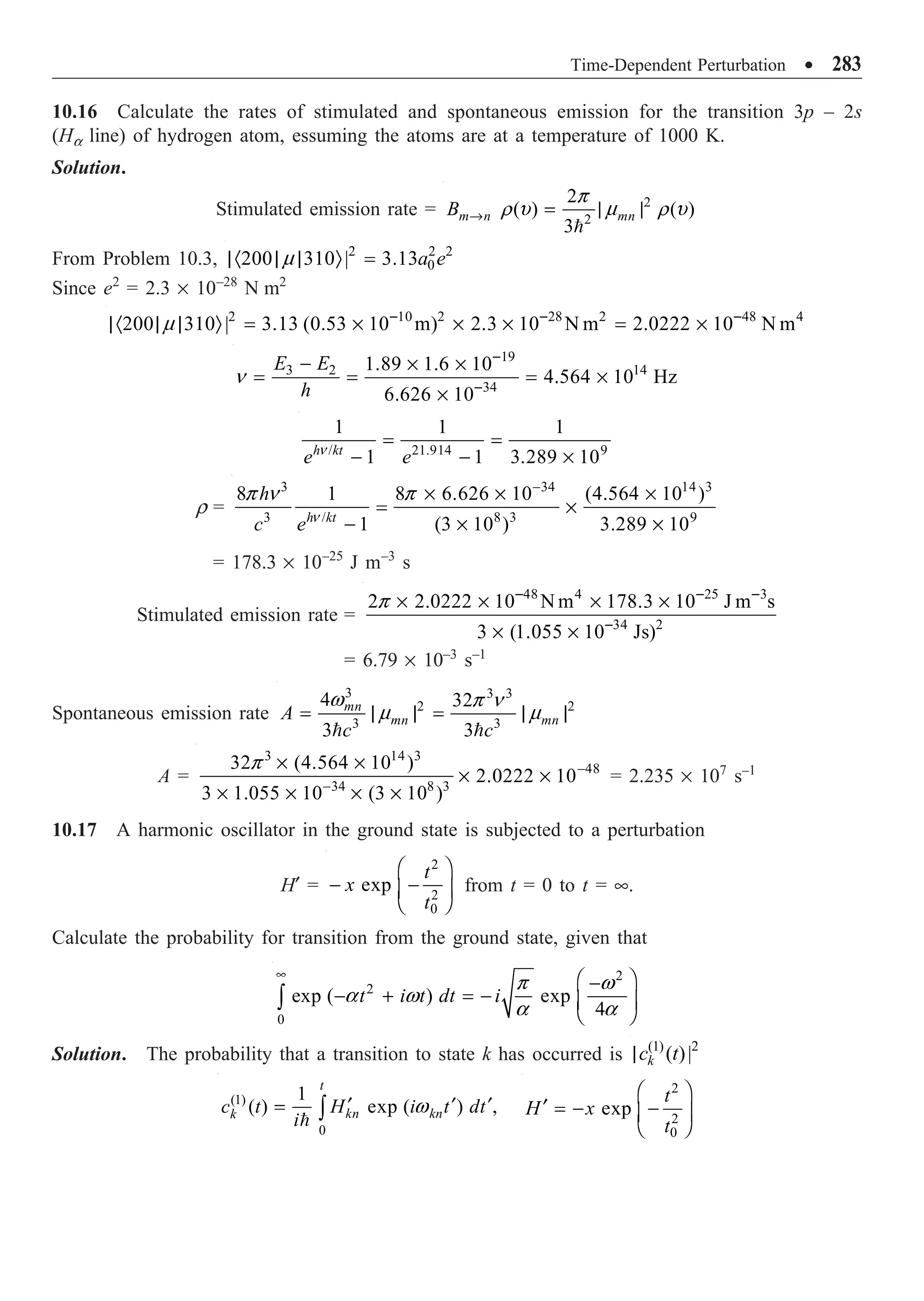
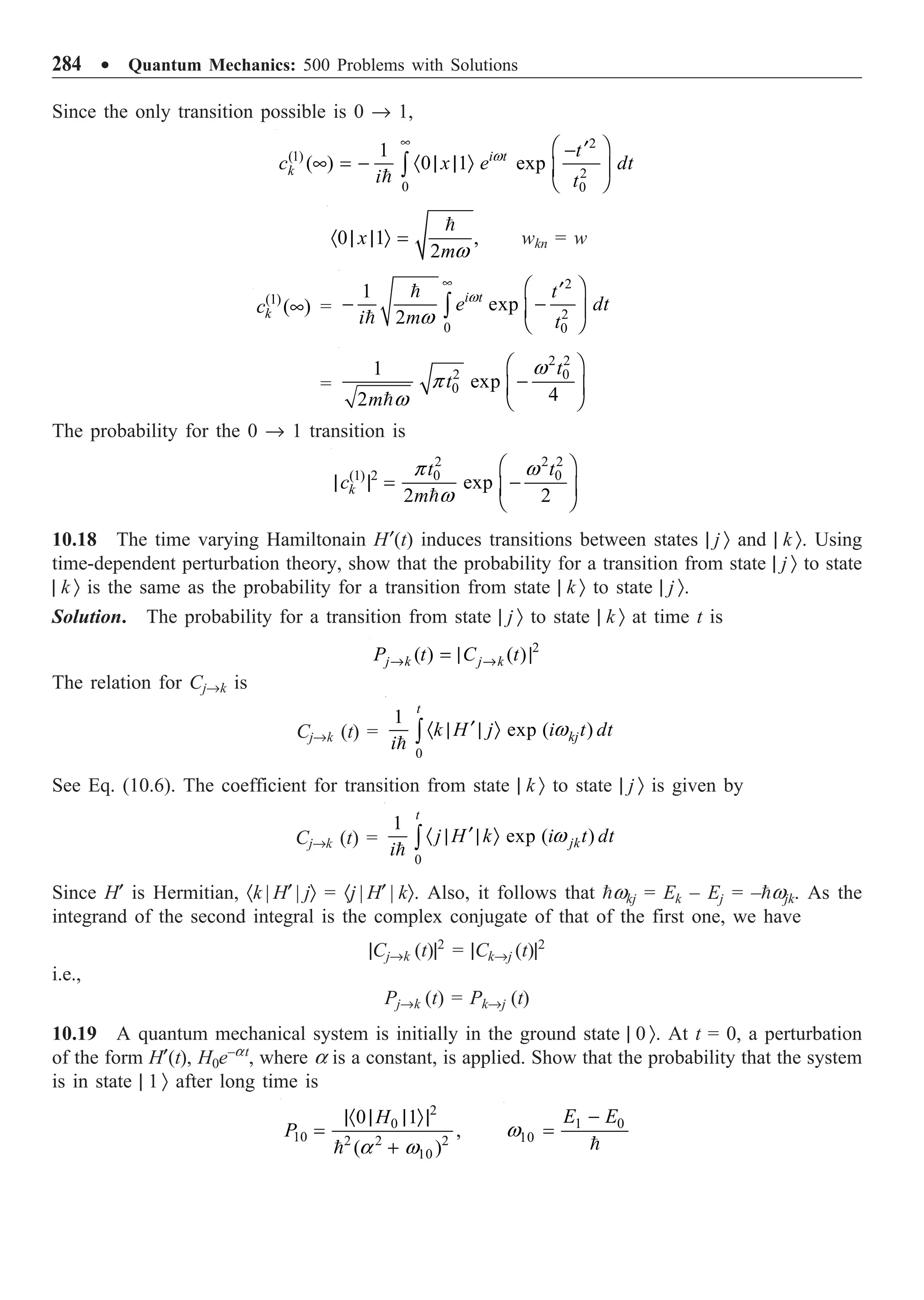
295. Time-Dependent Perturbation ∑ 285
Solution. In the first-order perturbation, the transition probability amplitude is given by Eq. (10.6).
So,
(1)
0
1
( ) exp ( )
t
kn kn
k
C t H i t dt
i
¢ ¢ ¢
= Ú
w
where
kn
H k H n
¢ ¢
= · | | Ò , k n
kn
E E
-
=
w
Substituting the value of H¢ and allowing t Æ •, we get
(1)
( )
k
C t = 10 0
0
1
exp ( ) 1 0
t
i t e H dt
i
•
-
· | | Ò
Ú
a
w
=
0 10
10 0
1 0 exp [ ( ) ]
( )
H i t
i i
a w
a w
•
· | | Ò - -
È ˘
Í ˙
- -
Î ˚
=
0
10
1 0 1
H
i i
a w
· | | Ò
-
The probability for a transition from state | 0 Ò to state | 1 Ò after a long time is
2
(1) 2 0
10 2 2 2 2
10
0 1
| |
( )
k
H
P C
a
|· | | Ò|
=
+
w
10.20 A hydrogen atom in the ground state is subjected to an electric field
E = E0e–t/t
, t 0, t being constant
along the z-axis. Calculate the probability for transition to the (200) and (210) states when it is very
large.
Solution. The interaction Hamiltonian
H¢ = /
0
cos cos
t
E erE e
m -
- ◊ - = t
m q q
E =
y100 = 0
1/2
/
3
0
1 r a
e
a
-
Ê ˆ
Á ˜
Ë ¯
p
y200 = 0
3/2
/
1/2
0 0
1 1
1
2 2
r a
r
e
a a
-
Ê ˆ Ê ˆ
-
Á ˜ Á ˜
Ë ¯ Ë ¯
p
y210 = 0
5/2
/2
1/2
0
1 1
cos
2
r a
r e
a
-
Ê ˆ
Á ˜
Ë ¯
q
p
The probability for transition from n Æ k state is
2
2
0
1
( , ) exp ( )
t
n k kn kn
P H r t i t dt
Æ ¢
= Ú
w k n
kn
E E
-
=
w

296. 286 ∑ Quantum Mechanics: 500 Problems with Solutions
(100) to (200) transition:
/
21 200 0 100
( ) 200 100 ( cos )
t
H t H erE e d
-
¢ ¢
= · | | Ò = Ú
t
y q y t
The q-part of the integral is
0
cos sin 0
d =
Ú
p
q q q
Hence, H¢21 is zero. Therefore, the probability PnÆk = 0.
(100) to (210) transition:
0
2
/
3 /2
4 2
0
21 5/2 4
0 0 0
0
( ) 200 100 cos sin
2
t
r a
eE e
H t H r e dr d d
a
•
-
-
¢ ¢
= · | | Ò = Ú Ú Ú
p p
t
q q q f
p
Writing y = cos q, dy = – sin q dq,
we have
1
2 2
0 1
2
cos sin
3
d y dy
-
= - =
Ú Ú
p
q q q
H¢
21(t) =
/
0
5/2 4 5
0 0
4 ! 2
2
3
2 (3/2 )
t
eE e
a a
-
◊ ¥ ¥
t
p
p
=
/
/
0 0
256
243 2
t
t
eE a e
Ae
-
-
=
¥
t
t
where
A = 0 0
256
243 2
eE a
¥
21 21
/ /
21 21 21
0 0 0
(cos sin )
t t t
i t i t
t t
H e dt A e e dt A e t i t dt
- -
¢ = = +
Ú Ú Ú
w w
t t
w w
As t is very large, we can assume the limits of integral as 0 to •. Then,
21 21
21 2 2 2 2
0 21 21
1/
(1/ ) + (1/ ) +
i t
H e dt A i
• Ê ˆ
¢ = +
Á ˜
Ë ¯
Ú
w w
t
t w t w
P1Æ2 =
2
21 21
2 2 2 2 2 2 2 2 2
21 21 21 21
1/ 1/
(1/ ) + (1/ ) + (1/ ) + (1/ ) +
A
i i
Ê ˆ Ê ˆ
+ -
Á ˜ Á ˜
Ë ¯ Ë ¯
w w
t t
t w t w t w t w
=
2
2 2
21
2 2 2 2 2 2 2
21 21
(1/ )
[(1/ ) + ] [(1/ ) + ]
A
i
Ê ˆ
+
Á ˜
Ë ¯
w
t
t w t w
=
2
2 2 2
21
1
(1/ ) +
A Ê ˆ
Á ˜
Ë ¯
t w

297. 287
Systems of identical particles are of considerable importance for the understanding of structures of
atoms, molecules and nuclei.
11.1 Indistinguishable Particles
Particles that can be substituted for each other with no change in the physical situation are said to
be indistinguishable or identical. For example, n electrons are strictly indistinguishable. Since the
interchange of coordinates of any two electrons does not change the Hamiltonian, we have
H (1, 2, º, i, j, º, n) = H (1, 2, º, i, j, º, n) (11.1)
A particle exchange operator Pij is defined such that when it operates on a state, the coordinates
of particles i and j are interchanged. The eigenvalue of the particle exchange operator is either +1
or –1, i.e.,
Pijy (1, 2, º, i, j, º, n) = ±1y (1, 2, º, j, i, º, n) (11.2)
Consequently, the indistinguishability requires that the wave function must be either symmetric or
antisymmetric with respect to the interchange of any pair of particles. The symmetry character of a
wave function does not change with time.
The solution of the Schrödinger equation of an n-identical particle system gives y which is a
function of the coordinates of the n particles. This leads to n ! solutions from one solution since
n ! permutations of the n arguments are possible. All these n ! solutions correspond to the same
energy. The degeneracy arising due to this interchange is called exchange degeneracy.
11.2 The Pauli Principle
From simple considerations, Pauli has shown that the symmetry of a system is related to the spin of
the identical particles:
Identical Particles
CHAPTER 11

298. 288 ∑ Quantum Mechanics: 500 Problems with Solutions
1. Systems of identical particles with half odd integer spins (spin 1/2, 3/2, 5/2, º) are
described by antisymmetric wave functions. Such particles obey Fermi-Dirac statistics and
are called fermions.
2. Systems of identical particles with integer spins (spin 0, 1, 2, º) are described by
symmetric wave functions. Such particles obey Bose-Einstein statistics and are called
bosons.
One form of Pauli’s exclusion principle is that two identical fermions cannot occupy the same
state. For electrons, this is stated as “No two electrons can have the same set of quantum numbers”.
For a system having n particles, if ua(1), ub(2), º, un(n) are the n1 particle eigenfunctions, the
normalized antisymmetric combination is given by the Slater determinant
as
(1) (2) ( )
(1) (2) ( )
1
(1, 2, 3, , )
!
(1) (2) ( )
a a a
b b b
n n n
u u u n
u u u n
n
n
u u u n
=
…
…
…
…
y (11.3)
The factor 1/ !
n is the normalization constant.
11.3 Inclusion of Spin
The spin can be included in the formalism by taking the single particle eigenfunctions of both
position wave function f (r) and spin function c(ms), i.e.,
y (r, ms) = f (r)c(ms) (11.4)
The spin functions of spin –1/2 system are discussed in problem
Boson states:
s s
s
as as
(spatial) (spin)
(spatial) (spin)
Ï
Ô
= Ì
Ô
Ó
y c
y
y c
(11.5)
Fermion states:
s as
as
as s
(spatial) (spin)
(spatial) (spin)
Ï
Ô
= Ì
Ô
Ó
y c
y
y c
(11.6)
Here, s refers to symmetric and as refers to antisymmetric.
For a system with two identical electrons, the possible spin product functions alongwith the
eigenvalues are given in Table 11.1.
Table 11.1 Two Electron Spin Product Functions
Spin product functions Symmetry character Eigenvalue of Eigenvalue of
Sz = S1z + S2z S2
= (S1 + S2)2
aa Symmetric 22
1
( )
2
+
ab ba Symmetric 0 22
bb Symmetric – 22
1
( )
2
-
ab ba Antisymmetric 0 0

299. Identical Particles ∑ 289
PROBLEMS
11.1 Consider a system having three identical particles. Its wave function y (1,2,3) is 3 ! fold
degenerate due to exchange degeneracy. (i) Form symmetric and antisymmetric combinations of the
degenerate functions. (ii) If the Hamiltonian H(1,2,3) = H(1) + H(2) + H(3) and y (1,2,3) =
ua(1) ub(2) uc(3), where ua(1) ub(2) and uc(3) are the eigenfunctions of H1, H2, H3 respectively, what
are the symmetric and antisymmetric combinations?
Solution.
(i) In the three-particle system the wave function y (1,2,3) = 6-fold degenerate. The six
functions are y (123), y (132), y (321), y (213), y (231), and y (312).
The symmetric combination is the sum of all functions:
ys = y (123) + y (132) + y (321) + y (213) + y (231) + y (312)
The antisymmetric combination is the sum of all functions with even number of interchanges–the
sum of all functions with odd number of interchanges.
yas = y (123) + y (231) + y (312) – y (213) + y (132) + y (321)
(ii) y (1,2,3) = ua(1) ub(2) uc(3)
The six product functions are
ua(1) ub(2) uc(3), ua(1) ub(3) uc(2), ua(2) ub(1) uc(3)
ua(2) ub(3) uc(1), ua(3) ub(2) uc(1), ua(3) ub(1) uc(2)
The symmetric combination of these is simply the sum. The antisymmetric combination
yas = ua(1) ub(2) uc(3) + ua(2) ub(3) uc(1) + ua(3) ub(1) uc(2)
– ua(1) ub(3) uc(2) – ua(2) ub(1) uc(3) – ua(3) ub(2) uc(1)
=
(1) (2) (3)
1
(1) (2) (3)
3 !
(1) (2) (3)
a a a
b b b
c c c
u u u
u u u
u u u
;
1
3 !
is the normalization constant
11.2 Consider a one-dimensional infinite square well of width 1 cm with free electrons in it. If its
Fermi energy is 2 eV, what is the number of electrons inside the well?
Solution. In an infinite square well, energy
2 2 2
2
,
2
n
n
E
ma
=
p
n = 1, 2, 3, º
Each level accommodates two electrons, one spin up and the other spin down. If the highest filled
level is n, then the Fermi energy EF = En.
n2
=
2
F
2 2
2
E ma
p
=
19 31 2
2 34 2
(2 1.6 10 J) 2 (9.1 10 kg)(0.01 m)
(1.05 10 J s)
p
- -
-
¥ ¥ ¥ ¥ ¥
¥
= 5.3475 ¥ 104
n = 2.312 ¥ 107
The number of electrons inside the well = 2n = 4.62 ¥ 107
.

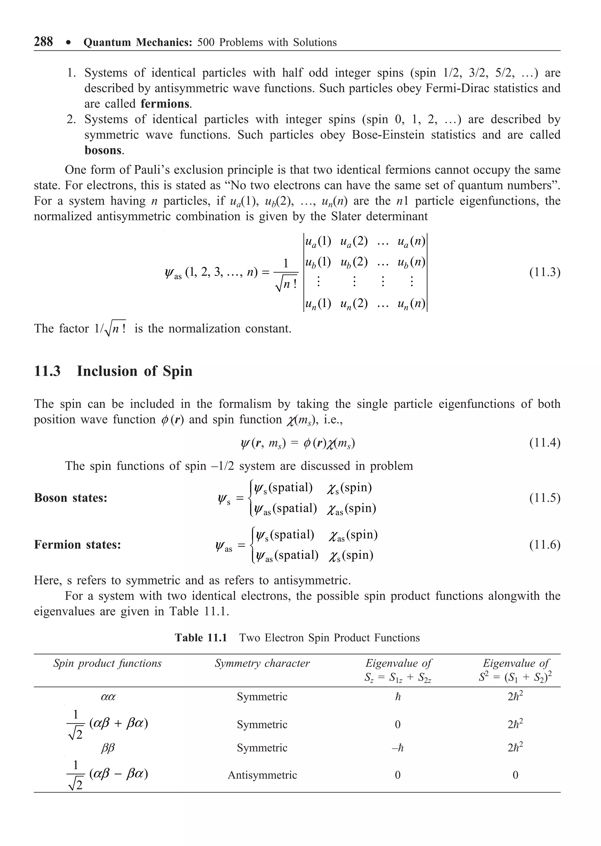
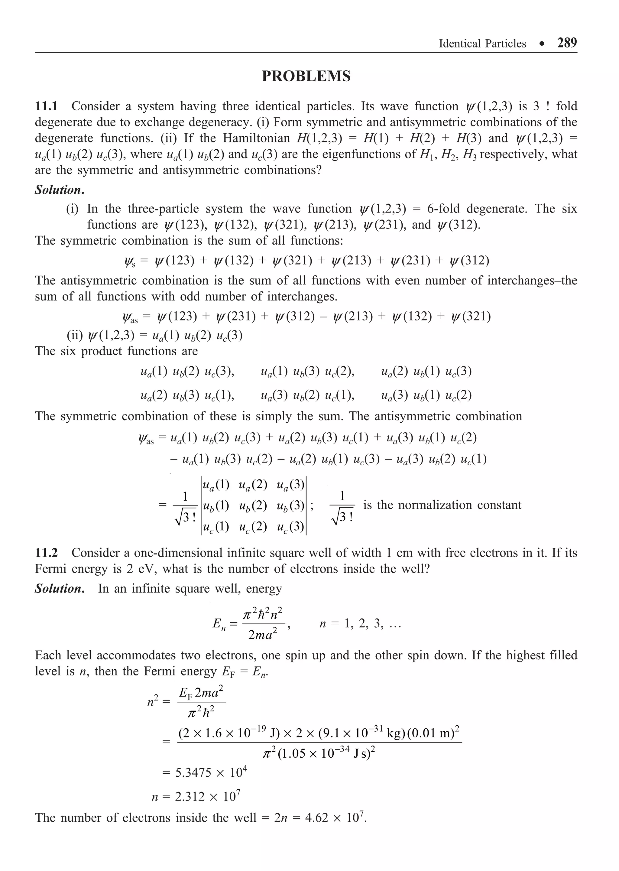
300. 290 ∑ Quantum Mechanics: 500 Problems with Solutions
11.3 N noninteracting bosons are in an infinite potential well defined by V(x) = 0 for 0 x a;
V (x) = • for x 0 and for x a. Find the ground state energy of the system. What would be the
ground state energy if the particles are fermions.
Solution. The energy eigenvalue of a particle in the infinite square well (Problem 4.1) is given by
En =
2 2 2
2
,
2
n
ma
p
n = 1, 2, 3, º
As the particles are bosons, all the N particles will be in the n = 1 state. Hence the total energy
E =
2 2
2
2
N
ma
p
If the particles are fermions, a state can have only two of them, one spin up and the other spin down.
Therefore, the lowest N/2 states will be filled. The total ground state energy will be
E =
2 2
2
2
2ma
p
[12
+ 22
+ 33
+ º + (N/2)2
]
=
2 2
2
1
1 2 1
6 2 2 2
N N N
ma
È ˘
Ê ˆ Ê ˆ
+ +
Í ˙
Á ˜ Á ˜
Ë ¯ Ë ¯
Î ˚
p
=
2 2
2
24ma
p
N (N + 1) (N + 2)
11.4 Consider two noninteracting electrons described by the Hamiltonian
H =
2 2
1 2
2 2
p p
m m
+ + V(x1) + V(x2)
where V(x) = 0 for 0 x a; V(x) = • for x 0 and for x a. If both the electrons are in the same
spin state, what is the lowest energy and eigenfunction of the two-electron system?
Solution. As the electrons are noninteracting, the wave function of the system y (1, 2) can be
written as
y (1, 2) = y (1) y (2)
With this wave function, the Schrödinger equation for the system breaks into two one-particle
equations:
2 2
2
1
(1)
2
d
m dx
-
y + V(x1) y (1) = E(1)
y (1)
2 2
2
2
(2)
2
d
m dx
-
y + V(x2) y (1) = E(2)
y (1)
where E(1)
+ E(2)
= E, which is the total energy of the system. The energy eigenvalues and
eigenfunctions for a single particle in such a potential (see Problem 4.1) are

301. Identical Particles ∑ 291
1
2 2 2
(1) 1
2
,
2
n
n
E
ma
=
p
1
1 1
2
(1) sin ,
n
n x
a a
=
p
y n1 = 1, 2, 3, º
2
2 2 2
(1) 2
2
,
2
n
n
E
ma
=
p
2
2 2
2
(2) sin ,
n
n x
a a
=
p
y n2 = 1, 2, 3, ....
As both the electrons are in the same spin state, the possible combinations of spin functions are a (1)
a (2) or b (1) b (2), both being symmetric. Hence the space function must be antisymmetric. As the
electrons are either spin up (aa) or spin down (bb), n1 = n2 = 1 is not possible. The next possibility
is n1 = 1, n2 = 2.
Energy of the state (n1 = 1, n2 = 2) =
2 2 2 2 2 2
2 2 2
4 5
2 2 2
ma ma ma
+ =
p p p
Energy eigenfunction y (1, 2) = 1 2
2
2
sin sin
x x
a a a
p p
When the two electrons are interchanged, the eigenfunction
y (2, 1) = 2 1
2
2
sin sin
x x
a a a
p p
Since both the states have the same energy, the space wave function of the system must be a linear
combination of the two functions. The antisymmetric combination is
y (1, 2) – y (2, 1)
To get the complete energy eigenfunction, this space part has to be multiplied by aa or bb. Since
the energy depends only on the space part,
Energy eigenvalue E =
2 2
2
5
2ma
p
11.5 Show that for a system of two identical particles of spin I, the ratio of the number of states
which are symmetric under spin interchange to the number of states which are antisymmetric under
spin interchange is (I + 1)/I.
Solution. We shall denote the mI values of the two spins by mI and m¢I. The spin states of the
combined system are given by | mI (1)Ò | m¢I (2)Ò. The products | mI (1)Ò | mI (2)Ò corresponding to
mI = m¢I will be symmetric and we will have (2I + 1) such product functions. The number of product
functions corresponding to mI π m¢I will be 2I (2I + 1). With these we have to form combinations
of the type
| mI (1)Ò | m¢I (2)Ò ± | m¢I (1)Ò | mI (2)Ò
where the plus sign gives symmetric and the minus sign gives antisymmetric functions. As we take
two product functions to form such a combination, we will have (1/2) 2I (2I + 1) symmetric and
(1/2) 2I (2I + 1) antisymmetric combinations. The total number of symmetric combinations =
(2I + 1) + (1/2) 2I (2I + 1) = (I + 1) (2I + 1). Hence,
No. of symmetric combinations ( 1) (2 1) 1
No. of antisymmetric combinations (2 1)
I I I
I I I
+ + +
= =
+

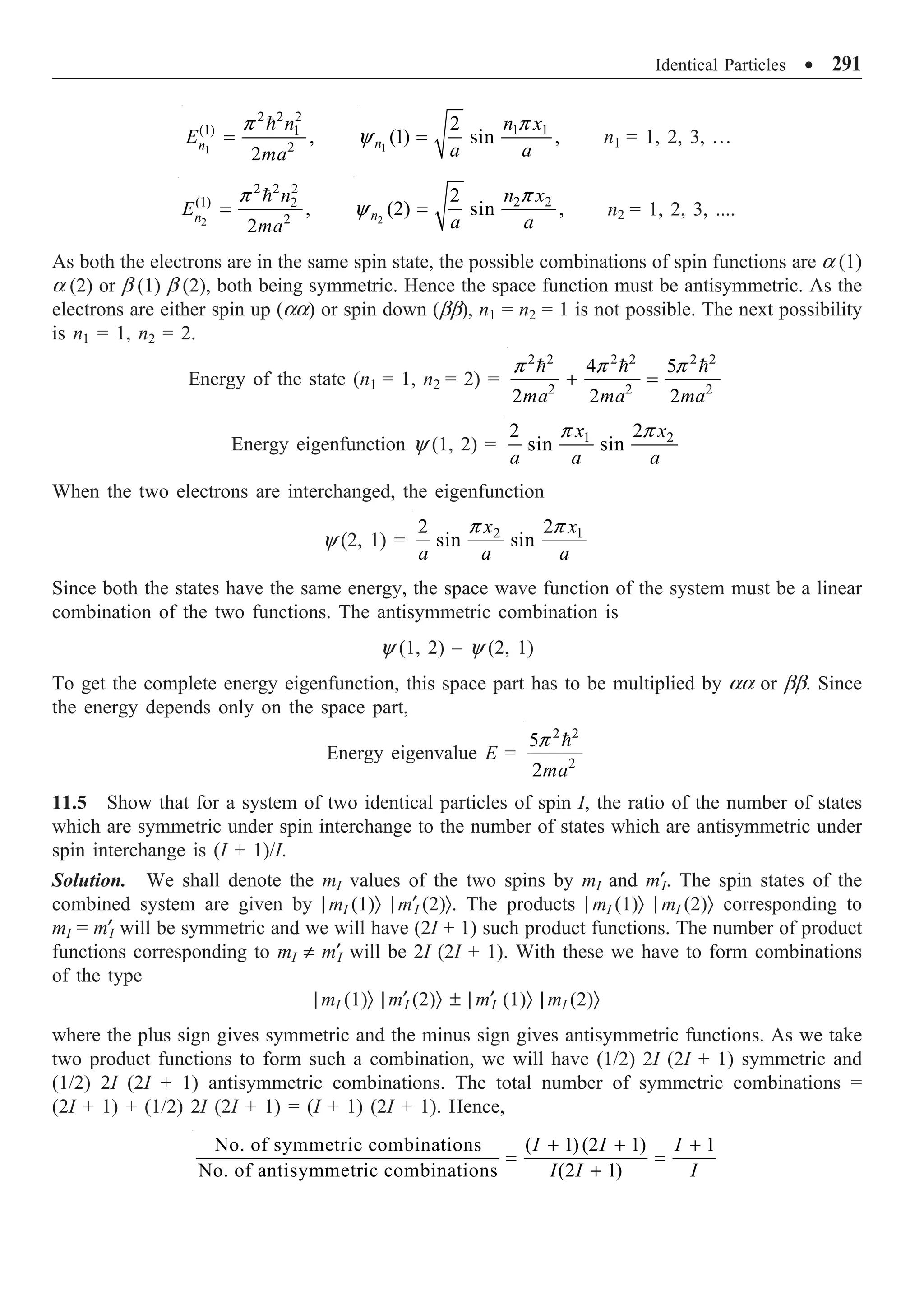
302. 292 ∑ Quantum Mechanics: 500 Problems with Solutions
11.6 Show that if a wave function y (1, 2, 3, º, n) is an energy eigenfunction of a symmetric
Hamiltonian that corresponds to a nondegenerate eigenvalue, it is either symmetric or antisymmetric.
Solution. The eigenvalue equation of the Hamiltonian is
H(1, 2, º, i, j, º, n) y (1, 2, º, i, j, º, n) = Ey (1, 2, º, i, j, º, n)
Interchange of the indistinguishable particles i and j does not change the energy. Hence,
H(1, 2, º, j, i, º, n) y (1, 2, º, j, i, º, n) = Ey (1, 2, º, j, i, º, n)
Since H is symmetric,
H(1, 2, º, i, j, º, n) y (1, 2, º, j, i, º, n) = Ey (1, 2, º, j, i, º, n)
H(1, 2, º, i, j, º, n) Pijy (1, 2, º, i, j, º, n) = EPijy (1, 2, º, i, j, º, n)
= PijH (1, 2, º, i, j, º, n) y (1, 2, º, i, j, º, n)
(HPij – PijH) y = 0 or [H, Pij] = 0
Since Pij commutes with the Hamiltonian, y (1, 2, º, i, j, º, n) is an eigenfunction of Pij also.
Pijy (1, 2, º, i, j, º, n) = py (1, 2, º, i, j, º, n)
y (1, 2, º, j, i, º, n) = py (1, 2, º, i, j, º, n)
Operating both sides by Pij, we get
y (1, 2, º, i, j, º, n) = p2
y (1, 2, º, i, j, º, n)
Hence, p2
= 1 or p = ±1, i.e.,
Pijy (1, 2, º, i, j, º, n) = ±y (1, 2, º, i, j, º, n)
which means that the wavefunction must be either symmetric or antisymmetric with respect to
interchange of two identical particles.
11.7 Sixteen noninteracting electrons are confined in a potential V(x) = • for x 0 and x 0;
V(x) = 0, for 0 x a.
(i) What is the energy of the least energetic electron in the ground state?
(ii) What is the energy of the most energetic electron in the ground state?
(iii) What is the Fermi energy Ef of the system?
Solution.
(i) The least energetic electron in the ground state is given by
2 2
1 2
.
2
E
ma
=
p
(ii) In the given potential, the energy eigenvalue
2 2 2
2
,
2
n
n
E
ma
=
p
n = 1, 2, 3, º
As two electrons can go into each of the states n = 1, 2, 3, º, the highest filled level will
have n = 8 and its energy will be
2 2 2 2 2
8 2 2
8 32
2
E
ma ma
= =
p p

303. Identical Particles ∑ 293
(iii) The energy of the highest filled state is the Fermi energy EF. Hence,
2 2
2
32
F
E
ma
=
p
11.8 What is the ground state energy and wave function for two identical particles in the potential
defined in Problem 11.7 if the two particles are (i) bosons, and (ii) fermions?
Solution. The solution of the Schrödinger equation of a particle in the given potential gives
2 2 2
2
,
2
n
n
E
ma
=
p 2
( ) sin ,
n
n x
x
a a
=
p
y n = 1, 2, 3, º
(i) Bosons: Both the particles can be in the same state. Hence,
2 2
1 2
(1) ,
2
E
ma
=
p 1
1 1
2
( ) sin
x
x
a a
=
p
y
2 2
1 2
(2) ,
2
E
ma
=
p 2
2 2
2
( ) sin
x
x
a a
=
p
y
The energy and wave function of the combined system are
2 2
1 1 2
(1) (2) ,
E E E
ma
= + =
p 1 2
2
sin sin
x x
a a a
Ê ˆ
= Á ˜
Ë ¯
p p
y
Interchange does not change y. Hence it is symmetric. Therefore, the spin function of the two-
particle system must be symmetric. The wave function of the system including spin is
1 2
2
( , ) sin sin
( )/ 2
s
x x
x m
a a a
Ï
Ô
Ê ˆ Ô
= Ì
Á ˜
Ë ¯ Ô
+
Ô
Ó
aa
p p
y bb
ab ba
(ii) Fermions: In the ground state, one particle has to be spin up and the other spin down.
Hence the energy and wave functions are
2 2
2
,
E
ma
=
p 1 2
2 1
( , ) sin sin ( )
2
s
x x
x m
a a a
Ê ˆ
= -
Á ˜
Ë ¯
p p
y ab ba
11.9 Consider two identical particles described by the Hamiltonian
2 2
2 2 2 2
1 1 2 2
1 2
( ) ( ) 1 1
2 2 2 2
p x p x
H m x m x
m m
= + + +
w w
Obtain the energy spectrum of this system. Discuss its degeneracy.
Solution. The Schrödinger equation of the system splits into two equations:
2 2
2 2
1 1 1 1
2
1
1
( ) ( )
2 2
d
m x x E x
m dx
Ê ˆ
- + =
Á ˜
Ë ¯
w y y

304. 294 ∑ Quantum Mechanics: 500 Problems with Solutions
2 2
2 2
2 2 2 2
2
2
1
( ) ( )
2 2
d
m x x E x
m dx
Ê ˆ
- + =
Á ˜
Ë ¯
w y y
The solution of these equations is
1 1
1
;
2
n
E n
Ê ˆ
= +
Á ˜
Ë ¯
w
2
1
1
/2
1 1
( ) ( ) ,
y
n n
x NH y e-
=
y
1/2
1 1
m
y x
Ê ˆ
= Á ˜
Ë ¯
w
2 2
1
;
2
n
E n
Ê ˆ
= +
Á ˜
Ë ¯
w
2
2
2
/2
2 2
( ) ( ) ,
y
n n
x NH y e-
=
y
1/2
2 2
m
y x
Ê ˆ
= Á ˜
Ë ¯
w
where n1 = 0, 1, 2, º; n2 = 0, 1, 2, 3, º
Total energy 1 2 1 2
( ) ( 1)
n n n
E E E n n n
= + = + + = +
w w w
Wave function of the system yn (x1, x2) = 1 1 2 2
( ) ( )
n n
x x
y y
Each level is (n + 1)-fold degenerate.
11.10 Prove that the three column vectors
1 0 0
0 , 1 , 0
0 0 1
Ê ˆ Ê ˆ Ê ˆ
Á ˜ Á ˜ Á ˜
Á ˜ Á ˜ Á ˜
Á ˜ Á ˜ Á ˜
Ë ¯ Ë ¯ Ë ¯
are the spin eigenfunctions of Sz of a spin s = 1 system. Also prove that they are mutually orthogonal.
Solution. The Sz matrix of a spin s = 1 system is given by
Sz =
1 0 0
0 0 0
0 0 1
Ê ˆ
Á ˜
Á ˜
Á ˜
-
Ë ¯
1 0 0 1 1 1
0 0 0 0 0 1 0
0 0 1 0 0 0
Ê ˆ Ê ˆ Ê ˆ Ê ˆ
Á ˜ Á ˜ Á ˜ Á ˜
= =
Á ˜ Á ˜ Á ˜ Á ˜
Á ˜ Á ˜ Á ˜ Á ˜
-
Ë ¯ Ë ¯ Ë ¯ Ë ¯
1 0 0 0 0 0
0 0 0 1 0 0 1
0 0 1 0 0 0
Ê ˆ Ê ˆ Ê ˆ Ê ˆ
Á ˜ Á ˜ Á ˜ Á ˜
= =
Á ˜ Á ˜ Á ˜ Á ˜
Á ˜ Á ˜ Á ˜ Á ˜
-
Ë ¯ Ë ¯ Ë ¯ Ë ¯
1 0 0 0 0 0
0 0 0 0 0 1 0
0 0 1 1 1 1
Ê ˆ Ê ˆ Ê ˆ Ê ˆ
Á ˜ Á ˜ Á ˜ Á ˜
= = -
Á ˜ Á ˜ Á ˜ Á ˜
Á ˜ Á ˜ Á ˜ Á ˜
- -
Ë ¯ Ë ¯ Ë ¯ Ë ¯

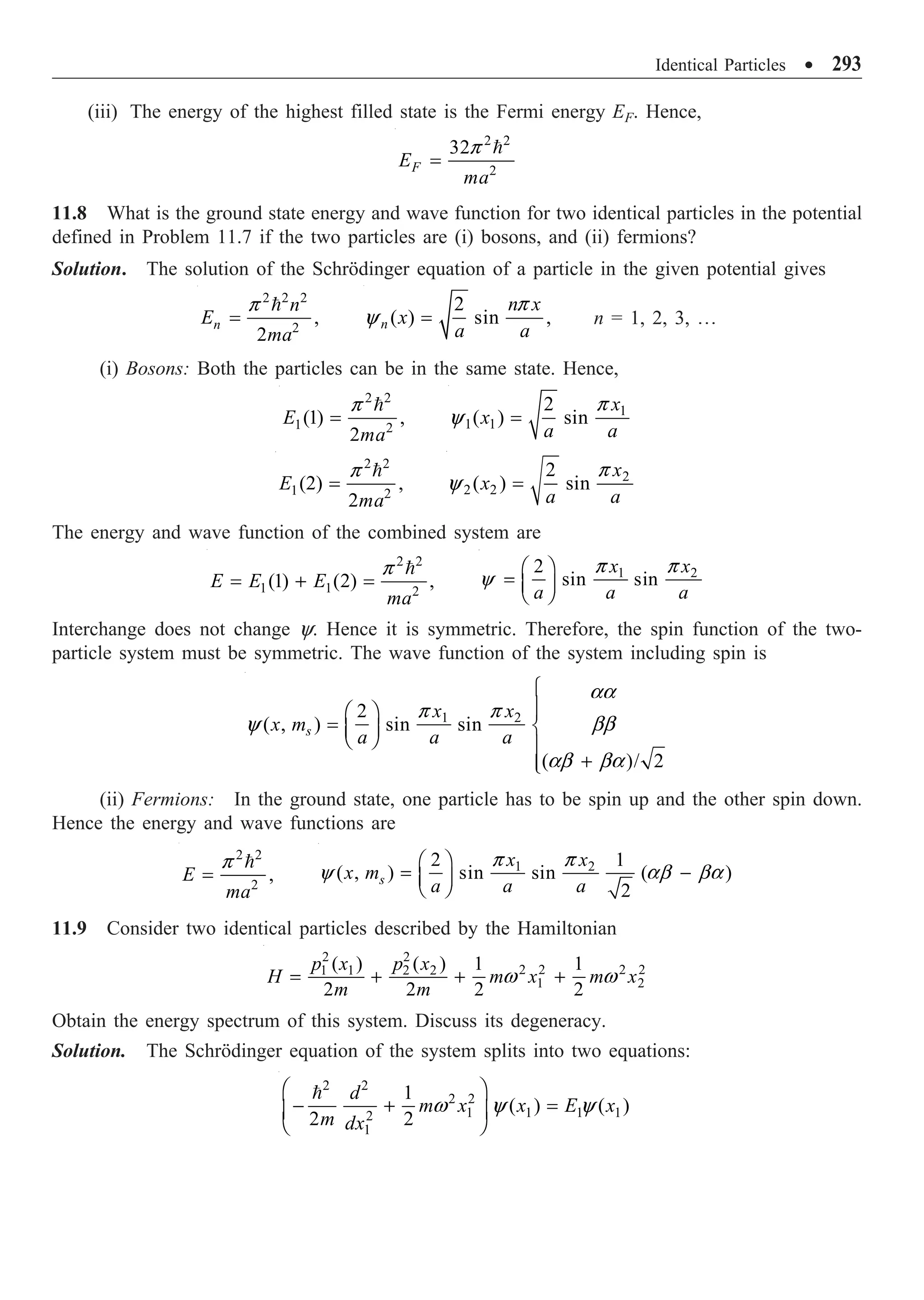
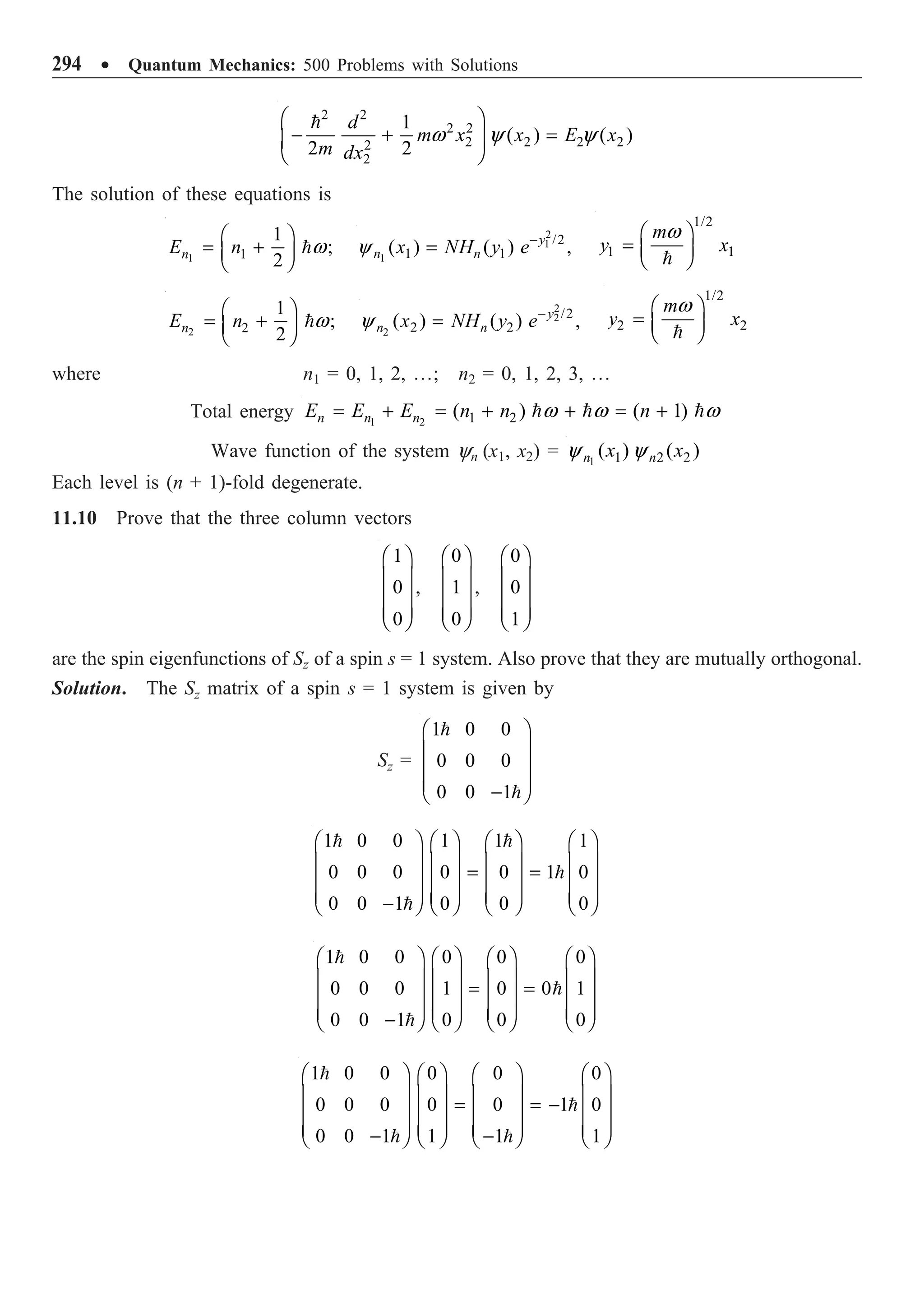
305. Identical Particles ∑ 295
As expected, the eigenvalues of Sz are 1, 0 and –1. Thus,
0
(1 0 0) 1 0,
0
Ê ˆ
Á ˜ =
Á ˜
Á ˜
Ë ¯
0
(0 1 0) 0 0,
1
Ê ˆ
Á ˜ =
Á ˜
Á ˜
Ë ¯
1
(0 0 1) 0 0
0
Ê ˆ
Á ˜ =
Á ˜
Á ˜
Ë ¯
Hence the result.
11.11 Give the zeroth order wave functions for helium atom (i) in the ground state (1s2
), and
(ii) in the excited state 1s 2s. Also, express them in the form of Slater determinants.
Solution.
(i) The ground state of helium is 1s2
. As both the electrons are in the y100 state, the space part
of the wave function is y100(r1)y100(r2). The spin part that multiplies this must be antisymmetric so
that the total wave function is antisymmetric. Hence, the zeroth order wave function for helium atom
in the 1s2
state is
1s(1) 1s (2)
1
[ (1) (2) (1) (2)]
2
-
a b b a
In terms of the Slater determinant, this takes the form
1s(1) (1) 1s(2) (2)
1
1s(1) (1) 1s(2) (2)
2
a a
b b
(ii) For the 1s 2s state, taking exchange degeneracy into account, the possible product
functions are
1s(1)2s(2) and 1s(2) 2s(1)
The symmetric combination ys and the antisymmetric combination yas are given by
ys =
1
2
[1s(1) 2s(2) + 1s(2) 2s(1)]
yas =
1
2
[1s(1) 2s(2) – 1s(2) 2s(1)]
Combining these with the spin wave function for a two-electron system, with the condition that the
total wave function must be antisymmetric, we get
y1 =
1
2
[1s(1) 2s(2) + 1s(2) 2s(1)] [a (1) b (2) – b (1) a (2)]
1
2
y2 =
1
2
[1s(1) 2s(2) – 1s(2) 2s(1)] a (1) a (2)
y3 =
1
2
[1s(1) 2s(2) – 1s(2) 2s(1)] [a (1) b (2) + b (1) a (2)]
1
2
y4 =
1
2
[1s(1) 2s(2) – 1s(2) 2s(1)] b (1) b (2)

306. 296 ∑ Quantum Mechanics: 500 Problems with Solutions
For 1s 2s configuration, we have the following spin orbital combinations: 1sa, 1sb, 2sa and 2sb,
leading to the four Slater determinants (the normalization factor 1/ 2 not included.):
D1 =
1s(1) (1) 1s(2) (2)
,
2s(1) (1) 2s(2) (2)
a a
a a
D2 =
1s(1) (1) 1s(2) (2)
2s(1) (1) 2s(2) (2)
a a
b b
D3 =
1s(1) (1) 1s(2) (2)
,
2s(1) (1) 2s(2) (2)
b b
a a
D4 =
1s(1) (1) 1s(2) (2)
2s(1) (1) 2s(2) (2)
b b
b b
A comparison of the above wave functions with these determinants shows that y1, y2, y3, y4 are
equal to the determinants (D2 – D3)/2, D1/ 2 , (D2 + D3)/2 and D4/ 2 , respectively.
11.12 Prove that it is impossible to construct a completely antisymmetric spin function for three
electrons.
Solution. Let a, b, c stand for three functions and 1, 2, 3 for three identical particles. In the function
a(1) b (2) c (3), particle 1 is in a, particle 2 is in b, and particle 3 is in c. Let us proceed without
specifying that these functions correspond to space or spin functions. The third-order Slater
determinant for the case is
(1) (2) (3)
1
(1) (2) (3)
6
(1) (2) (3)
a a a
b b b
c c c
This is completely antisymmetrized as interchange of two spins amounts to interchanging two
columns of the determinant, which multiplies it by –1. Let us now specify the functions a, b, c as
that due to electron spins. Let a = a, b = b and c = b in the above determinant. The determinant
reduces to
(1) (2) (3)
1
(1) (2) (3)
6
(1) (2) (3)
g
a a
b b b
b b b
As the second and third rows of the determinant are identical, its value is zero. In whatever way we
select a, b, c, the two rows of the determinant will be equal. Therefore, we cannot construct a
completely antisymmetric three-electron spin function.
11.13 Two particles of mass m are in a three-dimensional box of sides a, b, c (a b c). The
potential representing the interaction between the particles is V = Ad (r1 – r2), where d is the Dirac
delta function. Using the first-order perturbation theory, calculate the lowest possible energy of the
system if it is equal to (i) spin zero identical particles, (ii) spin half identical particles with spins
parallel. Given
4
0
3
sin
8
a
x
dx a
a
=
Ú
p
.
Solution. The energy eigenvalues and eigenfunctions of a particle in a rectangular box of side a,
b, c are given by (Problem 5.1)
2 2
2
2 2
2 2 2
2
y z
x
n n
n
E
m a b c
Ê ˆ
= + +
Á ˜
Ë ¯
p
, nx, ny, nz = 1, 2, 3, º

307. Identical Particles ∑ 297
8
( , , ) sin sin sin
y z
x
n y n z
n x
x y z
abc a b c
=
p p
p
y
(i) For a system of spin zero particles, the total wave function must be symmetric for
interchange of any pair of particles. Hence, for the two-particle system, the unperturbed wave
function can be taken as the product of two single-particle wave function which is symmetric, i.e.,
ys (r1, r2) = y (r1) y (r2)
= 1 1 1 2 2 2
8
sin sin sin sin sin sin
x y z x y z
abc a b c a b c
p p p p p p
The unperturbed energy
2 2
0 2 2 2
1 1 1
E
m a b c
Ê ˆ
= + +
Á ˜
Ë ¯
p
The Hamiltonian representing the interaction between the two particles is
H¢ = Ad (r1 – r2)
where A is a constant, can be taken as the perturbation. The first order correction to the energy
(1)
s
E = 1 2 1 2 1 2 1 2
*( , ) ( ) ( , )
s s
A d d
-
Ú y d y t t
r r r r r r
=
2
1 1 1
( , )
s
A d
Ú y t
r r
=
4
2
1 1 1
1 1 1
0 0 0
8
sin sin sin
a b c
x y z
A dx dy dz
abc a b c
Ê ˆ
Ê ˆ
Á ˜ Á ˜
Ë ¯ Ë ¯
Ú Ú Ú
p p p
=
2
4 4 4
1 1 1
1 1 1
0 0 0
8
sin sin sin
a b c
x y z
A dx dy dz
abc a b c
Ê ˆ
Á ˜
Ë ¯ Ú Ú Ú
p p p
=
2
8 3 3 3 27
8 8 8 8
a b c A
A
abc abc
Ê ˆ
Á ˜
Ë ¯
Consequently, the energy corrected to first order is
2 2
2 2 2
1 1 1 27
8
s
A
E
m abc
a b c
Ê ˆ
= + + +
Á ˜
Ë ¯
p
(ii) For a system of spin half particles, the total wave function must be antisymmetric for
interchange of any pair of particles. As the spins are parallel, the spin wave function is symmetric
and, therefore, the space part must be antisymmetric. One of the particles will be in the ground state
y111, and the other will be in the first excited state y211 since 1/a2
1/b2
1/c2
. The antisymmetric
combination is then given by
1 2 111 1 211 2 111 2 211 1
1
( , ) [ ( ) ( ) ( ) ( )]
2
a = -
y y y y y
r r r r r r

308. 298 ∑ Quantum Mechanics: 500 Problems with Solutions
The unperturbed energy
Ea =
2 2
2 2 2 2 2 2
1 1 1 4 1 1
2m a b c a b c
Ê ˆ
+ + + + +
Á ˜
Ë ¯
p
=
2 2 2 2
2 2 2 2 2 2
5 2 2 5 1 1
2 2
m m
a b c a b c
Ê ˆ Ê ˆ
+ + = + +
Á ˜ Á ˜
Ë ¯ Ë ¯
p p
The first-order correction to the energy is
(1)
1 2 1 2 1 2 1 2
*( , ) ( ) ( , )
a a a
E A d d
= -
Ú y d y t t
r r r r r r
which reduces to zero when *
a
y and ya are substituted. Hence,
2 2
2 2 2
5 1 1
2
a
E
m a b c
Ê ˆ
= + +
Á ˜
Ë ¯
p
11.14 A one-dimensional infinite potential well of width a contains two spinless particles, each of
mass m. The potential representing the interaction between the particles V = ad (x1 – x2). Calculate
the ground state energy of the system corrected to first order in A.
Solution. The energy eigenvalues and eigenfunctions of a particle in an infinite square well of
width a are given by
En =
2 2 2
2
,
2
n
ma
p
n = 1, 2, 3, º
yn(x) =
2
sin
n x
a a
p
For the two-particle system, the unperturbed wave function
ynk (x1, x2) = 1 2
1 2
2
( ) ( ) sin sin
n k
n x k x
x x
a a a
=
p p
y y
2 2
2 2
2
( ),
2
nk
E n k
ma
= +
p
n, k = 1, 2, 3, º
For the ground state, n = k = 1. The unperturbed ground state energy is, then,
2 2
11 2
E
ma
=
p
Next we consider the perturbation H¢ = Ad(x1 – x2). The first-order correction to the ground state
energy
E(1)
=
2
2 2
1 2
1 2 1 2
0 0
2
sin sin ( )
a a
x x
A x x dx dx
a a a
Ê ˆ
-
Á ˜
Ë ¯ Ú Ú
p p
d
=
4 1
1
2
0
4 3
sin
2
a
x A
A dx
a a
a
=
Ú
p

309. Identical Particles ∑ 299
Hence, the first-order corrected ground state energy
2 2
11 2
3
2
A
E
a
ma
= +
p
11.15 Two identical bosons, each of mass m, move in the one-dimensional harmonic potential
V = (1/2) mw2
x2
. They also interact with each other via the potential
2
int 1 2
exp [ ( ) ]
V a x x
= - -
b
where a and b are positive parameters. Compute the ground state energy of the system to first order
in the parameter a.
Solution. Since the particles are bosons, both of them can remain in the ground state. The Vint term
can be treated as a perturbation. The ground state wavefunction of a harmonic oscillator is
1/4 2
exp
2
m m x
Ê ˆ
Ê ˆ
-
Á ˜ Á ˜
Ë ¯ Ë ¯
w w
p
Hence the unperturbed wavefunction of the ground state for this two-particle system is
y0 (x1, x2) =
1/4 1/4
2 2
1 2
exp exp
2 2
m x m x
m m
Ê ˆ Ê ˆ
Ê ˆ Ê ˆ
- -
Á ˜ Á ˜
Á ˜ Á ˜
Ë ¯ Ë ¯
Ë ¯ Ë ¯
w w
w w
p p
=
1/4
2 2
1 2
exp ( )
2
m m
x x
Ê ˆ È ˘
- +
Á ˜ Í ˙
Ë ¯ Î ˚
w w
p
The first-order correction to the energy
E(1)
=
2 2 2 2 2
1 2 1 2 1 2
exp ( ) ( )
m m
x x x x dx dx
•
-•
È ˘
- + - +
Í ˙
Î ˚
Ú Ú
wa w
b
p
=
1
( / ) 2
m
m +
wa
p w b
The ground state energy of the system is, therefore,
1
( / ) 2
m
E
m
= +
+
wa
w
p w b
11.16 Consider the rotation of the hydrogen molecule H2. How does the identity of the two nuclei
affect the rotational spectrum? Discuss the type of transition that occurs between the rotational levels.
Solution. The rotational energy levels of hydrogen molecule are given by
2
( 1)
,
2
l l
E
I
+
=
l = 0, 1, 2, º
The total wave function of the molecule y is the product of electronic (ye), vibrational (yv),
rotational (yr) and nuclear (yn) wave functions.
y = yeyvyryn

310. 300 ∑ Quantum Mechanics: 500 Problems with Solutions
The spin of proton is half . Hence the total wave function y must be antisymmetric to nuclear
exchange. Since ye and yv are symmetric to nuclear exchange, the product yryn must be
antisymmetric. For l = 0, 2, 4, º, the rotational wave function yr is symmetric with respect to
nuclear exchange and for l = 1, 3, 5, º, it is antisymmetric. Hence, the antisymmetric yn combines
with yr of even l states and the symmetric yn combines with yr of odd l states. As there is no
interconversion between symmetric and antisymmetric nuclear spin states, transitions can take place
between odd l and even l values. Since three symmetric nuclear spin functions and one anitsymmetric
functions are possible (similar to electron product functions), the transitions between odd l values are
considered to be strong. In other words, there will be an alternation in intensity of the rotational
spectrum of H2 molecule.
Note: The hydrogen molecules corresponding to antisymmetric nuclear spin states are called para-
hydrogen, and those corresponding to symmetric spin states are called ortho-hydrogen.
11.17 Obtain the zeroth-order wave function for the state 1s2
2s of lithium atom.
Solution. The 1s orbital accomodates two electrons with opposite spins and 2s orbital the third
electron. The third-order Slater determinant is given by
(1) (2) (3)
1
(1) (2) (3)
6
(1) (2) (3)
a a a
b b b
c c c
where a, b, c stands for the three functions and 1, 2, 3 for the three identical particles. Identifying
a, b, c with the spin-orbitals: a(1) = 1s(1) a (1), b(1) = 1s(1) b (1), c(1) = 2s(1) a (1), the above
determinant becomes
1 (1) (1) 1 (2) (2) 1 (3) (3)
1
1 (1) (1) 1 (2) (2) 1 (3) (3)
6
2 (1) (1) 2 (2) (2) 2 (3) (3)
s a s s
s s s b
s s s
a a
b b
a a a
An equally good ground state is when we take c(1) = 2s(1) b(1).
11.18 Consider a system of two identical particles occupying any of three energy levels A, B and
C having energies E, 2E and 3E, respectively. The level A is doubly degenerate (A1 and A2) and the
system is in thermal equilibrium. Find the possible configurations and the corresponding energy in
the following cases:
(i) the particles obey Fermi statistics;
(ii) the particles obey Bose statistics; and
(iii) the particles are distinguishable and obey Boltzmann statistics.
Solution. Denote the two states with energy E by A1 and A2 and the states with 2E and 3E by B
and C, respectively.
If particle 1 is in A1 and particle 2 is in A2, the configuration is marked as (A1, A2). Thus, the
symbol (B, C) indicates that one particle is in B and the other is in C.
(i) If the particles obey Fermi statistics, the system has the following configuration and energy:
Configuration: (A1, A2), (A1, B), (A2, B), (A1, C), (A2, C), (B, C)
Energy: 2E 3E 3E 4E 4E 5E

311. Identical Particles ∑ 301
(ii) If the particles obey Bose statistics, the additional configurations: (A1, A1), (A2, A2), (B, B)
and (C, C) are also possible. Hence the configuration and energy are
(A1, A2), (A1, B), (A2, B), (A1, C), (A2, C), (B, C), (A1, A1), (A2, A2), (B, B), (C, C)
2E, 3E, 3E, 4E, 4E, 5E, 2E, 2E, 4E, 6E
(iii) Since the particles are distinguishable, the following configurations are also possible:
Configuration: (A2, A1), (B, A1), (B, A2), (C, A1), (C, A2), (C, B)
Energy: 2E, 3E, 3E, 4E, 4E, 5E
11.19 Consider the rotational spectrum of the homonuclear diatomic molecule14
N2. Show that the
ratio of intensities of adjacent rotational lines is approximately 2 : 1.
Solution. The rotational energy levels of N2 molecule are given by
2
( 1)
2
l
l l
E
I
+
=
, l = 0, 1, 2, º
The spin of 14
N is 1; hence it is a boson. The possible values of the total nuclear spin I of N2
molecule are 0, 1, 2, making it a boson. The total wave function must be symmetric to nuclear
exchange. The rotational functions corresponding to l = 0, 2, 4, º combine with the symmetric spin
functions (I = 0, 2), and the functions for l = 1, 3, 5, º combine with antisymmetric spin function
I = 1. The total degeneracy of symmetric spin functions = (2 ¥ 0 + 1) + (2 ¥ 2 + 1) = 6, and of
antisymmetric spin functions = (2 ¥ 1 + 1) = 3. Since transitions are allowed only between symmetric
or antisymmetric rotational states, Dl = 2. The first line will be l = 0 Æ l = 2 and the second one
l = 1 Æ l = 2. The nuclear spin I usually remains unchanged in optical transitions.
The energy difference between adjacent rotational levels is very small, the effect due to this
in intensity can be neglected. Hence, the intensity of the lines will be in the ratio 6:3 or 2:1.
11.20 Ignoring the interaction between the electrons and considering exchange degeneracy and
spin effects, write the wave functions for the ground and the excited states (1s)1
(2p)1
of helium
atom.
Solution. The Hamiltonian
2 2 2 2
2 2
1 2
0 1 0 2
2 4 2 4
Ze Ze
H
m r m r
Ê ˆ Ê ˆ
= - — - + - — -
Á ˜ Á ˜
Ë ¯ Ë ¯
pe pe
where —1 and —2 refer to the coordinates of electron 1 and 2, respectively. Distances r1 and r2 are
those of electron 1 and electron 2. The electrostatic repulsion between the two electrons is neglected.
Ground state. The ground state of helium is 1s2
. As both the electrons are in the |100Ò state, the
space part of the wave function is
yspace = |100Ò1 |100Ò2
The subscripts 1, 2 refer to the two electrons. Exchange degeneracy does not exist as both the
electrons are in the same state. Since the system is of fermions, the total wave function must be
antisymmetric. The space part of the wave function is symmetric. Hence the spin part must be
antisymmetric. Multiplying yspace by the antisymmetric spin combination, the wave function of the
ground state is obtained as
1 2
1
100 100 [ (1) (2) (1) (2)]
2
= | Ò | Ò -
y a b b a

312. 302 ∑ Quantum Mechanics: 500 Problems with Solutions
(1s)1
(2p)1
state: Since l = 1, m = 1, 0, –1. Therefore, the states obtained are
|100Ò1 |211Ò2, |100Ò1 |210Ò2, |100Ò1 |21, –1Ò2
Taking exchange degeneracy into account, the symmetric and antisymmetric combinations of the
space part are
ys1 = 1 2 2 1
1
[ 100 211 100 211 ]
2
= | Ò | Ò + | Ò | Ò
yas1 = 1 2 2 1
1
[ 100 211 100 211 ]
2
= | Ò | Ò - | Ò | Ò
ys2 = 1 2 2 1
1
[ 100 210 100 210 ]
2
= | Ò | Ò + | Ò | Ò
yas2 = 1 2 2 1
1
[ 100 210 100 210 ]
2
= | Ò | Ò - | Ò | Ò
ys3 = 1 2 2 1
1
[ 100 21, 1 100 21, 1 ]
2
= | Ò | - Ò + | Ò | - Ò
yas3 = 1 2 2 1
1
[ 100 21, 1 100 21, 1 ]
2
= | Ò | - Ò - | Ò | - Ò
Combining these with the spin functions, we get
y(s1) = ys1cas y(t1) = yas1cs
y(s2) = ys2cas y(t2) = yas2cs
y(s3) = ys3cas y(t3) = yas3cs
where S1, S2, S3 refer to singlet states and t1, t2, t3 refer to triplet states.
11.21 The excited electronic state (1s)1
(2s)1
of helium atom exists as either a singlet or a triplet
state. Which state has the higher energy? Explain why. Find out the energy separation between the
singlet and triplet states in terms of the one-electron orbitals y1s(r) and y2s(r).
Solution. The electrostatic repulsion between the electrons e2
/(4pe0r12) can be treated as
perturbation on the rest of the Hamiltonian. Here, r12 is the distance between the electrons. Taking
exchange degeneracy into account, the two unperturbed states are
y1s(r1) y2s(r2) and y1s(r2) y2s(r1) (i)
As the spin part of the wave function does not contribute to the energy, the perturbation for these
two degerate states can easily be evaluated [refer Eqs. (8.5) and (8.6)]. The energy eigenvalues of
the perturbation matrix can be evaluated from the determinant
(1)
(1)
0
J E K
K J E
-
=
-
(ii)
where
2
1 2s 2 1s 1 2s 2 1 2
1s
0 12
* *
( ) ( ) ( ) ( )
4
e
J d d
r
y y y y t t
pe
= Ú Ú r r r r (iii)

313. Identical Particles ∑ 303
2
1s 1 2s 2 1s 2 2s 1 1 2
0 12
* *
( ) ( ) ( ) ( )
4
e
K d d
r
= Ú Úy y y y t t
pe
r r r r (iv)
Both J and K are positive. The solution of the determinant gives
(J – E(1)
)2
– K2
= 0
(J – E(1)
+ K) (J – E(1)
– K)
E(1)
= J + K or E(1)
= J – K (v)
These energies correspond to the normalized eigenfunctions
ys = 1s 1 2s 2 1s 2 2s 1
1
[ ( ) ( ) ( ) ( )]
2
+
y y y y
r r r r (vi)
yas = 1s 1 2s 2 1s 2 2s 1
1
[ ( ) ( ) ( ) ( )]
2
-
y y y y
r r r r (vii)
The total wave function must be antisymmetric. Hence ys combines with the antisymmetric spin part
and yas combines with the symmetric spin part, i.e.,
y(s) =
( )
2
s -
y ab ba
(viii)
y(t) = as
2
Ï
Ô
+
Ô
Ì
Ô
Ô
Ó
aa
ab ba
y
bb
(ix)
The Eq. (viii) is the wave function for the singlet state as S = 0 for it. The Eq. (ix) refers to the triplet
state as S = 1 for the state. The energy of ys is J + K and that of y(t) is J – K. Hence the singlet
lies above the triplet. The energy difference
DE = (J + K) – (J – K) = 2K
where the value of K is given by Eq. (iv).
11.22 The first two wave functions of an electron in an infinite potential well are U1(x) and U2(x)
Write the wave function for the lowest energy state of three electrons in this potential well.
Solution. By Pauli’s exclusion principle, two electrons can go into the n = 1 state and the third
electron must go in the n = 2 state. The spin of the third can be in an up or down state with the same
energy. We shall assume it to be in the spin up state. The antisymmetric combination of the two
electrons in the n = 1 state multiplied by the function of the third electron gives
1 2 1 2 3
1 1
1 1 2
[ ( ) ( ) ( ) ( )] ( )
U x U x U x U x U x
Ø Ø
≠ ≠ ≠
- (i)
This product would not be antisymmetric under the interchange of any pair of electrons. To make
the product function antisymmetric, we take the product in Eq. (i) and subtract from it the same
expression with x2 and x3 interchanged, as well as a second expression with x1 and x3 interchanged.
We then get

314. 304 ∑ Quantum Mechanics: 500 Problems with Solutions
1 2 1 2 3 1 3 1 3 2
1 1 1 1
1 1 2 1 1 2
[ ( ) ( ) ( ) ( )] ( ) [ ( ) ( ) ( ) ( )] ( )
U x U x U x U x U x U x U x U x U x U x
Ø Ø Ø Ø
≠ ≠ ≠ ≠ ≠ ≠
- - -
3 2 3 2 1
1 1
1 1 2
[ ( ) ( ) ( ) ( )] ( )
U x U x U x U x U x
Ø Ø
≠ ≠ ≠
- -
Multiplying, we obtain
1 2 3 1 2 3 1 3 2
1 1 1
1 2 1 2 1 2
( ) ( ) ( ) ( ) ( ) ( ) ( ) ( ) ( )
U x U x U x U x U x U x U x U x U x
Ø Ø Ø
≠ ≠ ≠ ≠ ≠ ≠
- -
1 3 2 3 2 1 3 2 1
1 1 1
1 2 1 2 1 2
( ) ( ) ( ) ( ) ( ) ( ) ( ) ( ) ( )
U x U x U x U x U x U x U x U x U x
Ø Ø Ø
≠ ≠ ≠ ≠ ≠ ≠
+ - +
This expression changes sign under the interchange of any two electrons.
11.23 Consider two identical fermions, both in the spin up state in a one-dimensional infinitely
deep well of width 2a. Write the wave function for the lowest energy state. For what values of
position, does the wave function vanish?
Solution. The wave function and energies of a particle in an infinite potential well of side 2a is
1
sin ,
2
n
n x
a
a
=
p
y –a £ x £ a
2 2 2
2
,
8
n
n
E
ma
=
p
n = 1, 2, 3
In the given case, both the fermions are in the spin up states. Hence, one will be in n = 1 state and
the other will be in the n = 2 state. Taking exchange degeneracy into account, the two product
functions are
y1(1) y2(2) and y1(2) y2(1)
For fermions, the function must be antisymmetric. The antisymmetric combination of these two
functions is
ya = 1 2 1 2
1
[ (1) (2) (2) (1)]
2
-
y y y y
=
1 2 2 1
1
sin sin sin sin
2 2
2
x x x x
a a a a
a
È ˘
-
Í ˙
Î ˚
p p p p
The function ya will be zero at x = 0, a/2, a.
11.24 Consider a system of two spin half particles in a state with total spin quantum number
S = 0. Find the eigenvalue of the spin Hamiltonian H = AS1 ◊ S2, where A is a positive constant in
this state.
Solution. The total spin angular momentum S of this two spin-half system is
S = S1 + S2
S2
= 2 2
1 2 1 2
2
S S
+ + ◊
S S
S1 ◊ S2 =
2 2 2
1 2
2
S S S
- -
Hence,
H = 2 2 2
1 2
( )
2
A
S S S
- -

315. Identical Particles ∑ 305
Let the simultaneous eigenkets of S2
, Sz, S1
2
and S2
2
be | smsÒ. Then,
H | smsÒ = 2 2 2
1 2
( ) |
2 s
A
S S S sm
- - Ò
=
2
2
3 3
0
4 4 3
2 4
A
A
Ê ˆ
- -
Á ˜
Ë ¯
= -
The eigenvalue of the spin Hamiltonian H¢ is –(3/4)A2
.
11.25 The valence electron in the first excited state of an atom has the electronic configuration
3s1
3p1
.
(i) Under L-S coupling what values of L and S are possible?
(ii) Write the spatial part of their wavefunctions using the single particle functions ys(r) and
yp(r).
(iii) Out of the levels, which will have the lowest energy and why?
Solution.
(i) Electronic configuration 3s1
3p1
. Hence,
l1 = 0, l2 = 1, s1 = (1/2), s2 = (1/2)
L = 1, S = 0, 1
(ii) Taking exchange degeneracy into account, the two possible space functions are
ys(r1) yp(r2) and ys(r2) yp(r1)
The symmetric combination
ys = Ns [ys(r1) yp(r2) + ys(r2) yp(r1)]
Antisymmetric combination
yas = Nas [ys(r1) yp(r2) – ys(r2) yp(r1)]
where Ns and Nas are normalization constants.
(iii) Since the system is of fermions, the total wave function must be antisymmetric. Including
the spin part of the wave function, the total wave function for the singlet (S = 0) and triplet
(S = 1) states are
ysing = s s 1 p 2 s 2 p 1
1
[ ( ) ( ) ( ) ( )][ (1) (2) (1) (2)]
2
N r r r r
+ -
y y y y a b b a
ytrip = as s 1 p 2 s 2 p 1
(1) (2)
1
[ ( ) ( ) ( ) ( )] [ (1) (2) (1) (2)]
2
(1) (2)
N r r r r
Ï
Ô
Ô
- -
Ì
Ô
Ô
Ó
a a
y y y y a b b a
b b
The spin function associated with the antisymmetric space function is symmetric with
S = 1. When the space part is antisymmetric for the interchange of the electron 1 ´ 2, the
probability for the two electrons gets closer, is very low and, therefore, the Coulomb
repulsive energy is very small, giving a lower total energy. Thus, the triplet state (S = 1)
is the lower of the two.

316. 306 ∑ Quantum Mechanics: 500 Problems with Solutions
11.26 A one-dimensional potential well has the single-particle energy eigenfunctions y1(x) and
y2(x) corresponding to energies E1 and E2 for the two lowest states. Two noninteracting particles are
placed in the well. Obtain the two lowest total energies of the two-particle system with the
wavefunction and degeneracy if the particles are (i) distinguishable spin-half particles, (ii) identical
spin half particles, and (iii) identical spin zero particles.
Solution.
(i) Distinguishable spin-half particles. The particles have spin = half. Hence the total spin
S = 0, 1 when S = 0, Ms = 0 and when S = 1, Ms = 1, 0, –1. Let us denote the spin wave
functions by the corresponding | SMs Ò. As the particles are distinguishable, the two particles
can be in y1 even when S = 1. The different wave functions and energies are
y1(x1) y1(x2) | 00Ò, E1 + E1 = 2E1
y1(x1) y1(x2) | 1 MsÒ, Ms = 1, 0, –1, E1 + E1 = 2E1
The degeneracy is 1 + 3 = 4.
(ii) Two identical spin-half particles. Again, the total spin S = 0 or 1. When S = 0, the two
praticles are in y1 with their spins in the opposite directions. The total wave function must
be antisymmetric. The space part of the wave function is symmetric. Hence the spin part
must be antisymmetric. The wave function of the system is
1 1 1 2
1
( ) ( ) [ (1) (2) (1) (2)]
2
x x -
y y a b b a
with energy E1 + E1 = 2E1.
When S = 1, one particle will be in level 1 and the other will be in level 2. Hence, the
symmetric and antisymmetric combinations of space functions are
ys = 1 1 2 2 1 2 2 1
1
[ ( ) ( ) ( ) ( )]
2
x x x x
+
y y y y
yas = 1 1 2 2 1 2 2 1
1
[ ( ) ( ) ( ) ( )]
2
x x x x
-
y y y y
As the total wave function has to be antisymmetric, the wave functions including the spin
are
y(s) = s
1
[ (1) (2) (1) (2)]
2
-
y a b b a
y(t) = as
(1) (2)
1
[ (1) (2) (1) (2)]
2
(1) (2)
Ï
Ô
Ô
-
Ì
Ô
Ô
Ó
a a
y a b b a
b b
The first equation corresponds to a singlet state and the second equation to a triplet state.
As the energy does not depend on spin function, the energy of both are equal to E1 + E2.

317. Identical Particles ∑ 307
11.27 Consider two identical linear harmonic oscillators, each of mass m and frequency w having
interaction potential lx1x2, where x1 and x2 are oscillator variables. Find the energy levels.
Solution. The Hamiltonian of the system is
2 2 2 2
2 2 2 2
1 2 1 2
2 2
1 2
1 1
2 2 2 2
H m x m x x x
m m
x x
∂ ∂
= - - + + +
∂ ∂
w w l
Setting
1
1
( ),
2
x X x
= + 2
1
( )
2
x X x
= -
In terms of X and x,
2 2 2 2
2 2 2 2
2 2
1 1
( ) ( )
2 2 2 2
H m X m x
m m
X x
∂ ∂
= - - + + + -
∂ ∂
w l w l
Hence the system can be regarded as two independent harmonic oscillators of coordinates X and x.
Therefore, the energy
1 2
2 2
, 1 2
1 1
2 2
n n
E n n
m m
Ê ˆ Ê ˆ Ê ˆ Ê ˆ
= + + + + -
Á ˜ Á ˜ Á ˜ Á ˜
Ë ¯ Ë ¯ Ë ¯ Ë ¯
l l
w w
where n1, n2 = 0, 1, 2, º
11.28 What is the Slater determinant? Express it in the form of a summation using a permutation
operator.
Solution. For the Slater determinant, refer Eq. (11.3). The determinant can also be written as
!
as
1
1
( 1) (1) (2) ( )
!
n
p
a b n
Pu u u n
n
= -
 …
y
where P represents the permutation operator and p is the number of interchanges (even or odd)
involved in the particular permutation.

318. 308
In scattering, a beam of particles is allowed to pass close to a scattering centre and their energies and
angular distributions are measured. In the process, the scattering centre may remain in its original
state (elastic scattering) or brought to a different state (inelastic scattering). We are mainly interested
in the angular distribution of the scattered particles which in turn is related to the wave function.
12.1 Scattering Cross-section
Let N be the number of incident particles crossing unit area normal to the incident beam in unit time
and n be the number of particles scattered into solid angle dW in the direction (q, f) in unit time,
q being the angle of scattering. The differential scattering cross-section is
/
( , )
n d
N
W
=
s q f (12.1)
The solid angle dW in the directon (q, f) is
2
sin
sin
r d rd
d d
r
=
q f q
q q f
Total cross-section s =
2
0 0
( , ) ( , ) sin
d d d
W =
Ú Ú Ú
p p
s q f s q f q q f (12.2)
For spherically symmetric potential, s (q, f) becomes s (q).
12.2 Scattering Amplitude
If the potential V depends only on the relative distance between the incident particle and scattering
centre, the Schrodinger equation to be solved is
2
2
( ) ,
2
V r E
- — + =
y y y
m
mM
m M
=
+
m (12.3)
Scattering
CHAPTER 12

319. Scattering ∑ 309
where m is the mass of the incident particle and M is the mass of the scattering centre. For incident
particles along the z-axis, the wave function is represented by the plane wave
ikz
i r
Ae
Æ •
ææææ
Æ
y (12.4)
The spherically diverging scattered wave can be represented by
( , )
ikr
s r
e
Af
r
Æ •
ææææ
Æ
y q f (12.5)
where f(q, f) is the scattering amplitude.
12.3 Probability Current Density
The probability current density corresponding to yi and ys can be calculated separately as
ji =
2 2
2
k A p A
A
m m
| | | |
= = | |
v
(12.6)
js =
2 2 2
2
2 2
1 ( )
( )
k A A f
f
r r
q
q
m
| | | | | |
| | =
v
(12.7)
s (q) =
2 2
2
2
per unit solid angle ( )
( )
of the incident wave
s
s
j A f
f
j A
q
q
| | | |
= = | |
| |
v
v
(12.8)
Partial waves. The incident plane wave is equivalent to the superposition of an infinite number of
spherical waves, and the individual spherical waves are called the partial waves. The waves with
l = 0, 1, 2, º are respectively called the s-waves, p-waves, d-waves, and so on.
12.4 Partial Wave Analysis of Scattering
As the incident particles are along the z-axis, the scattering amplitude is given by
f(q) =
1
(2 1) (exp 2 1) (cos )
2 l l
l
l i P
ik
+ -
 d q (12.9)
f(q) =
0
1
(2 1) exp (cos ) sin
l l l
l
l i P
k
•
=
+
 d q d (12.10)
The scattering cross-section s (q) is given by
2
2
2
0
1
( ) ( ) (2 1) exp (cos ) sin
l l l
l
f l i P
k
•
=
= | | = +
Â
s q q d q d (12.11)
2
2
2 E
k =
m
(12.12)

320. 310 ∑ Quantum Mechanics: 500 Problems with Solutions
Pl (cos q) are Legendre polynomials and dl are the phase shifts of the individual partial waves. The
total cross-section
2
2
0
0
4
2 ( ) sin (2 1) sin l
l
d l
k
•
=
= = +
Â
Ú
p
p
s p s q q q d (12.13)
Expression for phase shifts. For weak potentials,
2
2
0
2
sin ( ) ( )
l l l
k
V r j kr r dr
m
d d
•
@ = - Ú (12.14)
where jl (kr) are the spherical Bessel functions.
12.5 The Born Approximation
The wave function y(r) is in the form of an integral equation in which y appears inside the integral.
In the first Born approximation, y(r¢) in the integral is replaced by the incoming plane wave,
exp (ik ◊ r¢). This leads to an improved value for the wave function y(r) which is used in the integral
in the second Born approximation. This iterative procedure is continued till both input and output
y’s are almost equal. The theory leads to
f(q) = 2
0
exp ( ) ( )
2
iq V d
•
¢ ¢ ¢
- Ú
m
t
p
r r (12.15)
f(q) = 2
2
0
2 sin
( )
qr
V r d
qr
•
¢
¢ ¢ ¢
-
¢
Ú
m
t
r (12.15a)
where
2 sin
2
q k
| | = | |
q
(12.16)

321. Scattering ∑ 311
PROBLEMS
12.1 A beam of particles is incident normally on a thin metal foil of thickness t. If N0 is the number
of nuclei per unit volume of the foil, show that the fraction of incident particles scattered in the
direction (q , f) is s (q, f) N0t dW, where dW is the small solid angle in the direction (q, f).
Solution. From Eq. (12.1), the differential scattering cross-section is
s (q, f) =
/
n d
N
W
where n is the number scattered into solid angle dW in the direction (q, f) in unit time and N is the
incident flux. Hence,
n = s (q, f)N dW
This is the number scattered by a single nucleus. The number of nuclei in a volume At = N0At. The
number scattered by N0 At nuclei = s (q, f) N dW N0At. Thus, Number of particles striking an area
A = NA.
Fraction scattered in the direction (q, f) = 0
( , ) N d N At
NA
s q f W
= s (q, f) N0t dW
12.2 Establish the expansion of a plane wave in terms of an infinite number of spherical waves.
Solution. Free particles moving parallel to the z-axis can be described by the plane wave
yk = eikz
= eikr cos q
When the free particles are along the z-axis, the wave function must be independent of the angle f.
This reduces the associated Legendre polynomials in Ylm (q, f) to the Legendre polynomials
Pl (cos q). Equating the two expressions for wave function, we get
cos
0
( ) (cos ) ikr
l l l
l
A j kr P e
•
=
=
 q
q
Multiplying both sides by Pl (cos q) and integrating over cos q, we obtain
Al jl (kr)
2
2 1
l +
=
1
cos
1
(cos ) (cos )
ikr
l
e P d
+
-
Ú
q
q q
=
1 1
cos cos
1
1
(cos )
(cos ) (cos )
ikr ikr
l
l
P e e
P d
ikr ikr
+ +
-
-
È ˘
¢
-
Í ˙
Í ˙
Î ˚
Ú
q q
q
q q
The second term on the RHS leads to terms in 1/r2
and, therefore, it vanishes as r Æ •. Since
Pl(1) = 1, Pl (–1) = (–1)l
Pl (1) = eilp
as r Æ •,
/
2 1
( ) ( )
2 1
ikr ikr i
l l
A j kr e e e
l ikr
-
= -
+
p
/2
2 1
sin exp exp
2 1 2 2 2
il
l
l e l l
A kr i kr i kr
l kr ikr
p
p p p
È ˘
Ê ˆ Ê ˆ Ê ˆ
- = - - - -
Í ˙
Á ˜ Á ˜ Á ˜
+ Ë ¯ Ë ¯ Ë ¯
Î ˚

322. 312 ∑ Quantum Mechanics: 500 Problems with Solutions
Al = (2l + 1) eilp/2
= (2l + 1) il
Consequently,
eikz
=
0
(2 1) ( ) (cos )
l
l l
l
l i j kr P
•
=
+
 q
This is Bauer’s formula.
12.3 In the theory of scattering by a fixed potential, the asymptotic form of the wave function is
( , )
ikr
ikz
r
e
A e f
r
Æ•
È ˘
ææææ
Æ +
Í ˙
Í ˙
Î ˚
y q f
Obtain the formula for scattering cross-section in terms of the scattering amplitude f (q, f).
Solution. The probability current density j (r, t) is given by
( , ) ( * * )
2
i
t y y y y
m
= — - —
j r (i)
If j (r, t) is calculated with the given wave function, we get interference terms between the incident
and scattered waves. In the experimental arrangements, these do not appear. Hence we calculate the
incident and scattered probability current densities ji and js separately. The value of ji due to
exp (ikz) is
2
2 2
[ ( ) ( )]
2
i k A
A ik A ik
| |
= | | - - | | - =
m m
i
j (ii)
The scattered probability current density
js =
2 2
2 3 2 3
1 1
| ( , )
2
i ik ik
A f
r r r r
È ˘
| | | - - - +
Í ˙
Î ˚
q f
m
= 2 2
2
1
| ( , )
k
A f
r
| | |
q f
m
(iii)
In the above equation, 1/r2
is the solid angle subtended by unit area of the detector at the sacttering
centre. The differential scattering cross-section
s (q) =
Probability current density of the scattered wave per unit solid angle
Probability current density of the incident wave
=
2 2
2
( / ) [ ( )]
( / )
k A f
k A
| | | |
| |
m q f
m
= | f(q, f)|2
12.4 In the partial wave analysis of scattering, the scattering amptitude
0
1
( ) (2 1) exp ( ) (cos ) sin ,
l l l
l
f l i P
k
•
=
= +
Â
q d q d 2
2
2 E
k =
m

323. Scattering ∑ 313
Obtain an expression for the total cross-section s. Hence show that
4
Im (0)
f
k
=
p
s
where Im f(0) is the imaginary part of scattering amplitude f (q) at q = 0.
Solution. The differential scattering cross section
s (q) =
2
2
2
0
1
( ) (2 1) exp ( ) (cos ) sin
l l l
l
f l i P
k
•
=
| | = +
Â
q d q d (i)
s = ( ) ,
dW
Ú s q dW = sin q dq df
=
2
0 0 0
( ) sin 2 ( ) sin
d d d
=
Ú Ú Ú
p p p
s q q q f p s q q q
= 2
0
0
2
(2 1) (cos ) sin
l
i
l l
l
l e P
k
•
=
È ˘
+
Í ˙
Î ˚
Â
Ú
p
d
p
q d
¥
0
(2 1) (cos ) sin sin
l
i
l l
l
l e P d
¢
•
-
¢ ¢
¢=
È ˘
¢ +
Í ˙
Î ˚
 d
q d q q (ii)
For Legendre polynomials, we have the orthogonality relation
1
1
2
( ) ( )
2 1
l m lm
P x P x dx
l
+
-
=
+
Ú d
Changing the variable of integration from q to x by defining cos q = x and using the orthogonal
property of Legendre polynomials, Eq. (ii) reduces to
2
2
0
4
(2 1) sin l
l
l
k
•
=
= +
Â
p
s d (iii)
For q = 0, Pl(1) = 1 and the scattering amptitude
0
1
(0) (2 1) exp ( ) sin
l l
l
f l i
k
•
=
= +
 d d (iv)
The imaginary part of f(0) is
2
0
1
Im (0) (2 1) sin l
l
f l
k
•
=
= +
 d (v)
From Eqs. (iii) and (v),
4
Im (0)
f
k
=
p
s (vi)
Note: Equation (vi) is referred to as the optical theorem.

324. 314 ∑ Quantum Mechanics: 500 Problems with Solutions
12.5 Write the radial part of the Schrodinger equation that describes scattering by the square well
potential
0 , 0
( )
0,
V r a
V r
r a
-
Ï
= Ì
Ô
Ó
and solve the same. Assuming that the scattering is mainly due to s-waves, derive an expression for
the s-wave phase shift.
Solution. The radial part of the Schrodinger equation is
2
0
2 2 2
1 2 ( 1)
( ) 0
d dR l l
r E V R R
dr dr
r r
+
Ê ˆ
+ - - =
Á ˜
Ë ¯
m
(i)
Writing
R =
u
r
(ii)
we get
2
1
dR du u
dr r dr r
= - , 2 dR du
r r u
dr dr
= -
2
2
2
d dR d u
r r
dr dr dr
Ê ˆ
=
Á ˜
Ë ¯
For s-waves, l = 0. Equation (i) now takes the form
2
0
2 2
2
( ) 0
d u
E V u
dr
+ + =
m
2
2
1
2
0,
d u
k u
dr
+ = 2
1 0
2
2
( ),
k E V
= +
m
r a (iii)
2
2
2
0,
d u
k u
dr
+ = 2
2
2 E
k =
m
, r a (iv)
The solutions of Eq. (iii) and (iv) are
u = 1 1
sin cos ,
A k r B k r
+ r a (v)
u = sin cos ,
C kr D kr
+ r a (vi)
In the region r a, the solution R = u/r = (1/r) cos k1r can be left out as it is not finite at r = 0.
The solution in the region r a can be written as
u = B sin (kr + d0) r a (vii)
u = A sin k1r, r a (viii)
where we have replaced the constants C and D by constants B and d0. The constant d0 is the s-wave
phase shift. As the wave function and its derivative are continuous at r = a.
A sin k1a = B sin (ka + d0)
Ak1 cos k1a = Bk cos (ka + d0)

325. Scattering ∑ 315
Dividing one by the other, we get
0 1
1
tan ( ) tan
k
ka k a
k
+ =
d (ix)
1
0 1
1
tan tan
k
k a ka
k
- Ê ˆ
= -
Á ˜
Ë ¯
d (x)
12.6 In a scattering problem, the scattering length a is defined by
0
lim [ ( )]
E
a f
Æ
= - q
Show that (i) the zero energy cross-section s0 = 4pa2
, and (ii) for weak potentials d0 = –ka.
Solution. When E is very low, only s-state is involved in the scattering. Consequently, from
Eq. (12.10), the scattering amplitude
0
0 0
1
( ) sin
i
f e
k
= d
q d
(i) In the limit E Æ 0,
0
0
1
sin
i
a e
k
= - d
d
0
0
sin i
kae-
= - d
d
From Eq. (12.13) we have
s0 = 2 2 2 2
0
2 2
4 4
sin 4
k a a
k k
= =
p p
d p
(ii) If the potential V(r) is weak, d0 will be small. Then exp (id0) @ 1 and sin d0 @ d0. Hence,
f(q) = 0
k
d
0
a
k
= -
d
or d0 = –ka
12.7 Consider the scattering of a particle having charge Z¢e by an atomic nucleus of charge Ze. If
the potential representing the interaction is
2
( ) r
ZZ e
V r e
r
-
¢
= - a
where a is a parameter. Calculate the scattering amplitude. Use this result to derive Rutherford’s
scattering formula for scattering by a pure Coulomb potential.
Solution. In the first Born approximation, the scattering amplitude f(q) is given by Eq. (12.15).
Substituting the given potential
2
2
0
2
( ) sin r
ZZ e
f qre dr
q
•
-
¢
= Ú
a
m
q (i)

326. 316 ∑ Quantum Mechanics: 500 Problems with Solutions
The value of this integral is evaluated in Problem 12.7. Substituting the value of the integral, we get
2 2
2 2 2 2 2 2
2 2
( )
( )
ZZ e q ZZ e
f
q q q
¢ ¢
= =
+ +
m m
q
a a
(ii)
The momentum transfer
2 sin
2
q k
| | = | |
q
(iii)
If the momentum transfer q a, then
2 2 2 2 2
4 sin
2
q a q k
+ @ =
q
(iv)
With this value of q2
, the differential scattering cross-section is
2 2 2 4
2
4 4 4
( ) | ( )|
4 sin ( /2)
Z Z e
f
k
¢
= =
m
s q q
q
(v)
which is Rutherford’s scattering formula for Coulomb scattering.
12.8 In a scattering experiment, the potential is spherically symmetric and the particles are
scattered at such energy that only s and p waves need be considered.
(i) Show that the differential cross-section s (q) can be written in the form s (q) = a + b cos q
+ c cos2
q.
(ii) What are the values of a, b, c in terms of phase shifts?
(iii) What is the value of total cross-section in terms of a, b, c?
Solution.
(i) The scattering amplitude
f(q) = 1
1
0
1
(2 1) (cos ) sin
i
l
l
l e P
k
d
q d
•
=
+
Â
= 0 1
0 1
1
[ sin 3 cos sin ]
i i
e e
k
d d
d q d
+
since
P0(cos q) = 1, P1(cos q) = cos q
s(q) = 2
2
1
( )
f
k
| | =
q [sin2
d0 + 6 sin d0 sin d1 cos (d0 – d1) cos q + 9 sin2
d1 cos2
q]
s(q ) = a + b cos q + c cos2
q
(ii) a =
2
0
2
sin
,
k
d
b = 2
6
k
sin d0 sin d1 cos (d0 – d1), c = 2
9
k
sin2
dl
(iii) Total cross-section s = 2 2
0 1
2
4
(sin 3 sin )
k
+
p
d d
=
4
4 4
3 3
c c
a a
Ê ˆ
+ = +
Á ˜
Ë ¯
p
p p

327. Scattering ∑ 317
12.9 Consider scattering by a central potential by the methods of partial wave analysis and Born
approximation. When dl is small, prove that the expressions for scattering amplitude in the two
methods are equivalent. Given
2 sin
(2 1) (cos ) ( )
l l
l
qr
l P j kr
qr
+ =
 q
where q = 2k sin (q/2).
Solution. In the case of partial wave analysis, the scattering amplitude is given by Eq. (12.9), and
hence
f (q ) = 2
1
(2 1) ( 1) (cos )
2
l
i
l
l
l e P
ik
+ -
 d
q
Since dl is very small, 2
1 2 ,
l
i
l
e i
- @
d
d and, therefore,
1
( ) (2 1) (cos )
l l
l
f l P
k
@ +
Â
q d q
Substituting the value of dl from Eq. (14.75), we get
2 2
2
0
2
( ) (2 1) (cos ) ( ) ( )
l l
l
f l P V r j kr r dr
•
= - +
 Ú
m
q q
Using the given result in the question, we obtain
2
2
0
2 sin
( ) ( )
qr
f V r r dr
qr
•
= - Ú
m
q
which is the expression for the scattering amplitude under Born approximation (12.15).
12.10 Evaluate the scattering amplitude in the Born approximation for scattering by the Yukawa
potential
V(r) = 0 exp
r
V
r
-a
where V0 and a are constants.
Also show that s(q) peaks in the forward direction (q = 0) except at zero energy and decreases
monotonically as q varies from 0 to p.
Solution. Substituting the given potential in the expression for f(q), we get
f (q ) = 2
0
2
( ) sin ,
V r r qr dr
q
•
- Ú
m
q = 2k sin q/2
f (q ) =
0
2
0
2
sin
r
V
e qr dr
q
•
-
- Ú
a
m

328. 318 ∑ Quantum Mechanics: 500 Problems with Solutions
Writing I =
0
sin
r
e qr dr
•
-
Ú
a
and integrating by parts, we obtain
I =
0 0
cos
cos
r r
qr
e qr e dr
q q
• •
- -
Ê ˆ
- -
Á ˜
Ë ¯ Ú
a a
a
=
2
2
0 0
1 sin
sin
r r
qr
e qr e dr
q q q q
• •
- -
Ê ˆ
- -
Á ˜
Ë ¯ Ú
a a
a a
I =
2
2
1
I
q q
- -
a
or I = 2 2
q
q + a
f (q ) = 0 0
2 2 2 2 2 2 2
2 2
( ) ( 4 sin /2)
V V
q k
- = -
+ +
m m
a a q
s (q ) =
2 2
2 0
4 2 2 2 2
4
( )
( 4 sin /2)
V
f
k
| | =
+
m
q
a q
s (q ) is maximum when 4k2
sin2
q/2 = 0, i.e., when q = 0 except at k or E is zero. s (q ) decreases
from this maximum value as q Æ p.
12.11 Obtain an expression for the phase shift d0 for s-wave scattering by the potential
V(r) =
for 0
0 for
r a
r a
• £ £
Ï
Ì
Ô
Ó
Assuming that the scattering is dominated by the l = 0 term, show that the total cross-section
s0 @ 4pa2
.
Solution. For the s-state, as V = •, the wave function = 0 for r £ a. For r a, from Eq. (iv) of
Problem (12.5),
2
2 2
2
0,
d u mEu
dr
+ =
R =
u
r
u = B sin (kr + d0), k2
= 2
2
,
mE
r a
As u = 0 at r = a,
B sin (ka + d0) = 0, or sin (ka + d0) = 0
ka + d0 = np, (n being an integer)
d0 = np – ka
When scattering is dominated by l = 0, E/k is very small and, therefore, sin ka @ ka. The total cross-
section
s0 = 2 2
0
2 2
4 4
sin sin ( )
n ka
k k
= -
p p
d p
= 2 2
2
4
sin 4
ka a
k
@
p
p

329. Scattering ∑ 319
12.12 Using Born approximation, calculate the differential and total cross-sections for scattering of
a particle of mass m by the d-function potential V(r) = gd (r), g-constant.
Solution. From Eq. (12.15), the scattering amplitude
2
( ) exp ( ) ( )
2
m
f i V d
¢ ¢ ¢
= - ◊
Ú
q t
p
q r r
where q = k – k¢ and | q | = 2k sin q/2. Here, k and k¢ are, respectively, the wavevectors of the
incident and scattered waves. Substituting the value of V(r), we get
2
( ) exp ( ) ( )
2
mg
f i d
¢ ¢ ¢
= - ◊
Ú
q d t
p
q r r
Using the definition of d-function given in the Appendix, we get
2
( )
2
mg
f = -
q
p
The differential scattering cross-section is
2 2
2
2 4
( ) ( )
4
m g
f
= | | =
s q q
p
Since the distribution is isotropic, the total cross-section is given by
2 2
4
4 ( )
m g
= =
s ps q
p
12.13 For the attractive square well potential,
V(r) = –V0 for 0 r r0
V(r) = 0 for r r0. Find the energy dependence of the phase shift d0 by Born approximation. Hence
show that at high energies,
0 0
0 2
( ) ,
mr V
k
k
Æ
d 2
2
2mE
k =
Solution. In the Born approximation for phase shifts, the phase shift dl is given by Eq.(12.14).
Then the phase shift
0
2 2
0 0 0
2
0
2
( ) ,
r
mk
V j kr r dr
= Ú
d 2
2
2mE
k =
since j0 (kr) = sin (kr)/kr. Now,
d0 =
0 0
2
0 0
2 2 2 2
0 0
2 2 1 cos (2 )
sin ( )
2
r r
mkV mkV kr
kr dr dr
k k
-
=
Ú Ú
=
0 0 0
2 2
2 sin (2 )
2 4
mkV r kr
k
k
È ˘
-
Í ˙
Î ˚
=
0
0 0
2 2
1
sin (2 )
2
mV
kr kr
k
È ˘
-
Í ˙
Î ˚

330. 320 ∑ Quantum Mechanics: 500 Problems with Solutions
which is the energy dependence of the phase shift d0. At high energies, k Æ •. When k Æ •, the
second term
0
0
2 2
sin (2 ) 0
2
mV
kr
k
Æ
Hence at high energies,
0 0
0 2
( )
mr V
k
k
Æ
d
12.14 In the Born approximation, calculate the scattering amplitude for scattering from the square
well potential V(r) = –V0 for 0 r r0 and V(r) = 0 for r r0.
Solution. In the Born approximation, from Eq. (12.15a), the scattering amplitude
2
0
2 sin
( ) ( )
qr
f V r r dr
q
•
= - Ú
m
q
where q = 2k sin (q/2), k2
= 2mE/2
, q is the scattering angle. Substituting V(r) in the above equation,
we get
f (q ) =
0
0
2
0
2
sin
r
V
r qr dr
q
Ú
m
=
0 0
0
2
0 0
2 cos 1
cos
r r
V r qr
qr dr
q q
q
Ï ¸
È ˘
Ô Ô
+
Ì ˝
Í ˙
-
Î ˚
Ô Ô
Ó ˛
Ú
m
= 0 0 0 0
2 2
2 cos sin
V r qr qr
q
q q
Ê ˆ
- +
Á ˜
Ë ¯
m
= 0
0 0 0
2 3
2
(sin cos )
V
qr qr qr
q
-
m
12.15 In Problem 12.14, if the geometrical radius of the scatterer is much less than the wavelength
associated with the incident particles, show that the scattering will be isotropic.
Solution. When the wavelength associated with the incident particle is large, wave vector k is small
and, therefore, kr0 1 or qr0 1. Expanding sin qr0 and qr0 cos qr0, we get
f(q ) =
3 2 2
0 0 0
0 0
2 3
2 ( )
1
6 2
V qr q r
qr r q
q
È ˘
Ê ˆ
- - -
Í ˙
Á ˜
Ë ¯
Í ˙
Î ˚
m
=
3
0 0
2
2
3
V r
m
which is independent of q. Thus, the scattering will be isotropic.
12.16 Consider scattering by the attractive square well potential of Problem 12.14. Obtain an
expression for the scattering length. Hence, show that, though the bombarding energy tends to zero,
the s-wave scattering cross-section s0 tends to a finite value.

331. Scattering ∑ 321
Solution. From Eq. (ix) of Problem 12.5,
0 0 1 0
1
tan ( ) tan
k
kr k r
k
+ =
d
where
2
2
2
,
E
k =
m 2
1 0
2
2
( )
k E V
= +
m
Expanding tan (kr0 + d0) and rearranging, we get
1 0 1 0
0
1 0 1 0
tan tan
tan
tan tan
k k r k kr
k k kr k r
-
=
+
d
In the zero energy limit, k Æ 0, kr0 Æ kr0. Hence,
1/2
0
1 0 0 0 0
2
2
,
V
k r r k r
Ê ˆ
Æ =
Á ˜
Ë ¯
m 2 0
0 2
2 V
k =
m
k tan kr0 tan k1r0 Æ k2r0 tan k0r0
which may be neglected in comparison with k0. Therefore,
0 0 0 0
0
0
tan
tan
k k r k kr
k
-
=
d or 0 0 0 0
0
tan
k
k r kr
k
@ -
d
The scattering length a = 0 0 0
0
0
tan k r
r
k k
- = -
d
2
2 2 0 0
0 0
0 0
tan
4 4 1
k r
a r
k r
Ê ˆ
= = -
Á ˜
Ë ¯
s p p
That is, the s-wave scattering cross-section s0 tends to a finite value.
12.17 Use the Born approximation to calculate the differential cross section for scattering by the
central potential V(r) = a/r2
, where a is a constant. Given
0
sin
2
x
dx
x
•
Ê ˆ
=
Á ˜
Ë ¯
Ú
p
Solution. In the Born approximation,
f(q ) = 2
2
0
2 sin
( ) ,
qr
V r r dr
qr
•
- Ú
m
2 sin
2
q k
=
q
= 2 2
0 0
2 sin 2 sin
,
qr x
dr dx
qr x
q
• •
- = -
Ú Ú
ma ma
x = qr
= 2 2
2
2
q q
-
- =
ma p pma

332. 322 ∑ Quantum Mechanics: 500 Problems with Solutions
s (q ) =
2 2 2 2 2 2
2
2 4 2 4 2
( )
4 sin /2
f
q k
| | = =
p m a p m a
q
q
12.18 Consider scattering by the Yukawa potential V(r) = V0 exp (–ar)/r, where V0 and a are
constants. In the limit E Æ 0, show that the differential scattering cross-section is independent of q
and f.
Solution.
f (q ) = 2
2
0
2 sin
( )
qr
V r r dr
qr
•
- Ú
m
= 0 0 0
2 2 2 2 2 2 2
0
2 2 2
sin
( )
r
V V V
q
e qr dr
q q q q
•
- -
- = = -
+ +
Ú
a
m m m
a a
As E Æ 0, k Æ 0 and q = 2k sin q/2 Æ 0. Hence,
2 2
2 0
4 4
4
( ) ( )
V
f
= | | =
m
s q q
a
which is independent of q and f.
12.19 Consider the partial wave analysis of scattering by a potential V(r) and derive an expression
for the phase shift dl in terms of V(r) and the energy E of the incident wave.
Solution. The radial part of the Schrodinger equation that describes the scattering is
2
2 2 2 2
1 2 2 ( 1)
0
l
l
dR
d E V l l
r R
dr dr
r r
+
Ê ˆ È ˘
+ - - =
Á ˜ Í ˙
Ë ¯ Î ˚
m m
(i)
Writing
l
l
u
R
r
= (ii)
we get
2
2 2 2 2
2 2 ( 1)
0
l
l
d u E V l l
u
dr r
+
È ˘
+ - - =
Í ˙
Î ˚
m m
(iii)
In the incident wave region V = 0 and, therefore,
2
2
2 2
( 1)
( ) 0,
l
l
d u l l
k u r
dr r
+
È ˘
+ - =
Í ˙
Î ˚
2
2
2mE
k =
(iv)
whose solution is
ul(kr) = krjl (kr) (v)
Assymptotically,
( ) sin
2
l r
l
u kr kr
Æ•
Ê ˆ
ææææ
Æ -
Á ˜
Ë ¯
p
(vi)
Similarly, the approximate solution of
m +
È ˘
+ - - =
Í ˙
Î ˚
2
2
2 2 2
2 ( ) ( 1)
0
l
l
d V r l l
k
dr r
v
v (vii)

333. Scattering ∑ 323
v ( ) sin
2
l l
r
l
kr kr
Æ•
Ê ˆ
ææææ
Æ - +
Á ˜
Ë ¯
p
d (viii)
Multiplying Eq. (iv) by vl, Eq. (vii) by ul and subtracting, we get
2 2
2 2 2
v 2
v v
l l
l l l l
d u d V
u u
dr dr
- = -
m
(ix)
Integrating from 0 to r and remembering that ul(0) = vl(0) = 0, we obtain
2
0
v 2
v ( ) ( ) v ( )
r
l l
l l l l
du d
u V r u r r dr
dr dr
¢ ¢ ¢ ¢
- = - Ú
m
Allowing r Æ • and substituting the values of ul (r) and vl(r), we have
sin cos sin cos
2 2 2 2
l l
l l l l
k kr kr k kr kr
Ê ˆ Ê ˆ Ê ˆ Ê ˆ
- + - - - - +
Á ˜ Á ˜ Á ˜ Á ˜
Ë ¯ Ë ¯ Ë ¯ Ë ¯
p p p p
d d
= 2
0
2
( ) ( ) v ( )
l l
V r u kr kr dr
•
- Ú
m
Since
2 2
l l
l l
kr kr
Ê ˆ Ê ˆ
- + - - =
Á ˜ Á ˜
Ë ¯ Ë ¯
p p
d d
the equation reduces to
k sin dl = 2
0
2
( ) ( ) v ( )
l l
V r u kr kr dr
•
- Ú
m
which is the equation for the phase shift dl.
12.20 Show that an attractive potential leads to positive phase shifts whereas a repulsive potential
to negative phase shifts.
Solution. From Problem 12.19, the equation for phase shift dl is given by
2
0
2
sin ( ) ( ) v ( )
l l l
V r u kr kr dr
k
•
= - Ú
m
d
where
2
2
2mE
k =
At high energies, for weak potential, the phase shifts are small and
ul(kr) @ vl(kr) @ kr jl(kr)
The spherical Bessel function jl(kr) is related to ordinary Bessel function by
1/2
(1/2)
( ) ( )
2
l l
j kr J kr
kr +
Ê ˆ
= Á ˜
Ë ¯
p

334. 324 ∑ Quantum Mechanics: 500 Problems with Solutions
sin dl = 2 2
2
0
2
( ) ( )
l l
k
V r j kr r dr
•
= - Ú
m
d
=
2
(1/2)
2
0
( ) ( )
l
V r j kr r dr
•
+
È ˘
- Î ˚
Ú
pm
From this equation it is obvious that an attractive potential (V £ 0) leads to positive phase shifts,
whereas repulsive potential (V ≥ 0) to negative phase shifts.
12.21 Use the Born approximation to obtain differential scattering cross-section when a particle
moves in the potential V(r) = –V0 exp (–r/r0), where V0 and r0 are positive constants. Given
2 2 2
0
2
exp ( ) sin ( )
( )
ab
x ax bx dx
a b
•
- =
+
Ú , a 0
Solution. The scattering amplitude
0
/
2 0
2 2
0 0
2
2 sin
( ) ( ) sin
r r
V
qr
f V r r dr re qr dr
qr q
• •
-
= - =
Ú Ú
m
m
q
2 2 2
0
2
sin ,
( )
ax ab
xe bx dx
a b
•
-
=
+
Ú a 0
2
2
0 0 0 0
2 2 2 2 2 2 2
0 0 0
2 2 (1/ ) 4
( )
[(1/ ) + ] 1
V q r V r
f
q r q r q r
Ê ˆ
= = Á ˜
+
Ë ¯
m m
q
2 2 6
2 0 0
4 2 2 4
0
16
( ) ( )
(1 )
V r
f
q r
= | | =
+
m
s q q
12.22 Calculate the scattering amplitude for a particle moving in the potential
V(r) = 0
0
exp
c r r
V
r r
- Ê ˆ
-
Á ˜
Ë ¯
where V0 and r0 are constants.
Solution.
f(q ) = 0
/
0
2
0
2
sin
r r
V c r
e r qr dr
r
q
•
-
-
- Ú
m
= 0 0
/ /
0
2
0 0
2
sin sin
r r r r
V
ce qr dr re qr dr
q
• •
- -
È ˘
- -
Í ˙
Í ˙
Î ˚
Ú Ú
m
f(q ) = 0
2 2 2 2 2 2
0
0 0
2 2 1
(1/ ) [(1/ ) ]
V q q
c
r
q q r r q
È ˘
- -
Í ˙
+ +
Í ˙
Î ˚
m
=
2 3
0 0 0
2 2 2 2 2 2
0 0
2 2
1 (1 )
V cr r
q r q r
m È ˘
- -
Í ˙
+ +
Í ˙
Î ˚

335. Scattering ∑ 325
12.23 In scattering from a potential V(r); the wave function y(r) is written as an incident plane
wave plus an outgoing scattered wave: y = eikz
+ f(r). Derive a differential equation for f(r) in the
first Born approximation.
Solution. The Schrödinger equation that describes the scattering is given by
2
2
( )
2
V r E
- — + =
y y y
m
Writing
2
2
2
,
E
k =
m
2
2 ( )
( )
V r
U r =
m
we get
2 2
( ) ( )
k U r
— + =
y y
Substituting y, we obtain
2 2
( ) ( ) ( )
ikz ikz
k e f U e f
— + + = +
Since 2 2
( ) 0,
ikz
k e
— + =
2 2
( ) ( ) ( )
ikz
k f r U e f
— + = +
In the first Born approximation, eikz
+ f(r) eikz
, and hence the differential equation for f(r) becomes
2 2
2
2
( ) ( ) ikz
m
k f r Ve
— + =
12.24 Use the Born approximation to calculate the differential scattering cross-section for a particle
of mass m moving in the potential V(r) = A exp (–r2
/a2
), where A and a are constants. Given
2 2
2
2
0
cos exp
2 4
a x b
e bx dx
a a
•
-
Ê ˆ
-
= Á ˜
Ë ¯
Ú
p
Solution. In the Born approximation, we have
f(q ) =
2
2
0
2 sin ( )
( )
m qr
V r r dr
qr
•
¢
¢ ¢ ¢
-
¢
Ú
=
2
2 2
0
2
sin ( ) exp
mA r
r qr dr
q a
•
Ê ˆ
-
- Á ˜
Ë ¯
Ú
| q | = 2 sin
2
k
q
Integrating by parts, we get
2 2 2 2 2
2 2 2
0
0
2 exp ( / ) 2
( ) sin exp cos
2 2
mA a r a mA a q r
f qr qr dr
q q a
• •
È ˘ Ê ˆ
- -
= - - -
Í ˙ Á ˜
Ë ¯
Í ˙
Î ˚
Ú
q

336. 326 ∑ Quantum Mechanics: 500 Problems with Solutions
As the integrated term vanishes
f(q ) =
2 2
2
/
2
0
cos ( )
r a
mAa
e qr dr
•
-
- Ú
=
2 2 2 3 1/2 2 2
2 2
exp ( /4)
exp
2 4
2
mAa a q a mAa q a
Ê ˆ
- -
- = - Á ˜
Ë ¯
p p
s (q ) =
2 2 6 2 2
2
4
( ) exp
2
4
m A a q a
f
Ê ˆ
-
| | = Á ˜
Ë ¯
p
q
12.25 A particle of mass m and energy E is scattered by a spherically symmetric potential
Ad (r – a), where A and a are constants. Calculate the differential scattering cross-section when the
energy is very high.
Solution. At high energies, the Born approximation is more appropriate. From Eq. (12.15a), the
scattering amplitude
2
2
0
2 sin
( ) ( )
m qr
f V r r dr
qr
•
= - Ú
q
Substituting the value of V(r), we get
f (q ) = 2
2
0
2 sin
( )
m qr
A r a r dr
qr
•
- -
Ú
d
= 2
2 sin
mA a qa
q
-
The differential scattering cross-section
s (q ) =
2 2 2 2
2
2 4
4 sin
( )
m A a qa
f
q
| | =
q
12.26 For the attractive square well potential,
V = –V0 for 0 £ r a,
V = 0 for r a
Calculate the scattering cross-section for a low energy particle by the method of partial wave
analysis. Compare the result with the Born approximation result. Given
2 2
0
exp ( ) sin
b
ax bx dx
a b
•
- =
+
Ú
Solution. The scattering of a particle by an attractive square well potential of the same type by the
method of partial wave analysis has been discussed in Problem 12.5. The phase shift d0 is given by
0 1
1
tan tan ( )
k
k a ka
k
= -
d

337. Scattering ∑ 327
where
2
2
2
,
E
k =
m 2 0
1 2
2 ( )
E V
k
+
=
m
For low energy particles,
k Æ 0, k1 Æ k0 = 0
2
2 V
m
Consequently, the above relations reduce to
0
0
0
tan ( )
1
k a
ka
k a
È ˘
-
Í ˙
Î ˚
d
The total scattering cross-section
s 2 2
0 0
2 2
4 4
sin
k k
p p
d d
=
2
2 0
0
tan ( )
4 1
k a
a
k a
Ê ˆ
-
Á ˜
Ë ¯
p
If k0a 1,
s
2 2
3 3
2 2
0 0 0
0 0 0
( ) ( )
4 1 4
3 3
k a k a k a
a a
k a k a k a
Ê ˆ È ˘
+ - = Í ˙
Á ˜
Ë ¯ Í ˙
Î ˚
p p
=
6 2 2
0
4
16
9
a V
p m
In the Born approximation, the scattering amplitude (refer Problem 12.14)
0
2 3
2
( ) [sin ( ) cos ( )]
V
f qa qa qa
q
= -
m
q
2 2
2 2
0
4 6
4
( ) | ( )| [sin ( ) cos ( )]
V
f qa qa qa
q
= = -
m
s q q
where
2 sin ,
2
q k
=
q 2
2
2 E
k =
m
where q is the scattering angle. At low energies, k Æ 0, q Æ 0, and hence
3
1
sin ( ) ( ) ,
3 !
qa qa qa
-
2
1
cos ( ) 1 ( )
2 !
qa qa
-
Hence,
2 2 6
0
4
4
( )
9
V a
=
m
s q

338. 328 ∑ Quantum Mechanics: 500 Problems with Solutions
The total cross-section for scattering is
s =
2
0 0
( ) ( ) sin
d d d
W =
Ú Ú Ú
p p
s q s q q q f
=
2 2 6
0
4
16
9
V a
pm
At low energies the two methods give the same result.
12.27 In partial wave analysis of scattering, one has to consider waves with l = 0, 1, 2, 3, º . For
a given energy, for spherically symmetric potentials having range r0, up to what value of l should
one consider?
Solution. The wave vector 2 / ,
k E
=
m where E is the energy and m is the reduced mass.
The linear momentum of the particle p = k
Angular momentum = l
If b is the impact parameter, classically, then
Angular momentum = pb = kb
Equating the two expressions for angular momentum, we get
kb = l or l = kb
When the impact parameter b r0, the particle will not see the potential region and a classical
particle will not get scattered if l kr0. Hence we need to consider partial waves up to l = kr0.
12.28 (i) Write the asymptotic form of the wave function in the case of scattering by a fixed
potential and explain.
(ii) What is Born approximation?
(iii) What is the formula for the first Born approximation for scattering amplitude f (q )?
(iv) Under what condition is the Born approximation valid?
Solution.
(i) The general asymptotic solution is
( , )
ikz
ikz
r
e
A e f
r
Æ•
È ˘
ææææ
Æ +
Í ˙
Í ˙
Î ˚
y q f (i)
where A is a constant.
In this, the part eikz
represents the incident plane wave along the z-axis. The wave vector k is
given by
2
2
2
,
mE
k =
where E is the energy.
The second term of Eq. (i) represents the spherically diverging scattered wave. The amplitude
factor f(q, f) is called the scattering amplitude.
(ii) A general analysis of the scattering problem requires expressing the wave function in the
form of an integral equation. In this expression for the wave function, the wave function appears
under the integral sign. In the first Born approxiamtion, y(r) in the integrand is replaced by the
incoming plane wave exp (ik ◊ r). This leads to an improved value for the wave function which is
used in the integral in the second Born approximation. This iterative procedure is continued till the
input and output y’s are almost equal.

339. Scattering ∑ 329
(iii) In the first Born approximation, the scattering amplitude
2
2
0
2 sin ( )
( ) ( )
qr
f V r r dr
qr
•
¢
¢ ¢ ¢
= -
¢
Ú
m
q
where q is the momentum transfer from the incident particle to the scattering potential and
| | 2 sin
2
q k
= | |
q
with angle q being the scattering angle, V(r) the potential, and m the reduced mass.
(iv) The Born approximation is valid for weak potentials at high energies.
12.29 In the scattering experiment, the measurement is done in the laboratory system. Discuss its
motion in the centre of mass system and illustrate it with a diagram.
Solution. Consider a particle of mass m moving in the positive z-direction with velocity vL and
encountering a scattering centre of mass M which is at rest at O. After scattering, it gets scattered
in the direction (qL, fL). The velocity of the centre of mass
v
v L
cm
m
m M
=
+
We shall now examine the situation with respect to an observer located at the centre of mass. The
observer sees the particle M approaching him from the right with velocity –mvL/(m + M), the particle
m approaching him from left with velocity
v v
v = v v v L L
c L cm L
m m
m M m M
- = - =
+ +
After encounter to keep the centre of mass at rest, the two particles must be scattered in the opposite
directions with speeds unchanged (elastic scattering). The collision process in the centre of mass
system is illustrated in Fig. 12.1.
vc
v¢
L
qL
vcm
m
z-axis
qc, fc
M
vL
m
m M
+
Centre
of mass
v = –
vL
m
m M
+
M
vc =
vL
M
m M
+
Centre
of mass
m
Fig. 12.1 Motion of the particles in the centre of mass system: (a) before collision; (b) after collision.
(a) (b)

340. 330
The quantum mechanics discussed so far does not satisfy the requirements of the Special Theory of
Relativity as it is based on a nonrelativistic Hamiltonian. Based on the relativistic Hamiltonian, two
relativistic wave equations were developed, one by Klein and Gordon and the other by P.A.M. Dirac.
13.1 Klein-Gordon Equation
The Klein-Gordon equation is based on the relativistic energy expression
E2
= c2
p2
+ m2
c4
(13.1)
where m is the rest mass of the particle and p its momentum. Replacing p by –i— and E by
i(∂/∂t), we get
2 2 2
2
2 2 2
1
( , ) ( , )
m c
t t
c t
Ê ˆ
∂
— - Y = Y
Á ˜
∂
Ë ¯
r r (13.2)
which is the Klein-Gordon equation.
To get the equation of continuity (2.15) in the relativistic theory, we have to define the position
probability density by
2
*
( , ) *
2
i
t
t t
mc
∂Y ∂Y
Ê ˆ
= Y - Y
Á ˜
∂ ∂
Ë ¯
P r (13.3)
and the probability current density by the same definition, Eq. (2.14). This definition of P(r, t) leads
to both positive and negative values for it. By interpreting eP as the electrical charge density and ej
as the corresponding electric current, the Klein-Gordon equation is used for a system of particles
having both positive and negative charges.
13.2 Dirac’s Equation for a Free Particle
To get a first derivative equation in both time and space coordinates, Dirac unambignously wrote the
Hamiltonian as
Relativistic Equations
CHAPTER 13

341. Relativistic Equations ∑ 331
E = H = c(ax px + ay py + az pz) + b mc2
(13.4)
E = H = ca ◊ p + b mc2
where ax, ay, az and b are matrices. Replacing E and p by their operators and allowing the resulting
operator equation to operate on Y (r, t), we obtain
2
( , )
( , ) ( , )
x x x
t
i ic t mc t
t x y z
∂Y ∂ ∂ ∂
Ê ˆ
= - + + Y + Y
Á ˜
∂ ∂ ∂ ∂
Ë ¯
a a a b
r
r r (13.5)
which is Dirac’s relativistic equation for a free particle. The a and b matrices are given by
ax =
0
,
0
x
x
Ê ˆ
Á ˜
Ë ¯
s
s
ay =
0
0
y
y
Ê ˆ
Á ˜
Ë ¯
s
s
(13.6)
az =
0
,
0
z
z
Ê ˆ
Á ˜
Ë ¯
s
s
b =
0
0
I
I
Ê ˆ
Á ˜
-
Ë ¯
where sx, sy and sz are Pauli’s spin matrices and I is a unit 2 ¥ 2 matrix. Since ax, ay, az and
b are 4 ¥ 4 matrices, the Dirac wave function Y(r, t) must be a 4-coulumn vector
Y(r, t) =
1
2
3
4
,
Y
Ê ˆ
Á ˜
Y
Á ˜
Á ˜
Y
Á ˜
Á ˜
Y
Ë ¯
†
1 2 3 4
* * * *
( , , , )
Y = Y Y Y Y (13.7)
The probability density P(r, t) and the probability current density j(r, t) are defined by the relations
P(r, t) = Y†
Y, j(r, t) = cY†
a Y (13.8)

342. 332 ∑ Quantum Mechanics: 500 Problems with Solutions
PROBLEMS
13.1 Starting from the Klein-Gordon equation, obtain the equation of continuity.
Solution. The Klein-Gordon equation and its complex conjugate are
2
2 2 2 2 2 4
2
( , ) ( , )
c t m c t
t
∂ Y
- = - — +
∂
y y
r r
2
2 2 2 2 2 4
2
*
* *
c m c
t
∂ Y
- = - — Y + Y
∂
Multiplying the first equation from the LHS by Y* and the second equation from the LHS by Y and
subtracting, we get
2 2
2 2 2
2 2
*
* ( * *)
c
t t
∂ Y ∂ Y
Y - Y = Y — Y - Y— Y
∂ ∂
2
*
* ( * * )
c
t t t
∂ ∂Y ∂Y
Ê ˆ
Y - Y = - — Y—Y - Y —Y
Á ˜
∂ ∂ ∂
Ë ¯
t
∂
∂
P(r, t) + — ◊ j(r, t) = 0
2
*
( , ) * ,
2
i
P t
t t
mc
∂Y ∂Y
Ê ˆ
= Y - Y
Á ˜
∂ ∂
Ë ¯
r ( , ) ( * * )
2
i
j t
m
= Y—Y - Y —Y
r
13.2 Show that the Dirac matrices ax, ay, az and b anticommute in pairs and their squares are unity.
Solution.
ax =
0
0
x
x
Ê ˆ
Á ˜
Ë ¯
s
s
, ay =
0
0
y
y
Ê ˆ
Á ˜
Ë ¯
s
s
, az =
0
0
z
z
Ê ˆ
Á ˜
Ë ¯
s
s
, b =
0
0
I
I
Ê ˆ
Á ˜
-
Ë ¯
axay + ayax =
0
0
x
x
Ê ˆ
Á ˜
Ë ¯
s
s
0
0
y
y
Ê ˆ
Á ˜
Ë ¯
s
s
+
0
0
y
y
Ê ˆ
Á ˜
Ë ¯
s
s
0
0
x
x
Ê ˆ
Á ˜
Ë ¯
s
s
=
0 0
0 0
x y y x
x y y x
Ê ˆ Ê ˆ
+
Á ˜ Á ˜
Ë ¯ Ë ¯
s s s s
s s s s
Since sxsy = isz, sysx = –isz, we have
axay + ayax =
0 0
0
0 0
z z
z z
i i
i i
-
Ê ˆ Ê ˆ
+ =
Á ˜ Á ˜
-
Ë ¯ Ë ¯
s s
s s
i.e., ax and ay anticommute. Similarly,
ayaz + azay = azax + axaz = 0

343. Relativistic Equations ∑ 333
axb + bax =
0
0
x
x
Ê ˆ
Á ˜
Ë ¯
s
s
0
0
I
I
Ê ˆ
Á ˜
-
Ë ¯
+
0
0
I
I
Ê ˆ
Á ˜
-
Ë ¯
0
0
x
x
Ê ˆ
Á ˜
Ë ¯
s
s
=
0 0
0 0
x x
x x
I I
I I
-
Ê ˆ Ê ˆ
+
Á ˜ Á ˜
-
Ë ¯ Ë ¯
s s
s s
As I commutes with sx, RHS of the above vanishes, and hence
ayb + bay = azb + baz = 0
2
2
2
0 0 1 0
0
0 0 0 1
0
x x x
x
x x x
Ê ˆ
Ê ˆ Ê ˆ Ê ˆ
= = =
Á ˜
Á ˜ Á ˜ Á ˜
Ë ¯
Ë ¯ Ë ¯ Ë ¯
s s s
a
s s s
since sx
2
= 1. Similarly, 2 2 2
1.
x z
a
= = =
a b Hence, ax, ay, az and b anticommute in pairs and their
squares are unity.
13.3 Write Dirac’s equation for a free particle. Find the form of the probability density and the
probability current density in Dirac’s formalism.
Solution. Dirac’s equation for a free particle is
b
∂
Y = - ◊ —Y + Y
∂
2
( , )
i t ic mc
t
r a (i)
Here, a and b are 4 ¥ 4 matrices and Y(r, t) is a four-column vector. The Hermitian conjugate of
Eq (i) is
b
∂
- Y = —Y ◊ + Y
∂
† † † 2
i ic mc
t
a (ii)
Multiplying Eq (i) by Y†
on left, Eq (ii) by Y on the RHS, and subtracting one from the other, we
get
Ê ˆ
∂Y ∂Y
Y - Y = - Y ◊ —Y + —Y ◊ Y
Á ˜
∂ ∂
Ë ¯
†
† † †
( )
i ic
t t
a a
a
∂
Y Y + — ◊ Y Y =
∂
† †
( ) ( ) 0
c
t
∂
+ — ◊ =
∂
( , ) ( , ) 0
P t j t
t
r r (iii)
where
j(r, t) = cY†
aY, P(r, t) = Y†
Y (iv)
Equation (iii) is the continuity equation and the quantities P(r, t) and j(r, t) are the probability density
and probability current density, respectively.
13.4 In Dirac’s theory, the probability current density is defined by the relation j (r, t) = cY†
a Y,
where Y is the four-component wave vector. Write the relations for jx, jy and jz in terms of the
components of Y, i.e.,

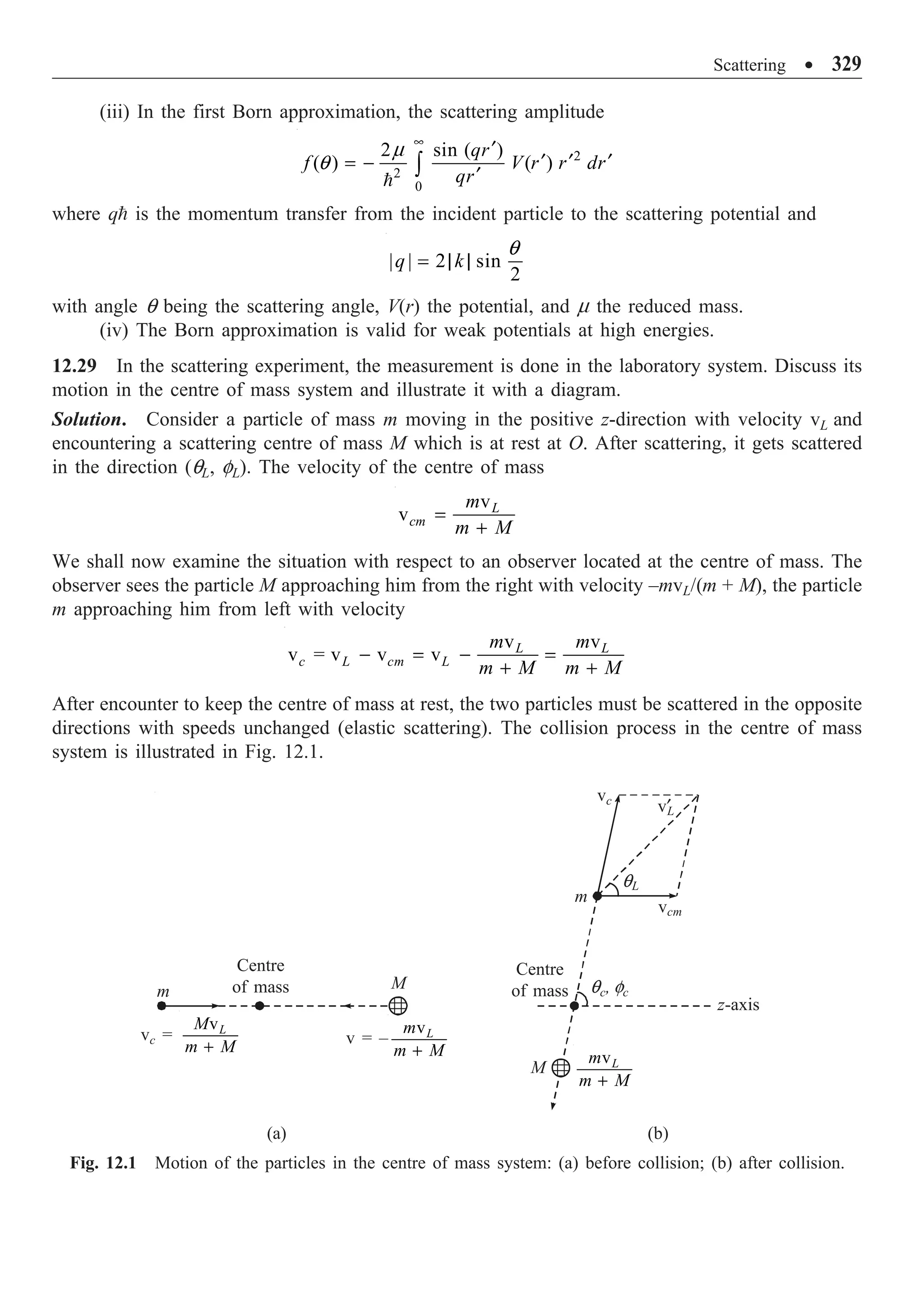
344. 334 ∑ Quantum Mechanics: 500 Problems with Solutions
j(r, t) = cY†
aY, jx = cY†
axY
jx =
1
2
1 2 3 4
3
4
0 0 0 1
0 0 1 0
* * * *
( )
0 1 0 0
1 0 0 0
c
Y
Ê ˆ
Ê ˆ
Á ˜
Á ˜ Y
Á ˜
Á ˜
Y Y Y Y
Á ˜
Á ˜ Y
Á ˜
Á ˜
Á ˜ Á ˜
Y
Ë ¯ Ë ¯
=
4
3
1 2 3 4
2
1
* * * *
( )
c
Y
Ê ˆ
Á ˜
Y
Á ˜
Y Y Y Y
Á ˜
Y
Á ˜
Á ˜
Y
Ë ¯
= 1 4 2 3 3 2 4 1
* * * *
( )
c Y Y + Y Y + Y Y + Y Y
Proceeding on a similar line, we have
jy = 1 4 2 3 3 2 4 1
* * * *
( )
ic -Y Y + Y Y - Y Y + Y Y
jz = 1 3 2 4 3 1 4 2
* * * *
( )
c Y Y - Y Y + Y Y - Y Y
13.5 Prove that the operator ca, where a stands for Dirac matrix, can be interpreted as the velocity
operator.
Solution. In the Heisenberg picture, the equation of motion of the position vector r, which has no
explicit time dependence, is given by
1
[ , ],
d
H
dt i
=
r
r H = ca ◊ p + bmc2
Since a commutes with x, the x-component of the above equation reduces to
dx
dt
=
1 1
[ , ] ( ) ( )
x x x x
c
H xH Hx x p p x
i i i
= - = -
a a
x
= ( )
x x x x
c
xp p x c
i
- =
a a
Similarly,
dy
dt
= cay,
dz
dt
= caz
Thus, ca is the velocity vector.
13.6 Show that (a ◊ A) (a ◊ B) = (A ◊ B) + is ¢ ◊ (A ¥ B), where A and B commute with a and
s ¢ =
0
.
0
s
s
Ê ˆ
Á ˜
Ë ¯
Solution.
(a ◊ A) (a ◊ B) = (ax Ax + ay Ay + az Az) (axBx + ayBy + azBz)
= 2
x
a AxBx + 2
y
a AyBy + 2
z
a AzBz + axay AxBy + axazAxBz
+ ayaxAyBx + ayazAyBz + azaxAzBx + azayAzBy

345. Relativistic Equations ∑ 335
Since 2 2 2
1,
x y z x y y x
= = = = -
a a a a a a a and the cyclic relations
(a ◊ A) (a ◊ B) = (A ◊ B) + axay (AxBy – AyBx) + ayaz (AyBz – AzBy)
+ azax (AzBx – AxBz)
axay =
0 0 0
0
0 0 0
0
y x y z
x
z
y x y z
x
i i
Ê ˆ Ê ˆ Ê ˆ
Ê ˆ
¢
= = =
Á ˜ Á ˜ Á ˜
Á ˜
Ë ¯ Ë ¯
Ë ¯ Ë ¯
s s s s
s
s
s s s s
s
Using this results and the cyclic relations, we get
(a ◊ A)(a ◊ B) = (A ◊ B) + is ¢ ◊ (A ¥ B)
13.7 Consider the one-dimensional Dirac equation
2
[ ( )]
z
i c p mc V z
t
∂
= + +
∂
y
a b y , z
p i
z
∂
= -
∂
0
,
0
z
z
Ê ˆ
= Á ˜
Ë ¯
s
a
s
1 0
,
0 1
z
Ê ˆ
= Á ˜
-
Ë ¯
s
0
0
I
I
Ê ˆ
= Á ˜
-
Ë ¯
b
Show that
(i)
0
0
z
z
Ê ˆ
= Á ˜
Ë ¯
s
s
s
commutes with H; (ii) The one-dimensional Dirac equation can be written as two coupled first order
differential equations.
Solution. The Hamiltonian
2
( )
H c i mc V z
z
∂
Ê ˆ
= - + +
Á ˜
∂
Ë ¯
a b
The commutator
[s, a] =
0 0 0 0 0 0
0 0 0 0 0 0
z z z z z z
z z z z z z
È ˘
Ê ˆ Ê ˆ Ê ˆ Ê ˆ Ê ˆ Ê ˆ
= -
Í ˙
Á ˜ Á ˜ Á ˜ Á ˜ Á ˜ Á ˜
Ë ¯ Ë ¯ Ë ¯ Ë ¯ Ë ¯ Ë ¯
Í ˙
Î ˚
s s s s s s
s s s s s s
=
2 2
2 2
0 0
0
0 0
z z
z z
Ê ˆ Ê ˆ
- =
Á ˜ Á ˜
Ë ¯ Ë ¯
s s
s s
Similarly,
0 0
[ , ] , 0
0 0
z
z
I
I
È ˘
Ê ˆ Ê ˆ
= =
Í ˙
Á ˜ Á ˜
-
Ë ¯
Ë ¯
Í ˙
Î ˚
s
s b
s
Hence,
2
[ , ] [ , ] [ , ] 0
z
H c p mc
= + =
s s a s b

346. 336 ∑ Quantum Mechanics: 500 Problems with Solutions
As [s, H] = 0, the two operators s and H have common eigenfunctions s is a diagonal matrix whose
eigenfunction is
1
2
3
4
Ê ˆ
Á ˜
Á ˜
Á ˜
Á ˜
Á ˜
Ë ¯
y
y
y
y
1 1 1 1
2 2 2 2
3 3 3 3
4 4 4 4
0
1 0 0 0
0 1 0 0 0
0
0 0 1 0
0 0 0 1 0
Ê ˆ Ê ˆ Ê ˆ Ê ˆ
Ê ˆ Ê ˆ
Á ˜ Á ˜ Á ˜ Á ˜
Á ˜ Á ˜
-
-
Á ˜ Á ˜ Á ˜ Á ˜
Á ˜ Á ˜
= = = -
Á ˜ Á ˜ Á ˜ Á ˜
Á ˜ Á ˜
Á ˜ Á ˜ Á ˜ Á ˜
Á ˜ Á ˜
Á ˜ Á ˜
Á ˜ Á ˜ Á ˜ Á ˜
-
-
Ë ¯ Ë ¯
Ë ¯ Ë ¯ Ë ¯ Ë ¯
y y y y
y y y y
s
y y y y
y y y y
From the form of s, it is obvious that
1
3
0
0
Ê ˆ
Á ˜
Á ˜
Á ˜
Á ˜
Á ˜
Ë ¯
y
y
and
2
4
0
0
Ê ˆ
Á ˜
Á ˜
Á ˜
Á ˜
Á ˜
Ë ¯
y
y
are the eigenfunctions of s with the eigenvalues +1 and –1, respectively. Substituting these functions
in the Dirac equation, we get
1 1
2
3 3
0 0
0 0
i i c mc V
t z
Ê ˆ Ê ˆ
Á ˜ Á ˜
∂ ∂
Ê ˆ
Á ˜ Á ˜
= - + +
Á ˜
∂ ∂
Á ˜ Á ˜
Ë ¯
Á ˜ Á ˜
Á ˜ Á ˜
Ë ¯ Ë ¯
y y
a b
y y
2 2
2
4 4
0 0
0 0
i i c mc V
t z
Ê ˆ Ê ˆ
Á ˜ Á ˜
∂ ∂
Ê ˆ
Á ˜ Á ˜
= - + +
Á ˜
Á ˜ Á ˜
∂ ∂
Ë ¯
Á ˜ Á ˜
Á ˜ Á ˜
Ë ¯ Ë ¯
y y
a b
y y
1 1 3
3 3 1
/ 0 0 1 0 /
0 0 0 0 1 0 0
/ 1 0 0 0 /
0 0 1 0 0 0 0
z z
z
z z
y y y
a
y y y
∂ ∂ ∂ ∂
Ê ˆ Ê ˆ Ê ˆ Ê ˆ
Á ˜ Á ˜ Á ˜ Á ˜
- ∂
Á ˜ Á ˜ Á ˜ Á ˜
= =
∂
Á ˜ Á ˜ Á ˜ Á ˜
∂ ∂ ∂ ∂
Á ˜ Á ˜ Á ˜ Á ˜
Á ˜ Á ˜ Á ˜ Á ˜
-
Ë ¯ Ë ¯ Ë ¯ Ë ¯
1 1 1
3 3 3
1 0 0 0
0 0 1 0 0 0 0
0 0 1 0
0 0 0 0 1 0 0
Ê ˆ Ê ˆ Ê ˆ Ê ˆ
Á ˜ Á ˜ Á ˜ Á ˜
Á ˜ Á ˜ Á ˜ Á ˜
= =
Á ˜ Á ˜ Á ˜ Á ˜
- -
Á ˜ Á ˜ Á ˜ Á ˜
Á ˜ Á ˜ Á ˜ Á ˜
-
Ë ¯ Ë ¯ Ë ¯ Ë ¯
y y y
b
y y y

347. Relativistic Equations ∑ 337
Similarly,
2 2 4
4 4 2
0 0 0
0 0 1 0
/ /
0 0 0 1
0 0 0
1 0 0 0
/ /
0 1 0 0
z z
z
z z
y y y
a
y y y
Ê ˆ Ê ˆ Ê ˆ
Ê ˆ
Á ˜ Á ˜ Á ˜
Á ˜
∂ ∂ ∂ ∂ -
- ∂
Á ˜ Á ˜ Á ˜
Á ˜
= =
Á ˜ Á ˜ Á ˜
∂
Á ˜
Á ˜ Á ˜ Á ˜
Á ˜
Á ˜
Á ˜ Á ˜ Á ˜
∂ ∂ ∂ ∂ -
-
Ë ¯
Ë ¯ Ë ¯ Ë ¯
Substituting this equation in the Dirac equations, we have
1 3 1 1
2
3 1 3 3
0 0 0 0
( )
0 0 0 0
i i c mc V z
t z
Ê ˆ Ê ˆ Ê ˆ Ê ˆ
Á ˜ Á ˜ Á ˜ Á ˜
∂ ∂
Á ˜ Á ˜ Á ˜ Á ˜
= - + +
∂ ∂
Á ˜ Á ˜ Á ˜ Á ˜
-
Á ˜ Á ˜ Á ˜ Á ˜
Á ˜ Á ˜ Á ˜ Á ˜
Ë ¯ Ë ¯ Ë ¯ Ë ¯
y y y y
y y y y
2 4 2 2
2
4 2 4 4
0 0 0 0
( )
0 0 0 0
i i c mc V z
t z
Ê ˆ Ê ˆ Ê ˆ Ê ˆ
Á ˜ Á ˜ Á ˜ Á ˜
- -
∂ ∂
Á ˜ Á ˜ Á ˜ Á ˜
= - + +
Á ˜ Á ˜ Á ˜ Á ˜
∂ ∂
Á ˜ Á ˜ Á ˜ Á ˜
Á ˜ Á ˜ Á ˜ Á ˜
- -
Ë ¯ Ë ¯ Ë ¯ Ë ¯
y y y y
y y y y
Each of these two equations represents two coupled differential equations.
13.8 For a Dirac particle moving in a central potential, show that the orbital angular momentum
is not a constant of motion.
Solution. In the Heisenberg picture, the time rate of change of the L = r ¥ p is given by
[ , ]
d
i L H
dt
=
L
Its x-component is
2
[ , ] [ , ]
x x z y
d
i L L H yp zp c mc
dt
a
= = - ◊ +
b
p
Since a and b commute with r and p,
x
d
i L
dt
= [ , ] [ , ]
z y y y z z
yp c zp c
-
a a
p p
= [ , ] [ , ]
y z y z y z
c y p p c z p p
-
a a
= cipzay – cipyaz
= ic (pza – pyaz)
which shows that Lx is not a constant of motion. Similar relations hold good for Ly and Lz
components. Hence the orbital angular momentum L is not a constant of motion.
13.9 Prove that the quatity L + (1/2)s ¢, where L is the orbital angular momentum of a particle,
and s ¢ =
0
0
s
s
¢
Ê ˆ
Á ˜
¢
Ë ¯
is a constant of motion for the particle in Dirac’s formalism. Hence give an
interpretation for the additional angular momentum 1/2 s ¢.

348. 338 ∑ Quantum Mechanics: 500 Problems with Solutions
Solution. In Dirac’s formalism, the Hamiltonian of a free particle is
H = ca ◊ p + bmc2
(i)
In the Heisenberg picture, the equation of motion for an operator M is given by
[ , ]
d
i H
dt
=
M M (ii)
Hence, for a dynamical variable to be a constant of motion, it should commute with its Hamiltonian.
Writing
1
2
¢
= + s
M L (iii)
where equation of motion is
2
1 1
,
2 2
d
i c mc
dt
a
Ê ˆ È ˘
¢ ¢
+ = + ◊ +
Á ˜ Í ˙
Ë ¯ Î ˚
s s b
L L p (iv)
The x-component of Eq. (iv) is
1
2
x x
d
i L
dt
Ê ˆ
¢
+
Á ˜
Ë ¯
s =
2
1
,
2
x x
L c mc
a
È ˘
¢
+ ◊ +
Í ˙
Î ˚
s b
p
= 2 2
1
[ , ] [ , ]
2
x x
L c mc c mc
a a
¢
◊ + + ◊ +
b s b
p p (v)
Let us now evaluate the commutators on the right side of (v) one by one
2 2
[ , ] [ , ]
x z y x x y y z z
L c mc yp zp c p c p c p mc
a ◊ + = - + + +
b a a a b
p
Since a and b commute with r and p,
2
[ , ]
x
L c mc
a ◊ + b
p = [ , ] [ , ]
z y y z z z
yp c p zp c p
-
a a
= [ , ] [ , ]
y z y z y z
c y p p c z p p
-
a a
= ( )
y z z y
ic p p
-
a a (vi)
The second commutator in Eq. (v) is
2
[ , ]
x c mc
a
¢ ◊ +
s b
p = 2
[ , ]
x x x y y z z
c p c p c p mc
¢ + + +
s a a a b
= 2
[ , ] [ , ] [ , ] [ , ]
x x x x y y x z z x
c p c p c p mc
¢ ¢ ¢ ¢
+ + +
s a s a s a s b
From Problem 13, we have
[ , ] 0,
x
¢ =
s b [ , ] 0,
x x
¢ =
s a [ , ] 2 ,
x y z
i
¢ =
s a a [ , ] 2
x z y
i
¢ = -
s a a
Substituting these commutators in the above equation, we get
2
[ , ]
x c mc
a
¢ ◊ +
s b
p = [ , ] [ , ]
x y y x z z
c p c p
¢ ¢
+
s a s a
= 2 2
z y y z
ic p ic p
-
a a (vii)

349. Relativistic Equations ∑ 339
From Eqs. (v)–(vii),
1
2
x x
d
i L
dt
Ê ˆ
¢
+
Á ˜
Ë ¯
s =
1
( ) 2 ( )
2
y z z y z y y z
ic p p ic p p
- + ¥ -
a a a a (viii)
= 0
1
2
x x
L ¢
+ s = constant (ix)
Similar relations are obtained for the y- and z-components. Hence,
1
2
s ¢
+
L = constant (x)
From the structure of the s ¢ matrix, we can write
2 2 2
1
x y z
¢ ¢ ¢
= = =
s s s
This gives the eigenvalues of
1
2
s ¢
as +
1
2
or –
1
2
. Thus, the additional angular momentum
1
2
s ¢
can be interpreted as the spin angular momentum, i.e.,
0
1
2 0
s
s
Ê ˆ
= Á ˜
Ë ¯
S
13.10 If the radial momentum pr and radial velocity ar for an electron in a central potential are
defined by
pr = ,
i
r
-
r p
◊
ar =
r
r
a ◊
show that
(a ◊ p) = ar pr + r
i k
r
ba
where k =
( )
.
b ¢ +
L
s ◊
Solution. The relativistic Hamiltonian of an electron in a central potential V(r) is given by
H = c(a ◊ p) + bmc2
+ V(r)
If A and B are operators, then
(a ◊ A)(a ◊ B) = (A ◊ B) + s¢ ◊ (A ¥ B)
Setting A = B = r, we have (a ◊ r)2
= r2
. Taking A = r and B = p, we get
(a ◊ r)(a ◊ p) = (r ◊ p) + is ¢ ◊ L
Given
[( ) ]
k
b ¢ +
=
L
s ◊
or
k
s
b
¢ = -
L
◊

350. 340 ∑ Quantum Mechanics: 500 Problems with Solutions
Substituting this value of s ¢ ◊ L and multiplying by a ◊ r, we obtain
(a ◊ r)2
(a ◊ p) = (a ◊ r) ( )
k
i
b
È ˘
Ê ˆ
+ -
Í ˙
Á ˜
Ë ¯
Î ˚
r p
◊
Since
(a ◊ r)2
= r2
we have
2
( )
( )
ik i ik
i
r r r
r b b
-
È ˘ È ˘
= - + = +
Í ˙ Í ˙
Î ˚ Î ˚
a r a r r p
a p r p
◊ ◊ ◊
◊ ◊
Using the definitions of pr and ar, we get
a ◊ p =
2
r r
r r r r
i k i k
p p
r r
+ = +
a b a
a a
b b
= r
r r
i k
p
r
+
ba
a
13.11 If one wants to write the relativistic energy E of a free particle as
2
2
E
c
= (a ◊ p + bmc)2
,
show that a’s and b’s have to be matrices and establish that they are nonsingular and Hermitian.
Solution. The relativistic energy (E) of a free particle is given by
E2
= c2
p2
+ m2
c4
= c2
(p2
+ m2
c2
)
When E2
/c2
is written as given in the problem,
p2
+ m2
c2
= (a ◊ p + bmc)2
= 2 2 2 2 2 2
x x y y z z
p p p
+ +
a a a
+ 2 2 2
( ) ( )
x y y x x y x z z x x z
m c p p p p
+ + + +
b a a a a a a a a
+ ( ) ( )
y z z y y z x x x
p p mcp
+ + +
a a a a a b ba
+ ( ) ( )
y y y z z z
mcp mcp
+ + +
a b ba a b ba
For this equation to be valid, it is necessary that
2 2 2 2
1,
x y z
= = = =
a a a b [ , ] 0, [ , ] 0
x y y z
+ +
= =
a a a a
[ , ] 0, [ , ] 0
x z x
+ +
= =
a a a b , [ , ] 0, [ , ] 0
y z
+ +
= =
a b a b
It is obvious that the a’s and b cannot be ordinary numbers. The anticommuting nature of the a’s
and b suggests that they have to be matrices. Since the squares of these matrices are unit matrices,
they are nonsingular. As the a’s and b determine the Hamiltonian, they must be Hermitian.

351. Relativistic Equations ∑ 341
13.12 If s ¢ =
0
0
s
s
Ê ˆ
Á ˜
Ë ¯
, show that
(i) 2 2 2
1.
x y z
¢ ¢ ¢
= = =
s s s
(ii) [ , ] 0,
x x
¢ =
s a [ , ] 2 ,
x y z
i
¢ =
s a a [ , ] 2
x z y
i
¢ = -
s a a ,
where s is the Pauli matrix and ax, ay, az are the Dirac matrices.
Solution.
0
,
0
s
s
s
Ê ˆ
¢ = Á ˜
Ë ¯
0
0
x
x
x
Ê ˆ
¢ = Á ˜
Ë ¯
s
s
s
(i)
2
2
2
0 0 1 0
0
0 0 0 1
0
x x x
x
x x x
Ê ˆ
Ê ˆ Ê ˆ Ê ˆ
¢ = = =
Á ˜
Á ˜ Á ˜ Á ˜
Ë ¯
Ë ¯ Ë ¯ Ë ¯
s s s
s
s s s
A similar procedure gives the values of 2
y
¢
s and 2
z
¢
s . Hence the result
(ii) [ , ]
x x
¢
s a =
0 0 0 0
0 0 0 0
x x x x
x x x x
Ê ˆ Ê ˆ Ê ˆ Ê ˆ
-
Á ˜ Á ˜ Á ˜ Á ˜
Ë ¯ Ë ¯ Ë ¯ Ë ¯
s s s s
s s s s
=
2 2
2 2
0 0
0
0 0
x x
x x
Ê ˆ Ê ˆ
- =
Á ˜ Á ˜
Ë ¯ Ë ¯
s s
s s
[ , ]
x y
¢
s a =
0 0
0 0
0 0
0 0
y y
x x
y y
x x
Ê ˆ Ê ˆ
Ê ˆ Ê ˆ
-
Á ˜ Á ˜
Á ˜ Á ˜
Ë ¯ Ë ¯
Ë ¯ Ë ¯
s s
s s
s s
s s
0 0
0 0
x y y x
x y y x
Ê ˆ Ê ˆ
-
Á ˜ Á ˜
Ë ¯ Ë ¯
s s s s
s s s s
=
0
0
x y y x
x y y x
-
Ê ˆ
Á ˜
-
Ë ¯
s s s s
s s s s
=
0 2
2
2 0
z
z
z
i
i
i
Ê ˆ
=
Á ˜
Ë ¯
s
a
s
Proof of the other relation is straightforward.
13.13 Show that matrix
0
0
s
s
s
Ê ˆ
¢ = Á ˜
Ë ¯
is not a constant of motion.
Solution. The equation of motion of s ¢ in the Heisenberg picture is
[ , ]
d
i H
dt
s
s
¢
¢
=
Hence for s ¢ to be a constant of motion, ,
x y
¢ ¢
s s and z
¢
s should commute with the Hamiltonian.
Thus,
2
[ , ] [ , ]
x x
H c mc
¢ ¢
= ◊ +
s s b
a p

352. 342 ∑ Quantum Mechanics: 500 Problems with Solutions
Since x
¢
s commutes with b,
[ , ] , , ,
x x x x x y y x z z
H c p c p c p
s s a s a s a
Í ˙
¢ ¢ ¢ ¢
È ˘
= + +
È ˘
Î ˚ Î ˚
Î ˚
From Problem 13.12,
, 0,
x x
¢ =
È ˘
Î ˚
s a , 2 ,
x y z
i
Í ˙
¢ =
Î ˚
s a a , 2
x z y
i
¢
È ˘ = -
Î ˚
s a a
, 2 ( ) 0
x z y y z
H ic p p
¢ = - π
È ˘
Î ˚
s a a
Hence the result.
13.14 Show that Dirac’s Hamiltonian for a free particle commutes with the operator s ◊ p, where
p is the momentum operator and s is the Pauli spin operator in the space of four component spinors.
Solution. Dirac’s Hamiltonian for a free particle is
2
( )
H c mc
= ◊ + b
a p
where
0
,
0
s
s
Ê ˆ
= Á ˜
Ë ¯
a
0
0
I
I
Ê ˆ
= Á ˜
-
Ë ¯
b
0 0
0 0
s s
a
s s
◊
Ê ˆ Ê ˆ
◊ = ◊ =
Á ˜ Á ˜
◊
Ë ¯ Ë ¯
p
p p
p
0
0
I
s
s s
s
◊
Ê ˆ
◊ = ◊ = Á ˜
◊
Ë ¯
p
p p
p
[s ◊ p, H] = [s ◊ p, ca ◊ p + bmc2
]
= c [(s ◊ p), a ◊ p] + [s ◊ p, bmc2
]
= 2
0 0 0 1 0
, ,
0 0 0 0 1
c mc
s s s
s s s
È ˘ È ˘
◊ ◊ ◊
Ê ˆ Ê ˆ Ê ˆ Ê ˆ
+
Í ˙ Í ˙
Á ˜ Á ˜ Á ˜ Á ˜
◊ ◊ ◊ -
Ë ¯ Ë ¯ Ë ¯ Ë ¯
Í ˙ Í ˙
Î ˚ Î ˚
p p p
p p p
= 0 + 0 = 0
Hence the result.

353. 343
With the advent of quantum mechanics, elegant methods were developed to study the mechanism that
holds the atoms together in molecules. The molecular orbital (MO) and valence bond (VB) methods
are the two commonly used methods. Recent computational works mainly use the MO methods.
14.1 Born–Oppenheimer Approximation
In molecules, one has to deal with not only the moving electrons but also the moving nuclei. Born
and Oppenheimer assumed the nuclei as stationary and in such a case, the Hamiltonian representing
the electronic motion is
2
2
2 2
2
2 i
i ij
i i i j i
kz z e
kz e ke
H
m r r r
a b
a
a ab
a a b a
= - — - + +
 Â Â   (14.1)
where i, j refer to electrons, a, b to nuclei and k = 1/(4p e0).
14.2 Molecular Orbital and Valence Bond Methods
In the molecular orbital method, developed by Mulliken, molecular wavefunctions, called molecular
orbitals, are derived first. In the commonly used approach, the molecular orbital y is written as a
linear combination of the atomic orbitals (LCAO) as
1 1 2 2
c c
= + + …
y y y (14.2)
where y1, y2, º are the individual atomic orbitals. The constants c1, c2, º are to be selected in such
a way that the energy given by y is minimum.
In the valence bond approach, atoms are assumed to maintain their individual identity in a
molecule and the bond arises due to the interaction of the valence electrons. That is, a bond is formed
when a valence electron in an atomic orbital pairs its spin with that of another valence electron in
the other atomic orbital.
Chemical Bonding
CHAPTER 14

354. 344 ∑ Quantum Mechanics: 500 Problems with Solutions
14.3 Hydrogen Molecule-ion
Hydrogen molecule-ion consists of an electron of charge –e associated with two protons a and b
separated by a distance R (see Fig. 14.1). The electron’s atomic orbital, when it is in the
neighbourhood of a is
1/2
a
a 3
0
0
1
exp
r
a
a
y
p
Ê ˆ -
Ê ˆ
= Á ˜ Á ˜
Ë ¯
Ë ¯
(14.3)
ra rb
a b
R
e_
and when it is in the neighbourhood of b, it is
1/2
b
b 3
0
0
1
exp
r
a
a
y
p
Ê ˆ -
Ê ˆ
= Á ˜ Á ˜
Ë ¯
Ë ¯
(14.4)
A reasonable MO will be
y = c1ya + c2ya (14.5)
where c1 and c2 are constants. Then the energy E of the system is given by
H
E
· | | Ò
=
· | Ò
y y
y y
(14.6)
Substituting the value of y and simplifying, we get the energies as
2
aa ab
1
1
H
V V ke
E E
S R
+
= - +
+
(14.7)
2
aa ab
2
1
H
V V ke
E E
S R
-
= - +
-
(14.8)
where
2
aa a a
b
,
ke
V
r
y y
=
2
ab a b
a
ke
V
r
y y
= (14.9)
a b b a
| |
S y y y y
= · Ò = · Ò (14.10)
Fig. 14.1 The H+
2 molecule.

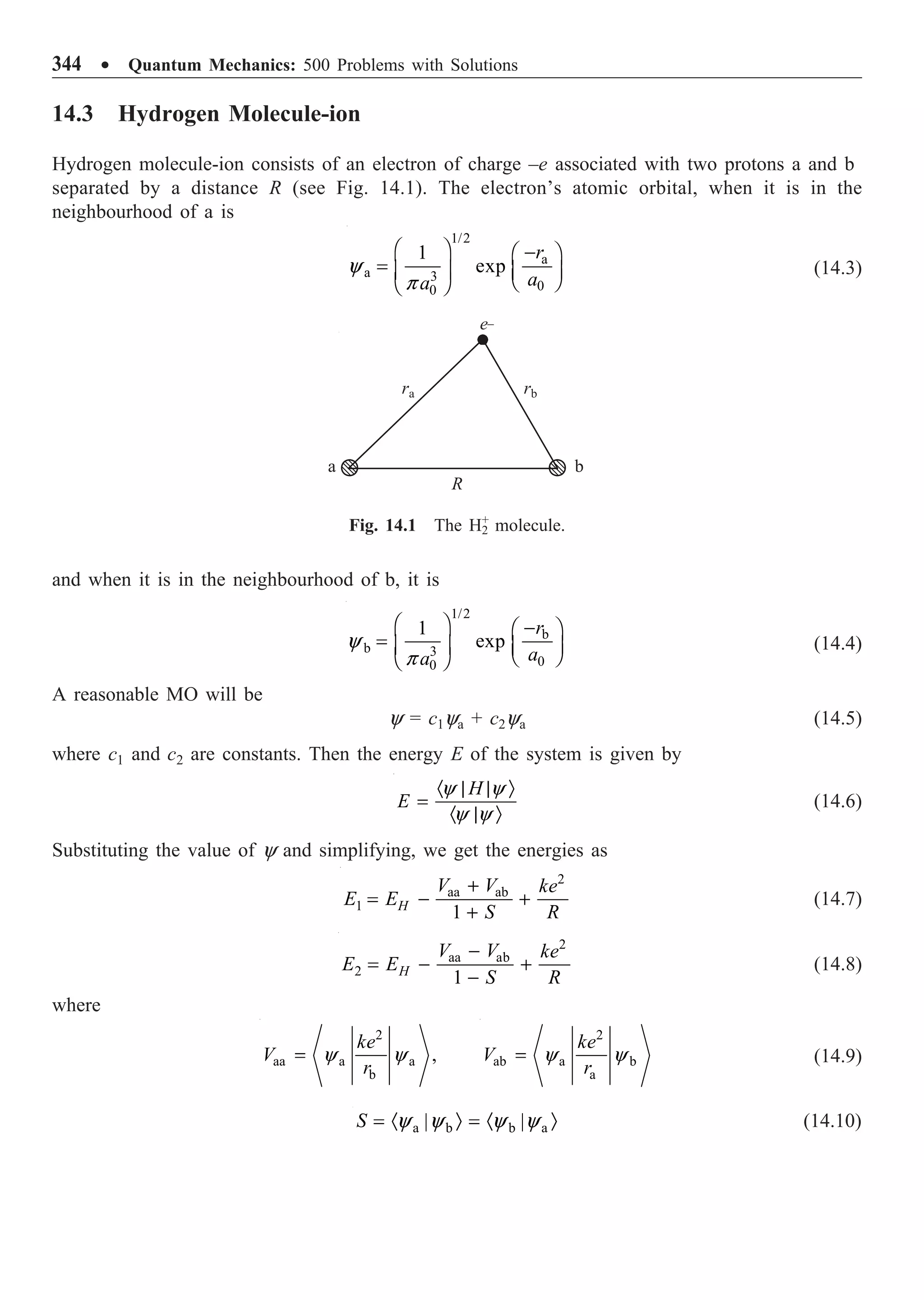
355. Chemical Bonding ∑ 345
The normalized wavefunctions corresponding to these energies are
a b
1 ,
2 2S
y y
y
+
=
+
a b
2
2 2S
y y
y
-
=
-
(14.11)
The wavefunction y1 corresponds to a build-up of electron density between the two nuclei and is
therefore called a bonding molecular orbital. The wavefunction y2 is called an antibonding orbital
since it corresponds to a depletion of charge between the nuclei.
14.4 MO Treatment of Hydrogen Molecule
In MO theory the treatment of hydrogen molecule is essentially the same as that of H+
2 molecule.
One can reasonably take that in the ground state both the electrons occupy the bonding orbital y1
(Eq. 14.1) of H+
2 which is symmetric with respect to interchange of nuclei. The trial wave function
of H2 molecule can then be taken as
a b a b
mo 1 1
[ (1) (1)] [ (2) (2)]
(1) (2)
2 (1 )
S
+ +
= =
+
y y y y
y y y (14.12)
With this wave function, the energy is calculated.
14.5 Diatomic Molecular Orbitals
Figure 14.2 illustrates the formation of bonding and antibonding orbitals from two 1s atomic orbitals.
Both are symmetrical about the internuclear axis. Molecular orbitals which are symmetrical about the
internuclear axis are designated by s (sigma) bond, and those which are not symmetrical about
the internuclear axis are designated by p (pi) bond. The bonding orbital discussed is represented by
the symbol 1ss since it is produced from two 1s atomic orbitals. The antibonding state is represented
by the symbol 1ss *, the asterisk representing higher energy.
ya(1s) + yb(1s)
ya(1s) – yb(1s)
a
+
b
+
a
+
b
a
+
b
–
a
+
b
–
(a)
(b)
Fig. 14.2 Combination of 1s orbitals to form (a) bonding orbital 1ss, and (b) antibonding orbital 1ss*.

356. 346 ∑ Quantum Mechanics: 500 Problems with Solutions
If an inversion of a molecular orbital about the centre of symmetry does not change the sign
of y, it is said to be even and is denoted by the symbol g as a subscript. If the sign changes, the
orbital is said to be odd and a subscript u is assigned to the symbol. In this notation, the bonding
and antibonding orbitals are respectively denoted by 1ssg and 1ssu
*. Two 2s atomic orbitals combine
to form again a bonding 2ssg and an antibonding 2ssu
* molecular orbitals. The terminology followed
for labelling MOs in the increasing order of energy is
1s 1s * 2s 2s * 2p (2p 2p ) (2p * 2p *) 2p *
x y z y z x
s s s s s p = p p = p s (14.13)

357. Chemical Bonding ∑ 347
PROBLEMS
14.1 Illustrate, with the help of diagrams the combination of two p-orbitals, bringing out the
formation of bonding sg, antibonding su
*, bonding pu and antibonding pu
* orbitals.
Solution. The two lobes of each of the p-orbitals have opposite signs. If the internuclear axis is
taken as the x-direction, two px atomic orbitals combine to give the molecular orbitals 2pxsg and
2pxsu
*, which is illustrated in Fig. 14.3 Both have symmetry about the bond axis. The combination
Atomic Orbitals Molecular Orbitals
ya(px) – yb(px)
2pxsg
a b
– + + –
– + –
ya(px) + yb(px)
2pxsu
*
a b
– + – +
– + +
–
(a)
(b)
Fig. 14.3 Formation of (a) bonding orbital 2pxsg, and (b) antibonding 2pxsu
* molecular orbitals from two px
orbitals.
of two py orbitals gives the molecular orbitals 2pypu and 2pypg
*, see Fig. 14.4. The pypu MO consists
of two streamers, one above and one below the nuclei. In this case, the bonding orbital is odd and
the antibonding orbital is even, unlike the earlier ones. Formation of p molecular orbitals from
atomic pz orbitals is similar to the one from atomic py orbitals.
Atomic Orbitals Molecular Orbitals
fi
fi
ya(py) + yb(py) 2py pu
fi
fi
ya(py) – yb(py) 2py pg
*
Fig. 14.4 The formation of (a) bonding orbital 2pypu, and (b) antibonding 2pypg
* from two 2py orbitals.
+ +
– –
+ –
– +
+
–
+
–
–
+

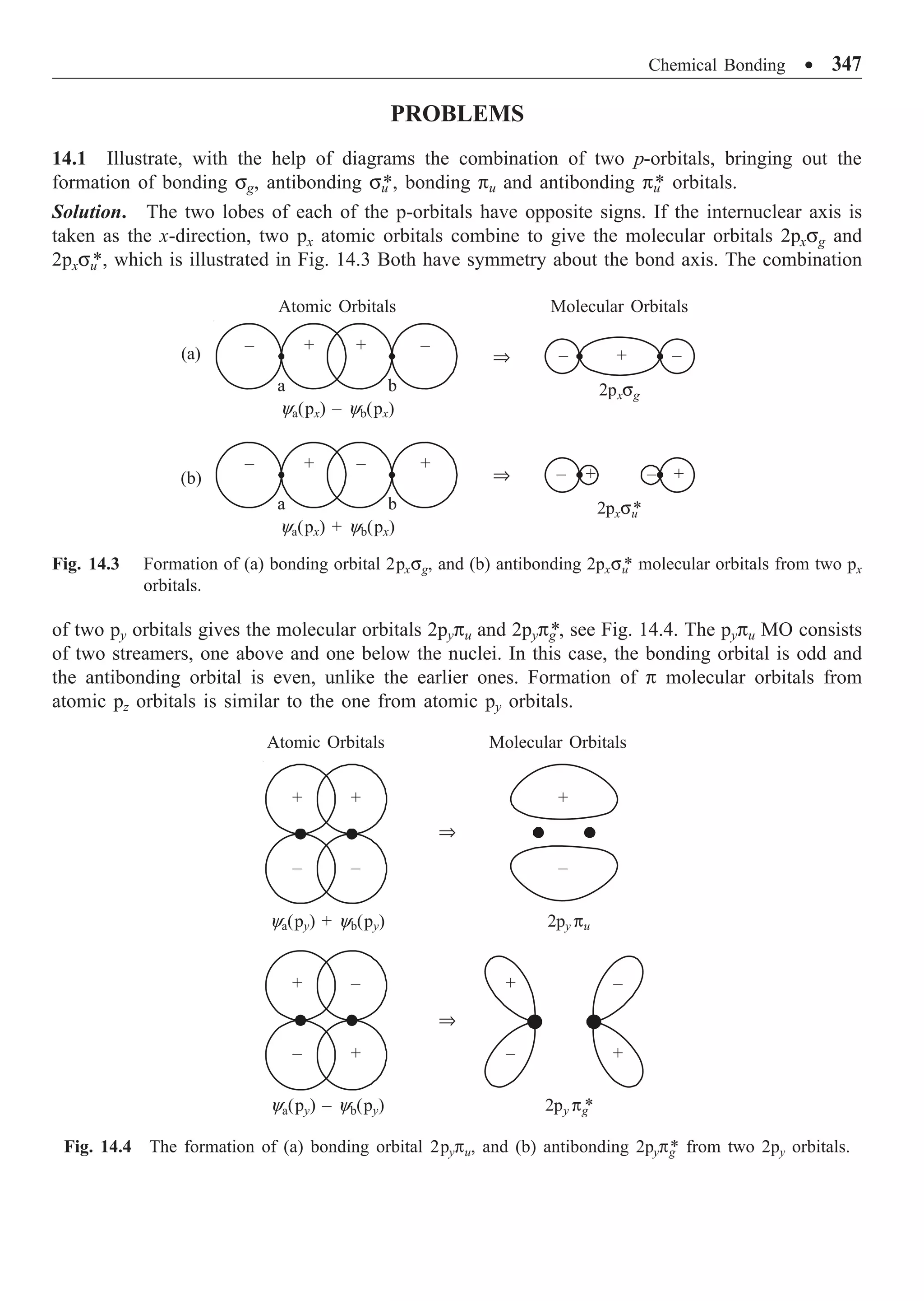
358. 348 ∑ Quantum Mechanics: 500 Problems with Solutions
14.2 Outline the Heitler-London wavefunctions for hydrogen molecule. What are singlet and triplet
states of hydrogen?
Solution. Hydrogen molecule is a system of two hydrogen atoms and, therefore, can be described
by the wave function
y(1, 2) = ya(1) yb(2) (i)
where a and b refer to the two nuclei, 1 and 2 to the two electrons. The function ya(1) yb(2) means
electron 1 is associated with the atom whose nucleus is a and electron 2 is associated with the atom
whose nucleus is b. The electrons are indistinguishable. Hence,
y(2, 1) = ya(2) yb(1) (ii)
is also a wave function. The wave function of the two-electron system is a linear combination of the
two.
Since an exchange of electron 1 and electron 2 leaves the Hamiltonian of the system
unchanged, the wavefunctions must either be symmetric or antisymmetric with respect to such an
exchange. The symmetric ys and antisymmetric yas combinations are
ys = Ns [ya(1) yb(2) + ya(2) yb(1)] (iii)
yas = Nas [ya(1) yb(2) – ya(2) yb(1)] (iv)
where Ns and Nas are normalization constants. The spin functions of a two-spin half system is given
by
as
1
[ (1) (2) (1) (2)]
2
= -
c a b b a (v)
s
(1) (2)
1
[ (1) (2) (1) (2)]
2
(1) (2)
Ï
Ô
Ô
= +
Ì
Ô
Ô
Ó
a a
c a b b a
b b
(vi)
As the total wave function has to be antisymmetric, the symmetric space part combines with the
antisymmetric spin part and vice versa. Hence, the inclusion of electron spin leads to the Heitler-
London wave functions
s a b a b
1
[ (1) (2) (2) (1)] [ (1) (2) (1) (2)]
2
N + -
y y y y a b b a (vii)
as a b a b
(1) (2)
1
[ (1) (2) (2) (1)] [ (1) (2) (1) (2)]
2
(1) (2)
N
Ï
Ô
Ô
- = +
Ì
Ô
Ô
Ó
a a
y y y y a b b a
b b
(viii)
Equation (vii) corresponds to a singlet state since S = 0, whereas Eq. (viii) is a triplet state as
S = 1.

359. Chemical Bonding ∑ 349
14.3 In the hydrogen molecule ion, the wave functions corresponding to energy E1 and E2 are
y1 = c1(ya + yb) and y2 = c2(ya – yb), where ya and yb are hydrogenic wave functions. Normalize
the functions. What will be the normalization factor if the two nuclei are at infinite distance?
Solution. Given
y1 = c1(ya + yb), y2 = c2(ya – yb)
The normalization of y1 gives
2
1 a b a b
| | ( )|( )
c · + + Ò
y y y y = 1
2
1 a a b b a b b a
| | [ | | | | ]
c · Ò + · Ò + · Ò + · Ò
y y y y y y y y = 1
Writing a b b a
| | ,
· Ò = · Ò
y y y y refer Eq. (14.10), we get
c1
2
[1 + 1 + S + S] = 1
c1 =
1
,
2 2S
+
y1 = a b
2 2S
+
+
y y
Normalization of y2 gives
2
2 a a b b a b b a
| | [ | | | | ]
c · Ò + · Ò - · Ò - · Ò
y y y y y y y y = 1
c2 =
1
,
2 2S
-
y2 = a b
2 2S
-
-
y y
When the two nuclei are at infinite distance, the overlap integral ·ya |ybÒ = ·yb |yaÒ = 0. Hence the
normalization factor for both y1 and y2 is 1/ 2.
14.4 The Heitler-London wave functions for hydrogen molecule are
ys = Ns [ya(1) yb(2) + ya(2) yb(1)]
yas = Na [ya(1) yb(2) – ya(2) yb(1)]
Evaluate the normalization constants Ns and Na. What will be the normalization factor if the nuclear
separation is infinite.
Solution. The normalization condition of the symmetric Heitler-London trial function gives
2
s a b a b a b a b
| | [ (1) (2) (2) (1)]|[ (1) (2) (2) (1)] 1
N · + + Ò =
y y y y y y y y
2
s a b a b a b a b
| | [ (1) (2)| (1) (2) (1) (2)| (2) (1)
N · Ò + · Ò
y y y y y y y y
a b a b a b a b
(2) (1)| (1) (2) (2) (1)| (2) (1) ]
+ · Ò + · Ò
y y y y y y y y = 1
|Ns|2
[1 + S2
+ S2
+ 1] = 1, Ns =
2
1
2 2S
+
since
·ya(1) | ya(1)Ò = ·yb(2) | yb(2)Ò = ·ya(2) | ya(2)Ò = ·yb(1) | yb(1)Ò = 1
·ya(1)yb(2) | ya(2)yb(1)Ò = ·ya(1) | yb(1)Ò ·yb(2) | ya(2)Ò = S ◊ S = S2

360. 350 ∑ Quantum Mechanics: 500 Problems with Solutions
Similarly,
Na =
2
1
2 2S
-
For infinite nuclear separation, S = 0, Ns = Na = 1/ 2 .
14.5 Write the electronic configuration of N2 molecule in the MO concept and explain the
formation of the triple bond N ∫ N.
Solution. The 14 electrons in the nitrogen molecule are distributed as
2 2 2 4
*
KK (2s ) (2s ) (2p ) (2p 2p )
g u x g y z
s s s p = p
The presence of two electrons in the bonding orbital 2ssg and two electrons in the antibondiong
2ssu
* leads to no bonding. The remaining bonding orbitals (2pxsg)2
(2pyp = 2pzp)4
are not cancelled
by the corresponding antibonding orbitals. These six bonding electrons give the triple bond N ∫ N,
one bond being s and the other two are p bonds.
14.6 Write the electronic configuration of O2 and S2 and account for their paramagnetism.
Solution. The sixteen electrons in the O2 molecule are distributed as
2 2 2 4 2
* *
KK (2s ) (2s ) (2p ) (2p ) (2p )
g u g u g
s s s p p
where KK stands for 2 2
*
(1s ) (1s )
g u
s s . The orbital *
2p g
p is degenerate. Hence the two electrons in
that antibonding orbital will go one each with parallel spins (Hund’s rule). Since the last two
electrons are with parallel spins, the net spin is one and the molecule is paramagnetic.
The electronic configuration of S = 1s2
2s2
2p6
3s2
3p4
and, therefore, the electronic
configuration of S2 is
KKLL (3ss)2
(3ss*)2
(3pxs)2
(3py = 3pzp)4
(3pyp* = 3pzp*)2
where LL stands for the n = 2 electrons. The orbitals 3pyp* = 3pzp* can accommodate four electrons.
By Hund’s rule, the two available electrons will enter each of these with their spins parallel, giving
a paramagnetic molecule.
14.7 The removal of an electron from the O2 molecule increases the dissociation energy from
5.08 to 6.48 eV, whereas in N2, the removal of the electron decreases the energy from 9.91 to
8.85 eV. Substantiate.
Solution. The bonding MOs produce charge building between the nuclei, and the antibondig MOs
charge depletion between the nuclei. Hence, removal of an electron from an antibonding MO
increases the dissociation energy De or decreases the bond length of the bond, whereas removal of
an electron from a bonding MO decreases De or increases the bond length. The electronic
configuration of O2 is
2 2 2 4 2
* *
KK (2s ) (2s ) (2p ) (2p 2p ) (2p )
g u x g y u z u g
s s s p = p p
The highest filled MO is antibonding. Hence removal of an electron increases the De from 5.08 to
6.48 eV. The electronic configuration of N2 is
2 2 2 4
*
KK (2s ) (2s ) (2p ) (2p 2p )
g u x g y u z u
s s s p = p

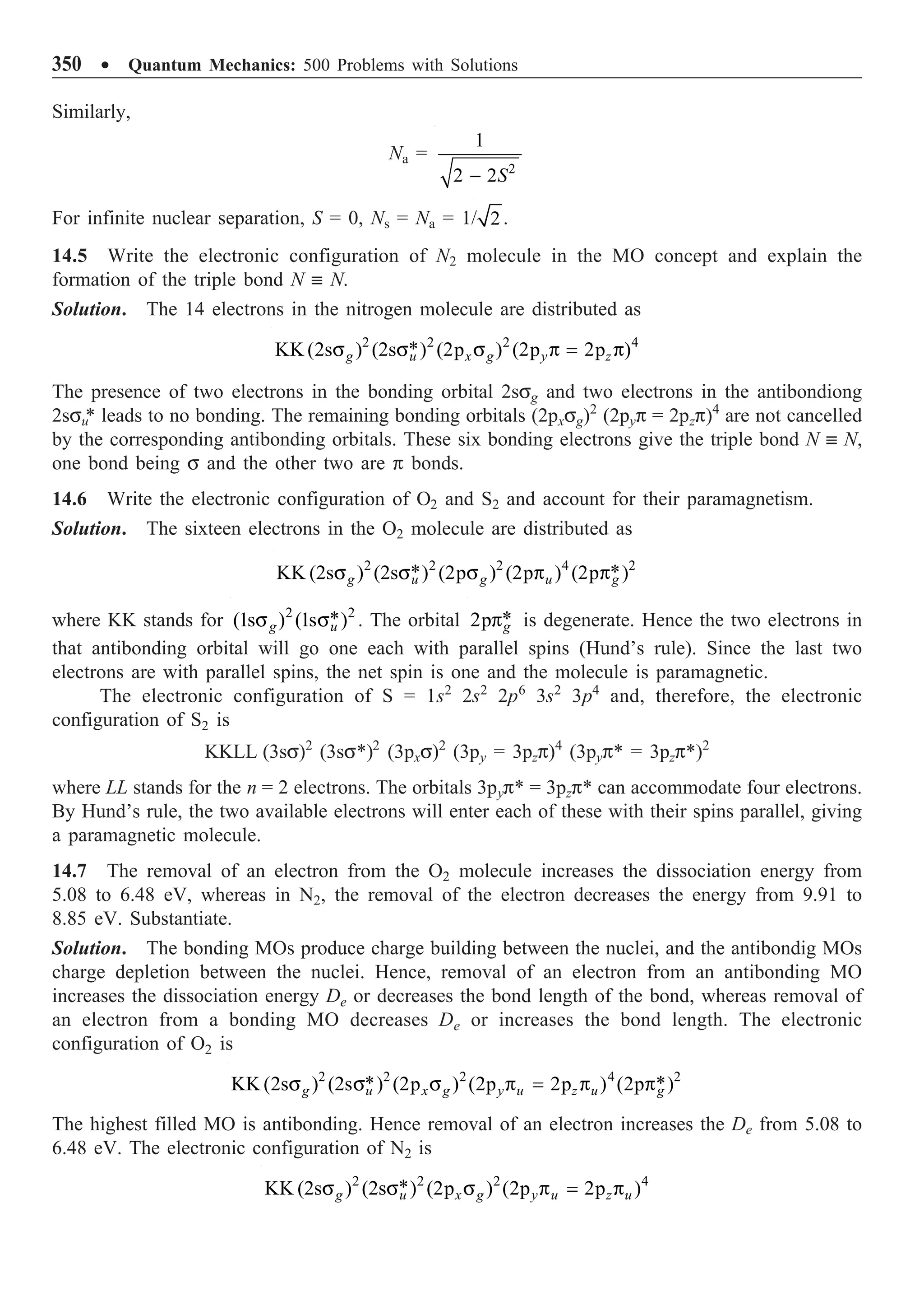
361. Chemical Bonding ∑ 351
Removal of an electron from the highest filled bonding orbital decreases the dissociation
energy from 9.91 to 8.85 eV.
14.8 Discuss the type of bonding in the heteronuclear diatomic molecule NO. Why is the bond in
NO+
expected to be shorter and stronger than that of NO?
Solution. Nitrogen and oxygen are close to each other in the periodic table and, therefore, their
AOs are of similar energy. The nitrogen atom has seven electrons and the oxygen atom eight. The
energy levels of the various MOs are the same as those for homonuclear diatomic molecules.
Therefore, the electronic configuration of NO molecule is
2 2 2 4 1
* *
KK (2s ) (2s ) (2p ) (2p 2p ) (2p )
g u x g y u z u g
s s s p = p p
The inner shell is nonbonding, the bonding and antibonding (2ssg) and (2ssu
*) orbitals cancel.
Though the four electrons in (2pypu = 2pzpu)4
orbital can give two p bonds, a half-bond is cancelled
by the presence of one electron in the antibonding 2ppg
* orbital. This leads to a s-bond (2pxsg)2
a
full p-bond and a half p-bond form 2p electrons. The molecule is paramagnetic since it has an
unpaired electron. Removal of an electron from the system means the removal of an electron from
the antibonding orbital. Hence, the bond in NO+
is expected to be shorter and stronger.
14.9 Compare the MO wavefunction of hydrogen molecule with that of the valence bond theory.
Solution. Equation (14.12) gives the MO wavefunction and the Heitler-London function for
hydrogen molecule is given in Problem 14.4. So,
ymo = constant [ya(1)ya(2) + yb(1)yb(2) + ya(1)yb(2) + yb(1)ya(2)]
yHL = constant [ya(1)yb(2) ± ya(2)yb(1)]
The first two terms in ymo represent the possibility of both the electrons being on the same proton
at the same time.These represent the ionic structures H–
a Hb
+
and Ha
+
H–
b. The third and the fourth
terms represent the possibility in which the electrons are shared equally by both the protons, and
hence they correspond to covalent structures. Both the terms in the valance bond wavefunction
correspond to covalent structures as one electron is associated with one nucleus and the second
electron is associated with the other nucleus.
14.10 Write the electronic configuration of Na2 and S2 molecules in the MO concept.
Solution. The electronic configuration of Na: 1s2
2s2
2p6
3s1
.
The electronic configuration of Na2 molecule is
Na2 [KK (2ss)2
(2ss*
)2
(2pyp = 2pzp)4
(2pxs)2
(2pyp* = 2pzp*)4
(2pxs*)2
(3ss)2
]
= Na2 [KK LL (3ss)2
]
This result may be compared with the electronic configuration of Li2, another alkali metal.
The electronic configuration of S: 1s2
2s2
2p6
3s2
3p4
. The electronic configuration of S2
molecule is
S2 [KK LL (3ss)2
(3ss*)2
(3pxs)2
(3pyp = 3pzp)4
(3pyp* = 3pzp*)2
]
Though the orbitals 3pyp* = 3pzp* can accomodate four electrons, there are only two. Hence by
Hund’s rule, one electron will enter each of these with their spins parallel giving a paramagnetic
molecule.

362. 352 ∑ Quantum Mechanics: 500 Problems with Solutions
14.11 (i) Write the electronic configuration of N2 molecule and N2
+
ion
(ii) explain the type of bonding in them.
(iii) which one has the longer equilibrium bond length?
(iv) which one has larger dissociation energy.
Solution. Nitrogen molecule has 14 electrons. They are distributed among the MOs as
2 2 2 4
2 *
N [KK (2s ) (2s ) (2p ) (2p ) ]
g u g u
s s s p
The electron configuration of N2
+
is
2 2 2 3
2 *
N [KK (2s ) (2s ) (2p ) (2p ) ]
g u g u
+
s s s p
The two electrons in 2ssg and the two in 2ssu
* antibonding orbital together leads to no bonding. The
(2psg)2
and (2ppu)4
bonding orbitals together give a triple N ∫ N bond, one bond being s and the
other two being p-bonds, in N2 molecule. In N2
+
ion the two electrons in 2psg gives rise to a single
s-bond, two electrons in 2ppu gives a p-bond, and the third electron in 2ppu makes a half-bond.
Bonding MOs produce charge building. Hence removal of an electron from 2ppu orbital
decreases the charge building . Hence, N2
+
has larger equilibrium bond length. Since charge density
is less in N2
+
, the dissociation energy in it is less, or N2 has larger dissociation energy.
14.12 Using the MO concept of electronic configuration of molecules, show that (i) oxygen is
paramagnetic, (ii) the removal of an electron from O2 decreases the bond length, and (iii) evaluate
the bond order of the O2 molecule.
Solution. The 16 electrons in oxygen molecule gives the electronic configuration
2 2 2 4 2
2 * *
O [KK (2s ) (2s ) (2p ) (2p ) (2p ) ]
g u g u g
s s s p p
The antibonding MO, 2ppg
* is degenerate and can accomodate four electrons. As we have only two
electrons in that orbital, the two will align parallel in the two-fold degenerate orbital (Hund’s rule).
Aligning parallel means, effective spin is 1. Hence the molecule is paramagnetic.
(ii) Removal of an electron from an antibonding orbital increases charge building. Hence, bond
length decreases and the equilibrium dissociation energy increases.
(iii) The bond order b is defined as one-half the difference between the number of bonding
electrons (n), between the atoms of interest, and the antibonding electrons (n*
):
1
( *)
2
b n n
= -
Since 2ssg, 2psg and 2ppu are bonding orbitals and 2ssu
* and 2ppg
* are anti-bonding orbitals, the
bond order
1
(8 4) 2
2
b = - =
14.13 Write the electronic configuration of the F2 molecule and explain how the configurations of
Cl2 and Br2 are analogous to those of F2.
Solution. The electronic configuration of F2 molecule is
2 2 4 2 4
2 * *
F [KK (2s ) (2s ) (2p ) (2p ) (2p ) ]
g u u g g
s s p s p

363. Chemical Bonding ∑ 353
The inner shell is nonbonding and the filled bonding orbitals (2ssg)2
(2ppu)4
are cancelled by the
antibonding orbitals (2ssu
*)2
(2ppg
*)4
. This leaves only the s-bond provided by the 2psg orbital. For
Cl2 and Br2, the electronic configurations are
2 2 4 2 4
2 * *
Cl [KK LL(3s ) (3s ) (3p ) (3p ) (3p ) ]
g u u g g
s s p s p
2 2 4 2 4
2 * *
Br [KK LL MM (4s ) (4s ) (4p ) (4p ) (4p ) ]
g u u g g
s s p s p
All the three molecules have similar electronic configurations leading to a s bond.
14.14 On the basis of directed valence, illustrate how the p-valence shell orbitals of nitrogen atom
combine with the s-orbitals of the attached hydrogen atoms to give molecular orbitals for the NH3
molecule.
Solution. In NH3, the central nitrogen atom has the electron configuration
1s2
2s2
2px
1
2py
1
2pz
1
The maximum overlapping of the three p orbitals with the 1s hydrogen orbitals are possible along
the x, y and z-directions (Fig. 14.5). The bond angle in this case is found to be 107.3°, which is again
partly due to the mutual repulsion between the hydrogen atoms.
Fig. 14.5 The formation of ammonia molecule. (The singly occupied 2px, 2py and 2pz orbitals of nitrogen
overlap with the hydrogen 1s orbitals).
14.15 A gas consisting of B2 molecules is found to be paramagnetic. What pattern of molecular
orbitals must apply in this case?
Solution. The 10 electrons in this molecule are expected to be distributed as
2 2 2
2 *
B [KK (2s ) (2s ) (2p ) ]
g u g
s s s
The next orbital is 2ppu which has nearly the same energy as that of 2psg. Hence, instead of (2psg)2
,
the alternate configuration (2psg)1
(2ppu)1
, leading to a total spin of one is possible. These two
unpaired electrons per molecule lead to the observed paramagnetism of B2. The molecular orbital
pattern of B2 is, therefore,
2 2 1 1
2 *
B [KK (2s ) (2s ) (2p ) (2p ) ]
g u g u
s s s p

364. 354 ∑ Quantum Mechanics: 500 Problems with Solutions
14.16 Find the relative bond strengths of (i) F2 molecule and F2
+
ion; (ii) F2 and O2 molecules.
Solution.
(i) The electronic configaration of F2 is
2 2 4 2 4
2 * *
F [KK (2s ) (2s ) (2p ) (2p ) (2p ) ]
g u u g g
s s p s p
Removal of an electron means, only three electrons in the antibonding orbital *
2p g
p . Removal of an
electron from an antibonding orbital means an increase in charge building in the bond. Hence bond
strength increases in F2
+
. The electronic configuration of O2 is
2 2 2 4 2
2 * *
O [KK(2s ) (2s ) (2p ) (2p ) (2p ) ]
g u g u g
s s s p p
(ii) In O2, there is an excess of four bonding electrons over the antibonding ones, whereas
in F2 there is an excess of only two bonding electrons over the antibonding ones. Hence the bond
in O2 is stronger than that in F2.
14.17 In sp hybridization, show that the angle between the two hybrid bonds is 180o
.
Solution. As the two hybrids are equivalent, each must have equal s and p character. Hence the
wave function of the first hybrid is
1 1
1 1
s p
2 2
= +
y
and that of the second hybrid is
2 2
1 1
s p
2 2
= +
y
Since ·y1|y2Ò = 0,
1 2
1 1
(s p ) (s p ) 0
2 2
+ + =
1 2 2 1
1 1 1 1
s s p p s p p s 0
2 2 2 2
· | Ò + · | Ò + · | Ò + · | Ò =
The last two terms are zero. If q12 is the angle between the hybrids,
12
1 1
cos 0
2 2
+ q = or 12
cos 1
q = -
q12 = 180°
14.18 Show that the three hybrid bonds in sp2
hybridization are inclined to each other by 120o
.
Solution. Of the 3p-orbitals we leave one, say the pz, unmixed and the other two to mix with the
s-orbital. Hence, the three hybrid orbitals should be directed in the xy-plane. Consider the linear
combination of these two p-orbitals
f = apx + bpy
which gives rise to p1 in the direction of the first hybrid bond. Then the wave function of the first
hybrid can be written as
1 1 2 1
s p
c c
= +
y

365. Chemical Bonding ∑ 355
where c1 and c2 are constants. As all the three hybrids are equivalent, each one must have the same
amount of s-character and the same amount of p-character. Hence, each bond will have one-third
s-character and two-third p-character, i.e., y1
2
must have (1/3)s2
and (1/3)p2
. Therefore,
2
1
1
3
c
Ê ˆ
= Á ˜
Ë ¯
and 2
2
2
3
c
Ê ˆ
= Á ˜
Ë ¯
or 1
1
3
c = and 2
2
3
c =
The hybrid orbital of the first bond is
1 1
1 2
s p
3
3
= +
y
The hybrid obrital of the second bond is
2 2
1 2
s p
3
3
= +
y
Since y1 and y2 are orthogonal,
1 2 1 2
1 2 1 2
| s p s p 0
3 3
3 3
=
Ê ˆ Ê ˆ
· Ò + + =
Á ˜ Á ˜
Ë ¯ Ë ¯
y y
1 2 2 1
1 2 2 2
s s p p s p p s 0
3 3 3 3
· | Ò + · | Ò + · | Ò + · | Ò =
Since the net overlap between an s and a p orbital centred on the same nucleus is zero, the third and
the fourth terms are zero. Writing
p2 = p1 cos q12
we have
1 1 12
1 2
p p cos 0
3 3
+ · | Ò q = or 12
1
cos
2
q = -
q12 = 120°
14.19 Prove that the angle between any two of the sp3
hybrids is 109° 28¢.
Solution. It can be proved that the linear combination of three p-orbitals f = apx + bpy + cpz can
give rise to another p-orbital oriented in a direction depending on the values of the constants a, b,
and c. Consider an appropriate combination p1 of the three p-orbitals in the direction of the first
bond. Then the wavefunction of the hybrid of the first bond can be written as
y1 = c1s + c2 p1
where c1, c2 are constants.
As all the four hybrids are equivalent, each one must have the same amount of s-character and
the same amount of p-character. Hence each bond will have 1/4 s-character and 3/4 p-character, i.e.,
y1
2
must contain 1/4s2
and 3/4p2
. Therefore, c1
2
= 1/4 and c2
2
= 3/4.
Hybrid orbital of the first bond: y1 = 1
1 3
s p
2 2
+
Hybrid orbital of the second bond: y2 = 2
1 3
s p
2 2
+

366. 356 ∑ Quantum Mechanics: 500 Problems with Solutions
Since y1 and y2 are orthogonal,
1 2 1 2
1 3 1 3
| s p s p 0
2 2 2 2
=
Ê ˆ
· Ò + + =
Á ˜
Ë ¯
y y
1 2 2 1
1 3 3 3
s s p p s p p s 0
4 4 4 4
· | Ò + · | Ò + · | Ò + · | Ò =
The net overlap between a s-and a p-orbital centred on the same nucleus is zero, which makes the
third and the fourth terms zero. Writing p2 = p1 cos q12, we have
1 1 12
1 3
p p cos 0
4 4
+ · | Ò =
q
12
1
cos
3
= -
q or q12 = 109° 28¢
14.20 Sketch the molecular orbital formation in ethane and ethylene.
Ethane (C2H6): In ethane each atom is sp3
hybridized. Three of these hybrid orbitals in each
carbon atom overlap with the s-orbitals of three hydrogen atoms and the fourth one with the
corresponding one of the other carbon atom. All the bonds are of s type. The molecular orbital
formation is illustrated in Fig. 14.6.
H
H
H
H
H
H
C C
Formation of
s-orbitals
H
H
H H
H
H
C C
(a) sp3
hybrids of C and 1s atomic orbitals of H (b) Molecular orbitals
Fig. 14.6 Molecular orbital formation in ethane.
Ethylene (C2H4): Each carbon atom is sp2
hybridized. Two of these form localized s-type MO by
overlapping with 1s orbital of hydrogen atom and the third overlaps with the second carbon forming
another localized s MO (Fig. 14.7a). These three s-bonds lie in a plane, the molecular plane. Each
carbon atom is left with a singly occupied p-orbital with its axis perpendicular to the plane of the
molecule. The lateral overlap of these two p-orbitals give a p-bond (Fig. 14.7b), the second bond
between the two carbon atoms. The plane of the molecule is the nodal plane of the p-orbital.

367. Chemical Bonding ∑ 357
H
H
H
H
C C
Formation of
s-orbitals
H
C
H
H
H
C
s-orbitals
(a)
H
C
H
H
H
C
Formation of
s-orbitals
C C
Fig. 14.7 Formation of (a) s-orbitals (b) p-orbitals in ethylene.
p-orbitals
Unused p-orbitals
(b)

368. 359
1.
1/2
2
0
1
exp ( )
2
p
•
Ê ˆ
- = Á ˜
Ë ¯
Ú ax dx
a
2.
2 2
3/2
0
1
exp ( )
4
p
•
Ê ˆ
- = Á ˜
Ë ¯
Ú x ax dx
a
3.
4 2
5/2
0
3 1
exp ( )
8
p
•
Ê ˆ
- = Á ˜
Ë ¯
Ú x ax dx
a
4.
6 2
7/2
0
15 1
exp ( )
16
p
•
Ê ˆ
- = Á ˜
Ë ¯
Ú x ax dx
a
5.
2
0
1
exp ( )
2
•
- =
Ú x ax dx a
6.
3 2 2
0
1
exp ( )
2
•
- =
Ú x ax dx a
7.
5 2
3
0
1
exp ( )
•
- =
Ú x ax dx
a
8.
2
exp ( ) 0
•
-•
- =
Ú
n
x ax dx if n is odd
9. 1
0
!
exp ( ) ,
•
+
- =
Ú
n
n
n
x ax dx
a
n ≥ 0, a 0
10.
2
0
6
1
p
•
=
-
Ú x
x dx
e
Some Useful Integrals
APPENDIX

369. 360 ∑ Appendix: Some Useful Integrals
11.
3 4
0
15
1
p
•
=
-
Ú x
x dx
e
12. 2 2
0
cos exp ( ) ,
( )
•
- =
+
Ú
a
bx ax dx
a b
a 0
13. 2 2
0
sin exp ( ) ,
( )
•
- =
+
Ú
b
bx ax dx
a b
a 0
14.
2 2
2 2
0
exp ( /4 )
cos exp ( ) ,
2
p
•
-
- =
Ú
b a
bx a x dx
a
a 0
15. 2
( 1)
= -
Ú
ax
ax e
xe dx ax
a
16.
2
2
2 3
2 2
Ê ˆ
= - +
Á ˜
Ë ¯
Ú
ax ax
x x
x e dx e
a a a

370. 361
Absorption, 273
Angular momentum(a), 55, 56, 81, 176–178, 229
addition, 178, 184, 193, 197, 198, 199
commutation relations, 176, 179, 190
eigenvalues, 177
operators, 176, 190
spin, 177, 196, 199, 209
Anharmonic oscillator, 256
Annihilation operator, 83, 113
Antibonding orbital, 345, 347
Anti-Hermitian operator, 45, 59
Antisymmetric spin function, 296, 303
Atomic orbital, 153
Bauer’s formula, 312
Bohr
quantization rule, 4
radius, 3
theory, 2–4
Bonding molecular orbital, 345, 347
Born approximation, 310, 315, 317, 319–321,
324–328
Born–Oppenheimer approximation, 343
Bose–Einstein statistics, 288
Boson, 288, 290, 293, 299
Bra vector, 48
Centrifugal force, 157
Chemical bonding, 343–346
Clebsh–Gordan coefficients, 178, 199–203
Index
Compton
effect, 2
wavelength, 2, 6, 36
Connection formulas, 249
Coordinate representation, 46
Correction to energy levels, 215, 219–221, 232, 235
Creation operator, 83, 113
Cubic well potential, 129, 145, 279
De Broglie
equation, 17
wavelength, 17, 36, 38
Diatomic bonding orbital, 345
Dipole approximation, 275
Dirac delta function, 225
Dirac matrix, 341
Dirac’s equation, 330, 333, 335
Dirac’s notation, 48
Eigenfunction, 34, 42, 45, 53, 55, 60
Eigenvalue, 45, 47, 55, 60, 210
Einstein’s A and B coefficients, 273, 274, 281
Electric dipole moment, 275
Electron diffraction, 23
Equations of motion, 48
Exchange degeneracy, 287
Expectation value, 47, 75
Fermi’s golden rule, 272
Fermi–Dirac statistics, 288

371. 362 ∑ Index
Fermion, 288, 293, 304
Fine structure constant, 3
Free particle, 87
General uncertainty relation, 47
Group velocity, 18, 35, 37
Hamiltonian operator, 18, 35, 56, 60
Harmonic oscillator, 86, 93, 99, 113, 116, 131, 169,
174, 217, 254
electric dipole transition, 278
energy eigenfunctions, 122
energy eigenvalues, 109
energy values, 265, 307
Heisenberg representation, 48, 334, 337, 341
Heitler–London wavefunctions, 348, 349
Helium atom, 138, 261, 295
Hermitian operator, 45, 46, 50, 51, 55, 59, 79, 160
Hybridization, 354, 355
Hydrogen atom, 2–4, 127–128, 132–141, 151, 232,
244, 250, 258
Bohr theory, 2–4
electric dipole moment, 280
spectral series, 3, 4
Hydrogen molecule, 130, 299, 348, 349, 351
ion, 344, 349
Hyperfine interaction, 237
Identical particles, 287–288, 291, 293
Infinite square well potential, 84
Ket vector, 48, 74
Klein-Gordon equation, 330, 332
Kronecker delta, 45
Ladder operators, 176
Lande interval rule, 229
Laplace transform operator, 59
Laporte selection rule, 276
Linear harmonic oscillator, 86, 93, 94, 96, 99
Linear operator, 45, 50
Linearly dependent functions, 45
Lithium atom, 300
Lowering operator, 163, 174, 176, 182, 186
Matrix representation, 159
Matter wave, 17
Molecular orbital (MO), 343, 350–353, 356
Momentum
operator, 78
representation, 46, 49, 182
Natural line width, 41
Norm of a function, 44
Number operator, 82
Orbital momentum, 92
Orthogonal functions, 44
Ortho-hydrogen, 300
Orthonormal functions, 44, 184
Para-hydrogen, 300
Parity operator, 161, 166, 168, 173
Partial wave, 309, 312, 317, 322, 326
Particle exchange operator, 287
Pauli
principle, 287
spin matrices, 178, 190, 192, 204, 211, 341
spin operator, 193
Perturbation
time dependent, 271–273
time independent, 215–216
Phase velocity, 18, 37
Photoelectric effect, 1, 2
Einstein’s photoelectric equation, 2
threshold frequency, 2
work function, 2
Photon, 2
Planck’s constant, 1, 2
Probability current density, 19, 28, 29, 31, 34, 309,
333
Raising operator, 163, 174, 176, 182, 186
Relativistic equations, 330–331
Dirac’s equation, 330, 333, 335
Klein-Gordon equation, 330, 332
Rigid rotator, 127, 130, 133, 141, 123, 224
Rotation in space, 161
Rutherford’s scattering formula, 315
Rydberg
atoms, 15
constant, 3

372. Index ∑ 363
Scalar product, 44, 165
Scattering, 308–310
amplitude, 308, 316, 317, 324, 328
cross-section, 308, 316, 318, 319, 321, 324–326
isotropic, 320
length, 315, 320
Schrodinger equation, 126
time dependent, 18, 68, 73
time independent, 19, 31, 32, 78
Schrodinger representation, 48
Selection rules, 273, 278
Singlet state, 239, 302
Slater determinant, 307
Space inversion, 161
Spherical Bessel function, 310
Spherically symmetric potential, 126–127, 148, 326,
328
Spin angular momentum, 177, 196, 199, 209
Spin function, 195
Spin-half particles, 304
Spin-zero particles, 304
Spontaneous emission, 277, 279, 283
Square potential barrier, 86
Square well potential, 84–85
finite square well, 85, 90
infinite square well, 84, 89, 94, 102, 119, 226, 231,
289, 304
State function, 46
Stationary states, 20, 35
Stimulated emission, 272, 277, 279, 283
Symmetric transformation, 160
System of two interacting particles, 127
Time dependent perturbation, 271–273, 283, 284
first order perturbation, 271, 296
harmonic perturbation, 272
transition to continuum states, 272
Time independent perturbation, 215–216
Time reversal, 162, 168, 169
Transition
dipole moment, 273
probability, 272
Translation in time, 160
Triplet state, 239, 302
Uncertainty principle, 17, 38, 39, 41
Unitary transformation, 159, 163, 164, 170
Valence bond method, 343
Variation method, 248, 260
principle, 248
Virial theorem, 93
Wave function, 18, 194, 210, 218
normalization constant, 19
probability interpretation, 18
Wave packet, 18
Wigner coefficients, 178
Wilson-Sommerfeld quantization, 4, 13
WKB method, 248, 264, 265, 266, 268, 269
Yukawa potential, 262, 317, 321
Zeeman effect, 218