Download to read offline
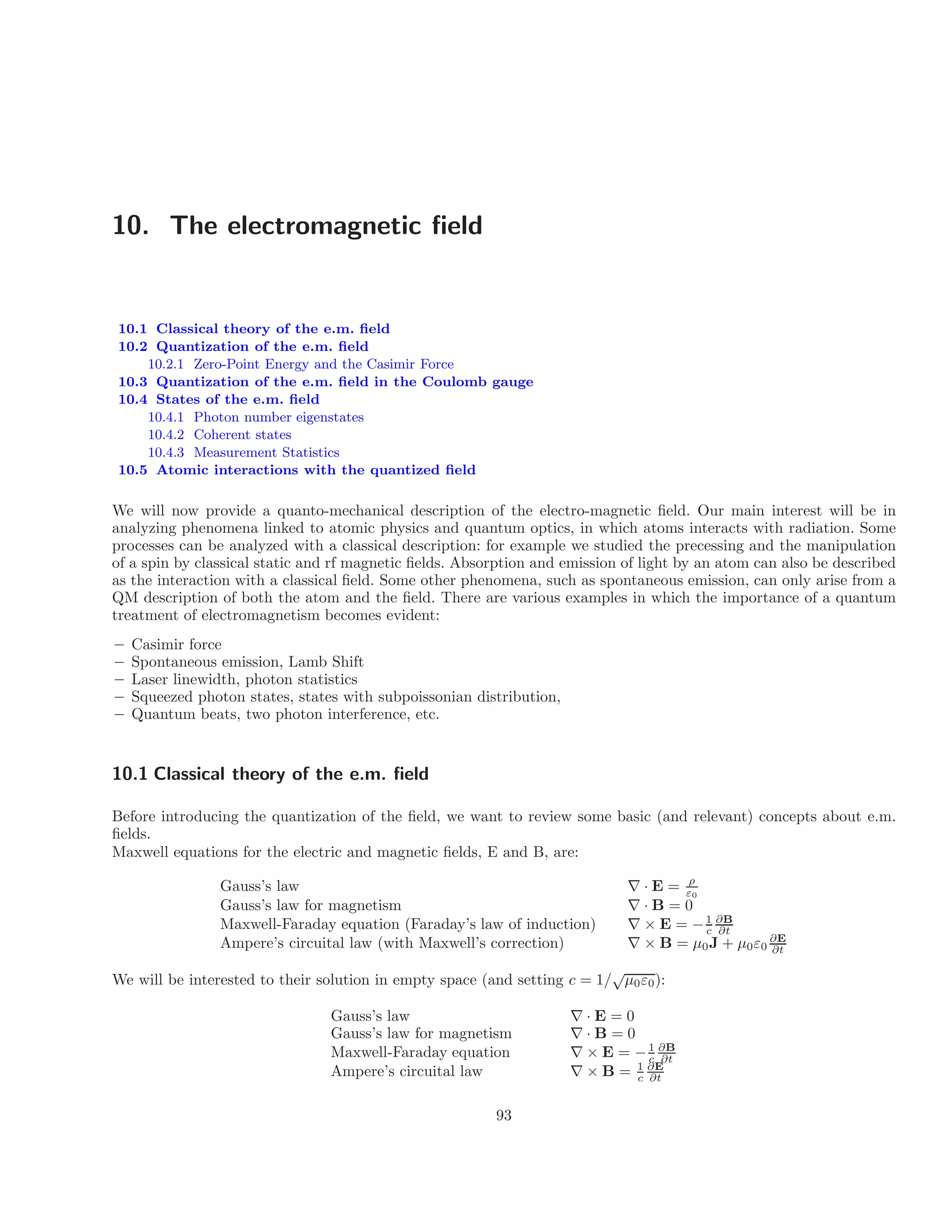
![Combining Maxwell equation in vacuum, we find the wave equations:
2 1 ∂2
E
∇ E − = 0 B
c2 t2
∇2 1 ∂2
B
∂
− = 0
c2 ∂t2
? Question: Show how this equation is derived
We need to take the curl of Maxwell-Faraday equation and the time derivative of Ampere’s law and use the vector identity
∇ × (∇ × ~
v) = ∇(∇ · ~
v) − ∇2
~
v and Gauss law.
~
A general solution for these equations can be written simply as E = E(ωt k ~
x). By fixing the boundary conditions,
we can find a solution in terms of an expansion in normal modes, where th
−
e tim
·
e dependence and spatial dependence
are separated. The solution of the wave equation can thus be facilitated by representing the electric field as a sum of
normal mode functions:
E(~
x, t) = fm(t)~
um(~
x).
m
The normal modes u are the equivalent of eigenfunc
X
m tions for the wave equation, so they do not evolve in time
(i.e. they are function of position only). The um are orthonormal functions, called normal modes. The boundary
conditions define the normal modes um for the field, satisfying:
∇2
um = −k2
mum, ∇ · um = 0, ~
n × um = 0
(where n is a unit vector normal to a surface). This last condition is imposed because the tangential component of
the electric field E must vanish on a conducting surface. We can also choose the modes to satisfy the orthonomality
condition (hence normal modes): Z
~
um(x)~
un(x)d3
x = δn,m
Substituting the expression for the electric field in the wave equation, we find an equation for the coefficient fm(t):
X d2
fm
+ c2
k2
mfm(t) = 0.
dt2
m
Since the mode functions are linearly independent, the coefficients of each mode must separately add up to zero in
order to satisfy the wave equation, and we find :
d2
fm
+ c2
k2
dt2 mfm(t) = 0.
As it can be seen from this equation, the dynamics of the normal modes, as described by their time-dependent
coefficients, is the same as that of the h.o. with frequency ωm = ckm. Hence the electric field is equivalent to an
infinite number of (independent) harmonic oscillators. In order to find a quantum-mechanical description of the e.m.
field we will need to turn this h.o. into quantum harmonic oscillators.
We want to express the magnetic field in terms of the same normal modes ~
um which are our basis. We assume for B
the expansion:
B(x, t) = hn(t) [
n
∇ × un(x)] ,
From Maxwell-Faraday law:
X
∇ × E =
X 1
fn(t)∇ × un = ∂
c
n
− tB
we see that we need to impose hn such that d hn
= −cfn so that we obtain
d t
X 1 d h
n
−
n 1
c d t
∇ × un = − ∂tB
c
94](https://image.slidesharecdn.com/theelectromagneticfield-210425174125/75/The-electromagnetic-field-2-2048.jpg)
![Notice that fn(t) is a function of time, so also the operators an(t) are (Heisenberg picture). The electric field is the
sum over this normal modes (notice that now the position is just a parameter, no longer an operator):
E(x, t) =
X p
2~πωn[a†
n(t) + an(t)]un(x)
n
Of course now the electric field is an operator field, that is, it is a QM operator that is defined at each space-time
point (x,t).
Notice that an equivalent formulation of the electric field in a finite volume V is given by defining in a slightly
different way the un(x) normal modes and writing:
E(x, t) =
X
r
2~πωn
[a†
n(t) + an(t)]un(x).
V
n
We already have calculated the evolution of the operator a and a†
. Each of the operator an evolves in the same way:
an(t) = an(0)e−iωnt
. This derives from the Heisenberg equation of motion dan
= i
~ [ , an(t)] = iωnan(t).
dt
The magnetic field can also be expressed in terms of the operators a
H −
n:
2π~
B(x, t) =
X
icn
r
[a†
n − an]
n
∇ )
ωn
× un(x
The strategy has been to use the known forms of the operators for a harmonic oscillator to deduce appropriate
dh (t)
operators for the e.m. field. Notice that we could have used the equation n
= cfn(t) to eliminate fn and write
dt
everything in terms of hn. This would have corresponded to identifying h
−
n with position and fn with momentum.
Since the Hamiltonian is totally symmetric in terms of momentum and position, the results are unchanged and we
can choose either formulations. In the case we chose, comparing the way in which the raising and lowering operators
enter in the E and B expressions with the way they enter the expressions for position and momentum, we may
say that, roughly speaking, the electric field is analogous to the position and the magnetic field is analogous to the
momentum of an oscillator.
10.2.1 Zero-Point Energy and the Casimir Force
The Hamiltonian operator for the e.m. field has the form of a harmonic oscillator for each mode of the field34
. As
we saw in a previous lecture, the lowest energy of a h.o. is 1
~ω. Since there are infinitely many modes of arbitrarily
2
high frequency in any finite volume, it follows that there should be an infinite zero-point energy in any volume of
space. Needless to say, this conclusion is unsatisfactory. In order to gain some appreciation for the magnitude of
the zero-point energy, we can calculate the zero-point energy in a rectangular cavity due to those field modes whose
frequency is less than some cutoff ωc. The mode functions un(x), solutions of the mode equation for a cavity of
dimensions Lx × Ly × Lz, have the vector components
un,α = Aα cos(kn,xrx) sin(kn,yry) sin(kn,zrz)
for {α, β, γ} = { ~
x, y, z} and permutations thereof. The mode un,α(x) are labeled by the wave-vector kn with compo-
nents: nαπ
kn,α = , nα
Lα
∈ N
and the frequency of the mode is ωn = k2 2
n,x + k2
n,y + kn,z. At least two of the integers must be nonzero, otherwise
the mode function would vanish identic
q
ally.
The amplitudes of the three components Aα are related by the divergence condition ∇ · ~
un(x) = 0, which requires
~ ~
that A · k = 0, from which it is clear that there are two linearly independent polarizations (directions of A) for each
34
See: Leslie E. Ballentine, “Quantum Mechanics A Modern Development”, World Scientific Publishing (1998). We follow
his presentation in this section.
96](https://image.slidesharecdn.com/theelectromagneticfield-210425174125/75/The-electromagnetic-field-4-2048.jpg)
![k, and hence there are two independent modes for each set of positive integers (nx, ny, nz). If one of the integers is
zero, two of the components of u(x) will vanish, so there is only one mode in this exceptional case.
In this case the electric field can be written as:
E(x, t) =
X
(Eα + Eα
†
) =
X
êα
X
r
~ωn ~ ~
[a†
ei(kn·~
r−ωt)
+ a ei(kn·~
r−ωt)
n ]
2ǫ0V n
α=1,2 α=1,2 n
Here V = LxLyLz is the volume of the cavity. Notice that the electric field associated with a single photon of
frequency ωn is
~ω
E
r
2π n
n =
V
This energy is a figure of merit for any phenomena relying on atomic interactions with a vacuum field, for example,
cavity quantum electrodynamics. In fact, En may be estimated by equating the quantum mechanical energy of a
photon ~ωn with its classical energy 1
dV (E2
+ B2
).
2
Going back to the calculation of the en
R
ergy density, if the dimensions of the cavity are large, the allowed values of k
approximate a continuum, and the density of modes in the positive octant of k space is ρ(k) = 2V/π3
(the factor 2
comes from the two possible polarizations). The zero-point energy density for all modes of frequency less that ωc is
then given by
k
2 c
1 2 1
E = ω ≈
Z
d3 1
~
0 k kρ(k) ~ω(k)
V 2 V 8 2
k=1
where we sum over all positive k (in the firs
X
t sum) and multiply by the number of possible polarizations (2). The
sum is then approximated by an integral over the positive octant (hence the 1/8 factor). Using ω(k) = kc (and
d3
k = 4πk2
dk), we obtain
2 2V 4π
E0 =
V π3 8
Z kc
1 kc
dk ~k3 c~ ~
c = dkk3 ck4
= c
2 2π2
k=0
Z
k=0 8π2
where we set the cutoff wave-vector kc = ωc/c. The factor k4
c indicates that this energy density is dominated by
the high-frequency, short-wavelength modes. Taking a minimum wavelength of λ 6
c = 2π/k = 0.4 10−
m, so as to
include the visible light spectrum, yields a zero-point energy density of 23 J/m3
. This may be com
×
pared with energy
density produced by a 100 W light bulb at a distance of 1 m, which is 2.7 10−8
J/m3
. Of course it is impossible
to extract any of the zero-point energy, since it is the minimum possible e
×
nergy of the field, and so our inability
to perceive that large energy density is not incompatible with its existence. Indeed, since most experiments detect
only energy differences, and not absolute energies, it is often suggested that the troublesome zero-point energy of
the field should simply be omitted. One might even think that this energy is only a constant background to every
experimental situation, and that, as such, it has no observable consequences. On the contrary, the vacuum energy
has direct measurable consequences, among which the Casimir effect is the most prominent one.
In 1948 H. B. G. Casimir showed that two electrically neutral, perfectly conducting plates, placed parallel in vacuum,
modify the vacuum energy density with respect to the unperturbed vacuum. The energy density varies with the
separation between the mirrors and thus constitutes a force between them, which scales with the inverse of the
forth power of the mirrors separation. The Casimir force is a small but well measurable quantity. It is a remarkable
macroscopic manifestation of a quantum effect and it gives the main contribution
bodies for distances beyond 100nm.
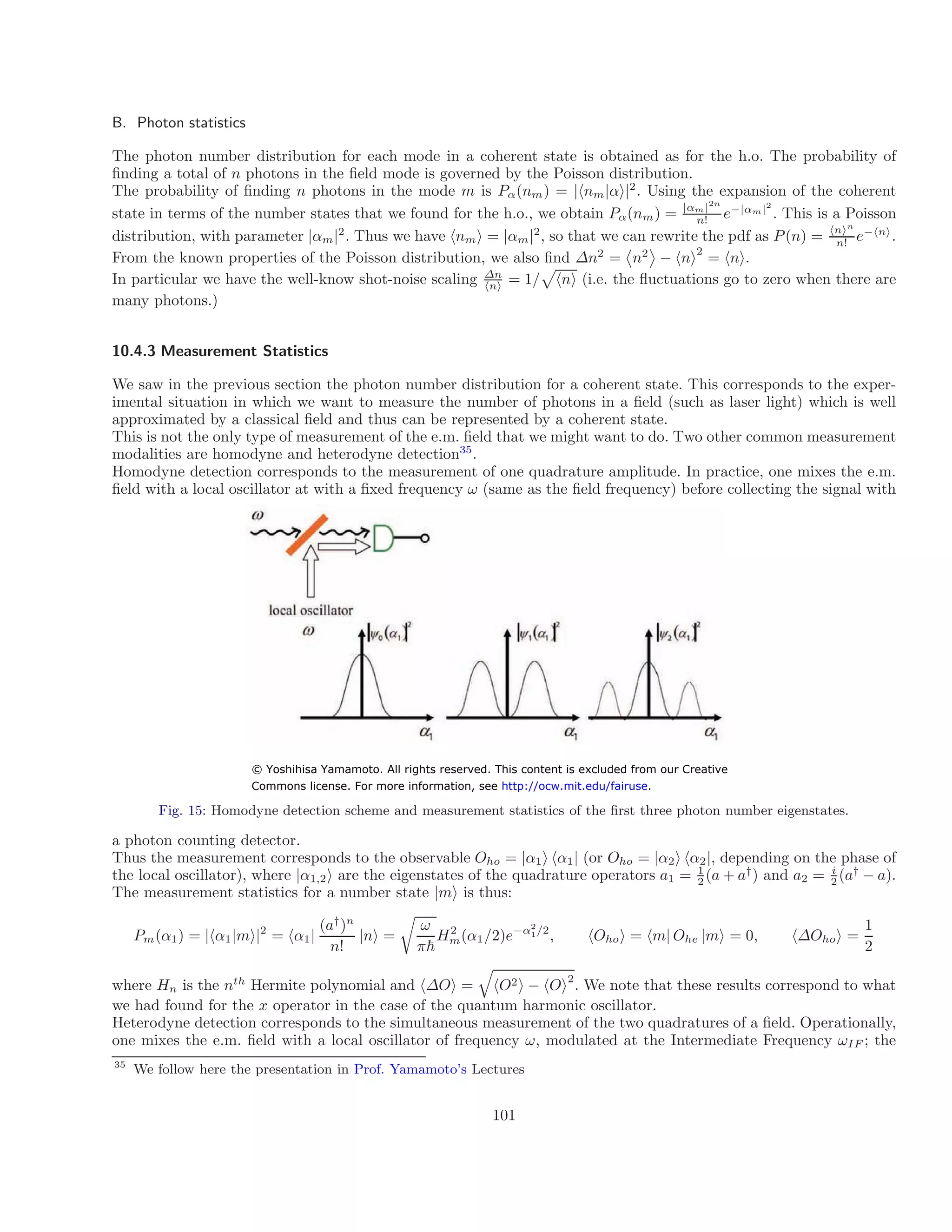
We consider a large cavity of dimensions V = L3
bounded by conducting walls
(see figure). A conducting plate is inserted at a distance R from one of the yz
faces (R ≪ L). The new boundary condition at x = R alters the energy (or
frequency) of each field mode. Following Casimir, we shall calculate the energy
shift as a function of R. Let WX denote the electromagnetic energy within a
cavity whose length in the x direction is X. The change in the energy due to the
insertion of the plate at x = R will be
∆W = (WR + WL R) W
− − L
Each of these three terms is infinite, but the difference will turn out to be finite.
Each mode has a zero-point energy of 1
~kc. But while we can take the continuous
2
97
to the forces between macroscopic
WL WR WL-R
L
R
Fig. 14: Geometry of Casimir Effect](https://image.slidesharecdn.com/theelectromagneticfield-210425174125/75/The-electromagnetic-field-5-2048.jpg)


![In a state with definite photon numbers, the electric and magnetic fields are indefinite and fluctuating. The probability
distributions for the electric and magnetic fields in such a state are analogous to the distributions for the position
and momentum of an oscillator in an energy eigenstate. Thus we have for the expectation value of the electric field
operator:
hE(x, t)i = h~
n| 2~πωm[a†
m(t) + am(t)]um(x)
m
|~
ni = 0
However, the second moment is non-zero:
X p
|E(x, t)|2
= 2π~
X √
ωpωm
[a†
p(t) + ap(t)][a†
m(t) + am(t)]
~
up(x) )
p
· ~
um(x
,m
= 2π~ ωm|um|2
[a†
m(t) + a ( 2
m t)]2
= 2π~ ωm um
m m
| (x)| (2nm + 1)
The sum over all modes is infin
X
ite. This div
ergence problem c
an often
X
be circumvented (but not solved) by recognizing
that a particular experiment will effectively couple to the EM field only over some finite bandwidth, thus we can set
cut-offs on the number of modes considered.
Notice that we can as well calculate ∆B for the magnetic field, to find the same expression.
10.4.2 Coherent states
A coherent state of the e.m. field is obtained by specifying a coherent state for each of the mode oscillators of the
field. Thus the coherent state vector will have the form
|α
~i = |α1α2 . . .i = |α1i ⊗ |α2i ⊗ . . .
It is parameterized by a denumberably infinite sequence of complex numbers. We now want to calculate the evolution
of the electric field for a coherent state. In the Heisenberg picture it is:
E(x, t) =
X p
2 t
~πω [a† m
meiω
m + a t
me−iωm
]um(x)
m
then, taking the expectation value we find:
hE(x, t)i =
X p
2~πωm[αm
∗
eiωmt
+ αme−iωmt
]um(x)
m
This is exactly the same form as a normal mode expansion of a classical solution of Maxwell’s equations, with the
parameter αm representing the amplitude of a classical field mode. In spite of this similarity, a coherent state of the
quantized EM field is not equivalent to a classical field, although it does give the closest possible quantum operator,
in terms of its expectation value. Even if the average field is equivalent to the classical field, there are still the
characteristic quantum fluctuations. A coherent state provides a good description of the e.m. field produced by a
laser. Most ordinary light sources emit states of the e.m. field that are very close to a coherent state (lasers), or to a
statistical mixture of coherent states (classical sources).
A. Fluctuations
We calculate the fluctuations for a single mode ∆Em. From
2
|Em
2
~
|2
= hαm| Em · Em |αmi we obtain ∆E2
m =
2π ωm|~
um(x)| . Indeed, from
(am + a†
m) we obtain:
hαm| (am
†
)2
+ a2
m + a†
mam + ama†
m |α
mi 2π~ω|um(x)|2
=
1 + ((α∗
m)2
+ α2
m + 2α∗
mαm)
2π~ω|um(x)|2
while we have
am + a†
m
= (αm + α∗
m)
√
2π~ωum(x), so that we obtain
(am + a†
m)2
−
am + a†
m
2
= 2π~ωm|~
um(x)|2
This is independent of αm, and is equal to the mean square fluctuation in the ground state. The Heisenberg inequality
is therefore saturated when the field is in a coherent state,
100](https://image.slidesharecdn.com/theelectromagneticfield-210425174125/75/The-electromagnetic-field-8-2048.jpg)

(where α is the polarization and m the mode). As in the semiclassical analysis, the Hamiltonian contains four terms,
which now have a clearer physical picture:
6 6
103](https://image.slidesharecdn.com/theelectromagneticfield-210425174125/75/The-electromagnetic-field-11-2048.jpg)


This document provides an introduction to quantizing the electromagnetic field. It begins with a classical description of the electromagnetic field using Maxwell's equations. It then shows that the classical electromagnetic field can be described as an infinite collection of independent harmonic oscillators. The document proceeds to quantize these harmonic oscillators by promoting the classical variables to quantum operators. This leads to a description of the electromagnetic field in terms of photon creation and annihilation operators. The quantized electromagnetic field gives rise to phenomena like zero-point energy and the Casimir effect that cannot be explained classically.


![Coded Agents – with UiPath SDK + LangGraph [Virtual Hands-on Workshop]](https://cdn.slidesharecdn.com/ss_thumbnails/codedagentsdeck-251215155422-5497c599-thumbnail.jpg?width=640&height=640&fit=bounds)


