This document contains lecture notes on quantum mechanics. It introduces key concepts like the Schrodinger equation, ket vectors, operators, and Hamiltonians. The notes are divided into multiple chapters that will cover topics such as the harmonic oscillator, angular momentum, perturbation theory, and other quantum systems. References are provided to textbooks where more of the material in the notes is based on. The notes are intended to review physical and mathematical concepts needed to formulate the theory of quantum mechanics.

![Preface
The dynamics of a quantum system is governed by the celebrated Schrödinger
equation
d
i |ψ = H |ψ , (0.1)
dt
√
where i = −1 and = 1.05457266 × 10⁻³⁴ J s is Planck’s h-bar constant.
However, what is the meaning of the symbols |ψ and H? The answers will
be given in the first part of the course (chapters 1-4), which reviews several
physical and mathematical concepts that are needed to formulate the theory
of quantum mechanics. We will learn that |ψ in Eq. (0.1) represents the
ket-vector state of the system and H represents the Hamiltonian operator.
The operator H is directly related to the Hamiltonian function in classical
physics, which will be defined in the first chapter. The ket-vector state and
its physical meaning will be introduced in the second chapter. Chapter 3
reviews the position and momentum operators, whereas chapter 4 discusses
dynamics of quantum systems. The second part of the course (chapters 5-7)
is devoted to some relatively simple quantum systems including a harmonic
oscillator, spin, hydrogen atom and more. In chapter 8 we will study quantum
systems in thermal equilibrium. The third part of the course (chapters 9-13)
is devoted to approximation methods such as perturbation theory, semiclas-
sical and adiabatic approximations. Light and its interaction with matter are
the subjects of chapter 14-15. Finally, systems of identical particles will be
discussed in chapter 16 and open quantum systems in chapter 17. Most of
the material in these lecture notes is based on the textbooks [1, 2, 3, 4, 6, 7].](https://image.slidesharecdn.com/qmlecturenotes-130118222159-phpapp01/85/Quantum-Mechanics-Lecture-notes-3-320.jpg)


![Chapter 2. State Vectors and Operators
While the multiplication of a bra-vector on the left and a ket-vector on the
right represents inner product, the outer product is obtained by reversing the
order
Aαβ = |α β| . (2.19)
The outer product Aαβ is clearly an operator since for any |γ ∈ F the object
Aαβ |γ is a ket-vector
Aαβ |γ = (|β α|) |γ = |β α |γ ∈ F . (2.20)
∈C
Moreover, according to property (2.4), Aαβ is linear since for every |γ 1 , |γ 2 ∈
F and c1 , c2 ∈ C the following holds
Aαβ (c1 |γ 1 + c2 |γ 2 ) = |α β| (c1 |γ 1 + c2 |γ 2 )
= |α (c1 β |γ 1 + c2 β |γ 2 )
= c1 Aαβ |γ 1 + c2 Aαβ |γ 2 .
(2.21)
With Dirac’s notation Eq. (2.10) can be rewritten as
|α = |φn φn | |α . (2.22)
n
Since the above identity holds for any |α ∈ F one concludes that the quantity
in brackets is the identity operator, which is denoted as 1, namely
1= |φn φn | . (2.23)
n
This result, which is called the closure relation, implies that any complete
orthonormal basis can be used to express the identity operator.
2.4 Dual Correspondence
As we have mentioned above, the bra-vector β| represents a functional map-
ping any ket-vector |α ∈ F to the complex number β |α . Moreover, since
the inner product is linear [see property (2.4) above], such a mapping is linear,
namely for every |γ 1 , |γ 2 ∈ F and c1 , c2 ∈ C the following holds
β| (c1 |γ 1 + c2 |γ 2 ) = c1 β |γ 1 + c2 β |γ 2 . (2.24)
The set of linear functionals from F to C, namely, the set of functionals F : F
→ C that satisfy
Eyal Buks Quantum Mechanics - Lecture Notes 18](https://image.slidesharecdn.com/qmlecturenotes-130118222159-phpapp01/85/Quantum-Mechanics-Lecture-notes-28-320.jpg)


![Chapter 2. State Vectors and Operators
complete. On the other hand, it can be shown that if a given Hermitian oper-
ator A satisfies some conditions (e.g., A needs to be completely continuous)
then completeness is guarantied. For all Hermitian operators of interest for
this course we will assume that all such conditions are satisfied. That is, for
any such Hermitian operator A there exists a set of ket vectors {|an,i }, such
that:
1. The set is orthonormal, namely
an′ ,i′ |an,i = δ nn′ δ ii′ , (2.64)
2. The ket-vectors |an,i are eigenvectors, namely
A |an,i = an |an,i , (2.65)
where an ∈ R.
3. The set is complete, namely closure relation [see also Eq. (2.23)] is satis-
fied
gn
1= |an,i an,i | = Pn , (2.66)
n i=1 n
where
gn
Pn = |an,i an,i | (2.67)
i=1
is the projector onto eigen subspace Fn with the corresponding eigenvalue
an .
The closure relation (2.66) can be used to express the operator A in terms
of the projectors Pn
gn gn
A = A1 = A |an,i an,i | = an |an,i an,i | , (2.68)
n i=1 n i=1
that is
A= an Pn . (2.69)
n
The last result is very useful when dealing with a function f (A) of the
operator A. The meaning of a function of an operator can be understood in
terms of the Taylor expansion of the function
f (x) = fm xm , (2.70)
m
Eyal Buks Quantum Mechanics - Lecture Notes 26](https://image.slidesharecdn.com/qmlecturenotes-130118222159-phpapp01/85/Quantum-Mechanics-Lecture-notes-36-320.jpg)


![Chapter 2. State Vectors and Operators
Tr (X) = an | X |an . (2.127)
n
It is easy to show that Tr (X) is independent on basis, as is shown below:
Tr (X) = an | X |an
n
= an |bk bk | X |bl bl |an
n,k,l
= bl |an an |bk bk | X |bl
n,k,l
= bl |bk bk | X |bl
k,l
δkl
= bk | X |bk .
k
(2.128)
The proof of the following relation
Tr (XY ) = Tr (Y X) , (2.129)
is left as an exercise.
2.11 Commutation Relation
The commutation relation of the operators A and B is defined as
[A, B] = AB − BA . (2.130)
As an example, the components Sx , Sy and Sz of the spin angular momentum
operator, satisfy the following commutation relations
[Si , Sj ] = i εijk Sk , (2.131)
where
0 i, j, k are not all different
εijk = 1 i, j, k is an even permutation of x, y, z (2.132)
−1 i, j, k is an odd permutation of x, y, z
is the Levi-Civita symbol. Equation (2.131) employs the Einstein’s conven-
tion, according to which if an index symbol appears twice in an expression,
it is to be summed over all its allowed values. Namely, the repeated index k
should be summed over the values x, y and z:
εijk Sk = εijx Sx + εijy Sy + εijz Sz . (2.133)
Eyal Buks Quantum Mechanics - Lecture Notes 34](https://image.slidesharecdn.com/qmlecturenotes-130118222159-phpapp01/85/Quantum-Mechanics-Lecture-notes-44-320.jpg)
![2.12. Simultaneous Diagonalization of Commuting Operators
Moreover, the following relations hold
2 2 2 1 2
Sx = Sy = Sz = , (2.134)
4
3 2
S2 = Sx + Sy + Sz =
2 2 2
. (2.135)
4
The relations below, which are easy to prove using the above definition,
are very useful for evaluating commutation relations
[F, G] = − [G, F ] , (2.136)
[F, F ] = 0 , (2.137)
[E + F, G] = [E, G] + [F, G] , (2.138)
[E, F G] = [E, F ] G + F [E, G] . (2.139)
2.12 Simultaneous Diagonalization of Commuting
Operators
Consider an observable A having a set of eigenvalues {an }. Let gn be the
degree of degeneracy of eigenvalue an , namely gn is the dimension of the
corresponding eigensubspace, which is denoted by Fn . Thus the following
holds
A |an,i = an |an,i , (2.140)
where i = 1, 2, · · · , gn , and
an′ ,i′ |an,i = δ nn′ δ ii′ . (2.141)
The set of vectors {|an,1 , |an,2 , · · · , |an,gn } forms an orthonormal basis for
the eigensubspace Fn . The closure relation can be written as
gn
1= |an,i an,i | = Pn , (2.142)
n i=1 n
where
gn
Pn = |an,i an,i | . (2.143)
i=1
Now consider another observable B, which is assumed to commute with
A, namely [A, B] = 0.
Claim. The operator B has a block diagonal matrix in the basis {|an,i },
namely am,j | B |an,i = 0 for n = m.
Eyal Buks Quantum Mechanics - Lecture Notes 35](https://image.slidesharecdn.com/qmlecturenotes-130118222159-phpapp01/85/Quantum-Mechanics-Lecture-notes-45-320.jpg)
![Chapter 2. State Vectors and Operators
Proof. Multiplying Eq. (2.140) from the left by am,j | B yields
am,j | BA |an,i = an am,j | B |an,i . (2.144)
On the other hand, since [A, B] = 0 one has
am,j | BA |an,i = am,j | AB |an,i = am am,j | B |an,i , (2.145)
thus
(an − am ) am,j | B |an,i = 0 . (2.146)
For a given n, the gn × gn matrix an,i′ | B |an,i is Hermitian, namely
∗
an,i′ | B |an,i = an,i | B |an,i′ . Thus, there exists a unitary transformation
Un , which maps Fn onto Fn , and which diagonalizes the block of B in the
subspace Fn . Since Fn is an eigensubspace of A, the block matrix of A in the
new basis remains diagonal (with the eigenvalue an ). Thus, we conclude that
a complete and orthonormal basis of common eigenvectors of both operators
A and B exists. For such a basis, which is denoted as {|n, m }, the following
holds
A |n, m = an |n, m , (2.147)
B |n, m = bm |n, m . (2.148)
2.13 Uncertainty Principle
Consider a quantum system in a state |n, m , which is a common eigenvector
of the commuting observables A and B. The outcome of a measurement of
the observable A is expected to be an with unity probability, and similarly,
the outcome of a measurement of the observable B is expected to be bm
with unity probability. In this case it is said that there is no uncertainty
corresponding to both of these measurements.
Definition 2.13.1. The variance in a measurement of a given observable A
of a quantum system in a state |α is given by (∆A)2 , where ∆A = A− A ,
namely
(∆A)2 = A2 − 2A A + A 2
= A2 − A 2
, (2.149)
where
A = α| A |α , (2.150)
A2 = α| A2 |α . (2.151)
Eyal Buks Quantum Mechanics - Lecture Notes 36](https://image.slidesharecdn.com/qmlecturenotes-130118222159-phpapp01/85/Quantum-Mechanics-Lecture-notes-46-320.jpg)
![2.13. Uncertainty Principle
Example 2.13.1. Consider a spin 1/2 system in a state |α = |+; ˆ . Using
z
Eqs. (2.99), (2.102) and (2.134) one finds that
(∆Sz )2 = Sz − Sz
2 2
=0, (2.152)
1
(∆Sx )2 = Sx − Sx
2 2
= 2
. (2.153)
4
The last example raises the question: can one find a state |α for which
the variance in the measurements of both Sz and Sx vanishes? According to
the uncertainty principle the answer is no.
Theorem 2.13.1. The uncertainty principle - Let A and B be two observ-
ables. For any ket-vector |α the following holds
2 1
(∆A) (∆B)2 ≥ | [A, B] |2 . (2.154)
4
Proof. Applying the Schwartz inequality [see Eq. (2.166)], which is given by
u |u v |v ≥ | u |v |2 , (2.155)
for the ket-vectors
|u = ∆A |α , (2.156)
|v = ∆B |α , (2.157)
and exploiting the fact that (∆A)† = ∆A and (∆B)† = ∆B yield
(∆A)2 (∆B)2 ≥ | ∆A∆B |2 . (2.158)
The term ∆A∆B can be written as
1 1
∆A∆B = [∆A, ∆B] + [∆A, ∆B]+ , (2.159)
2 2
where
[∆A, ∆B] = ∆A∆B − ∆B∆A , (2.160)
[∆A, ∆B]+ = ∆A∆B + ∆B∆A . (2.161)
While the term [∆A, ∆B] is anti-Hermitian, whereas the term [∆A, ∆B]+ is
Hermitian, namely
([∆A, ∆B])† = (∆A∆B − ∆B∆A)† = ∆B∆A − ∆A∆B = − [∆A, ∆B] ,
†
[∆A, ∆B]+ = (∆A∆B + ∆B∆A)† = ∆B∆A + ∆A∆B = [∆A, ∆B]+ .
In general, the following holds
∗ α| X |α ∗ if X is Hermitian
α| X |α = α| X † |α = , (2.162)
− α| X |α ∗ if X is anti-Hermitian
Eyal Buks Quantum Mechanics - Lecture Notes 37](https://image.slidesharecdn.com/qmlecturenotes-130118222159-phpapp01/85/Quantum-Mechanics-Lecture-notes-47-320.jpg)
![Chapter 2. State Vectors and Operators
thus
1 1
∆A∆B = [∆A, ∆B] + [∆A, ∆B]+ , (2.163)
2 2
∈I ∈R
and consequently
1 1 2
| ∆A∆B |2 = | [∆A, ∆B] |2 + [∆A, ∆B]+ . (2.164)
4 4
Finally, with the help of the identity [∆A, ∆B] = [A, B] one finds that
2 1
(∆A) (∆B)2 ≥ | [A, B] |2 . (2.165)
4
2.14 Problems
1. Derive the Schwartz inequality
| u |v | ≤ u |u v |v , (2.166)
where |u and |v are any two vectors of a vector space F.
2. Derive the triangle inequality:
( u| + v|) (|u + |v ) ≤ u |u + v |v . (2.167)
3. Show that if a unitary operator U can be written in the form U = 1+iǫF ,
where ǫ is a real infinitesimally small number, then the operator F is
Hermitian.
4. A Hermitian operator A is said to be positive-definite if, for any vector
|u , u| A |u ≥ 0. Show that the operator A = |a a| is Hermitian and
positive-definite.
5. Show that if A is a Hermitian positive-definite operator then the following
hold
| u| A |v | ≤ u| A |u v| A |v . (2.168)
6. Find the expansion of the operator (A − λB)−1 in a power series in λ ,
assuming that the inverse A−1 of A exists.
7. The derivative of an operator A (λ) which depends explicitly on a para-
meter λ is defined to be
dA (λ) A (λ + ǫ) − A (λ)
= lim . (2.169)
dλ ǫ→0 ǫ
Show that
d dA dB
(AB) = B+A . (2.170)
dλ dλ dλ
Eyal Buks Quantum Mechanics - Lecture Notes 38](https://image.slidesharecdn.com/qmlecturenotes-130118222159-phpapp01/85/Quantum-Mechanics-Lecture-notes-48-320.jpg)
![2.14. Problems
8. Show that
d dA −1
A−1 = −A−1 A . (2.171)
dλ dλ
9. Let |u and |v be two vectors of finite norm. Show that
Tr (|u v|) = v |u . (2.172)
10. If A is any linear operator, show that A† A is a positive-definite Her-
mitian operator whose trace is equal to the sum of the square moduli of
the matrix elements of A in any arbitrary representation. Deduce that
Tr A† A = 0 is true if and only if A = 0.
11. Show that if A and B are two positive-definite observables, then Tr (AB) ≥
0.
12. Show that for any two operators A and L
1 1
eL Ae−L = A + [L, A] + [L, [L, A]] + [L, [L, [L, A]]] + · · · . (2.173)
2! 3!
13. Show that if A and B are two operators satisfying the relation [[A, B] , A] =
0 , then the relation
[Am , B] = mAm−1 [A, B] (2.174)
holds for all positive integers m .
14. Show that
eA eB = eA+B e(1/2)[A,B] , (2.175)
provided that [[A, B] , A] = 0 and [[A, B] , B] = 0.
15. Proof Kondo’s identity
β
−βH −βH
A, e =e eλH [H, A] e−λH dλ , (2.176)
0
where A and H are any two operators and β is real.
16. Show that Tr (XY ) = Tr (Y X).
17. Consider the two normalized spin 1/2 states |α and |β . The operator
A is defined as
A = |α α| − |β β| . (2.177)
Find the eigenvalues of the operator A.
18. A molecule is composed of six identical atoms A1 , A2 , . . . , A6 which
form a regular hexagon. Consider an electron, which can be localized on
each of the atoms. Let |ϕn be the state in which it is localized on the
nth atom (n = 1, 2, · · · , 6). The electron states will be confined to the
Eyal Buks Quantum Mechanics - Lecture Notes 39](https://image.slidesharecdn.com/qmlecturenotes-130118222159-phpapp01/85/Quantum-Mechanics-Lecture-notes-49-320.jpg)


![2.15. Solutions
12. Let f (s) = esL Ae−sL , where s is real. Using Taylor expansion one has
1 df 1 d2 f
f (1) = f (0) + + +··· , (2.200)
1! ds s=0 2! ds2 s=0
thus
1 df 1 d2 f
eL Ae−L = A + + +··· , (2.201)
1! ds s=0 2! ds2 s=0
where
df
= LesL Ae−sL − esL Ae−sL L = [L, f (s)] , (2.202)
ds
d2 f df
2
= L, = [L, [L, f (s)]] , (2.203)
ds ds
therefore
1 1
eL Ae−L = A + [L, A] + [L, [L, A]] + [L, [L, [L, A]]] + · · · . (2.204)
2! 3!
13. The identity clearly holds for the case m = 1. Moreover, assuming it
holds for m, namely assuming that
[Am , B] = mAm−1 [A, B] , (2.205)
one has
Am+1 , B = A [Am , B] + [A, B] Am
= mAm [A, B] + [A, B] Am .
(2.206)
It is easy to show that if [[A, B] , A] = 0 then [[A, B] , Am ] = 0, thus one
concludes that
Am+1 , B = (m + 1) Am [A, B] . (2.207)
14. Define the function f (s) = esA esB , where s is real. The following holds
df
= AesA esB + esA BesB
ds
= A + esA Be−sA esA esB
Using Eq. (2.174) one has
Eyal Buks Quantum Mechanics - Lecture Notes 43](https://image.slidesharecdn.com/qmlecturenotes-130118222159-phpapp01/85/Quantum-Mechanics-Lecture-notes-53-320.jpg)
![Chapter 2. State Vectors and Operators
∞
sA (sA)m
e B= B
m=0
m!
∞
sm (BAm + [Am , B])
=
m=0
m!
∞
sm BAm + mAm−1 [A, B]
=
m=0
m!
∞ m−1
(sA)
= BesA + s [A, B]
m=1
(m − 1)!
= BesA + sesA [A, B] ,
(2.208)
thus
df
= AesA esB + BesA esB + sesA [A, B] esB
ds
= (A + B + [A, B] s) f (s) .
(2.209)
The above differential equation can be easily integrated since [[A, B] , A] =
0 and [[A, B] , B] = 0. Thus
s2
f (s) = e(A+B)s e[A,B] 2 . (2.210)
For s = 1 one gets
eA eB = eA+B e(1/2)[A,B] . (2.211)
15. Define
f (β) ≡ A, e−βH , (2.212)
β
−βH
g (β) ≡ e eλH [H, A] e−λH dλ . (2.213)
0
Clearly, f (0) = g (0) = 0 . Moreover, the following holds
df
= −AHe−βH + He−βH A = −Hf + [H, A] e−βH , (2.214)
dβ
dg
= −Hg + [H, A] e−βH , (2.215)
dβ
namely, both functions satisfy the same differential equation. Therefore
f = g.
16. Using a complete orthonormal basis {|n } one has
Eyal Buks Quantum Mechanics - Lecture Notes 44](https://image.slidesharecdn.com/qmlecturenotes-130118222159-phpapp01/85/Quantum-Mechanics-Lecture-notes-54-320.jpg)


![3. The Position and Momentum Observables
Consider a point particle moving in a 3 dimensional space. We first treat
the system classically. The position of the particle is described using the
Cartesian coordinates qx , qy and qz . Let
∂L
pj = (3.1)
∂ qj
˙
be the canonically conjugate variable to the coordinate qj , where j ∈ {x, y, z}
and where L is the Lagrangian. As we have seen in exercise 4 of set 1, the
following Poisson’s brackets relations hold
{qj , qk } = 0 , (3.2)
{pj , pk } = 0 , (3.3)
{qj , pk } = δ jk . (3.4)
In quantum mechanics, each of the 6 variables qx , qy , qz , px , py and pz is
represented by an Hermitian operator, namely by an observable. It is postu-
lated that the commutation relations between each pair of these observables
is related to the corresponding Poisson’s brackets according to the rule
1
{, } → [, ] . (3.5)
i
Namely the following is postulated to hold
[qj , qk ] = 0 , (3.6)
[pj , pk ] = 0 , (3.7)
[qj , pk ] = i δ jk . (3.8)
Note that here we use the same notation for a classical variable and its
quantum observable counterpart. In this chapter we will derive some results
that are solely based on Eqs. (3.6), (3.7) and (3.8).
3.1 The One Dimensional Case
In this section, which deals with the relatively simple case of a one dimen-
sional motion of a point particle, we employ the less cumbersome notation](https://image.slidesharecdn.com/qmlecturenotes-130118222159-phpapp01/85/Quantum-Mechanics-Lecture-notes-59-320.jpg)
![Chapter 3. The Position and Momentum Observables
x and p for the observables qx and px . The commutation relation between
these operators is given by [see Eq. (3.8)]
[x, p] = i . (3.9)
The uncertainty principle (2.154) employed for x and p yields
2
2
(∆x) (∆px )2 ≥ . (3.10)
4
3.1.1 Position Representation
Let x′ be an eigenvalue of the observable x, and let |x′ be the corresponding
eigenvector, namely
x |x′ = x′ |x′ . (3.11)
Note that x′ ∈ R since x is Hermitian. As we will see below transformation
between different eigenvectors |x′ can be performed using the translation
operator J (∆x ).
Definition 3.1.1. The translation operator is given by
i∆x p
J (∆x ) = exp − , (3.12)
where ∆x ∈ R.
Recall that in general the meaning of a function of an operator can be
understood in terms of the Taylor expansion of the function, that is, for the
present case
∞ n
1 i∆x p
J (∆x ) = − . (3.13)
n=0
n!
It is easy to show that J (∆x ) is unitary
J † (∆x ) = J (−∆x ) = J −1 (∆x ) . (3.14)
Moreover, the following composition property holds
J (∆x1 ) J (∆x2 ) = J (∆x1 + ∆x2 ) . (3.15)
Theorem 3.1.1. Let x′ be an eigenvalue of the observable x, and let |x′ be
the corresponding eigenvector. Then the ket-vector J (∆x ) |x′ is a normalized
eigenvector of x with an eigenvalue x′ + ∆x .
Eyal Buks Quantum Mechanics - Lecture Notes 50](https://image.slidesharecdn.com/qmlecturenotes-130118222159-phpapp01/85/Quantum-Mechanics-Lecture-notes-60-320.jpg)
![3.1. The One Dimensional Case
Proof. With the help of Eq. (3.77), which is given by
dB
[x, B (p)] = i , (3.16)
dp
and which is proven in exercise 1 of set 3, one finds that
∆x
[x, J (∆x )] = i J (∆x ) . (3.17)
i
Using this result one has
xJ (∆x ) |x′ = ([x, J (∆x )] + J (∆x ) x) |x′ = (x′ + ∆x ) J (∆x ) |x′ , (3.18)
thus the ket-vector J (∆x ) |x′ is an eigenvector of x with an eigenvalue x′ +
∆x . Moreover, J (∆x ) |x′ is normalized since J is unitary.
In view of the above theorem we will in what follows employ the notation
J (∆x ) |x′ = |x′ + ∆x . (3.19)
An important consequence of the last result is that the spectrum of eigenval-
ues of the operator x is continuous and contains all real numbers. This point
will be further discussed below.
The position wavefunction ψα (x′ ) of a state vector |α is defined as:
ψα (x′ ) = x′ |α . (3.20)
Given the wavefunction ψα (x′ ) of state vector |α , what is the wavefunction
of the state O |α , where O is an operator? We will answer this question below
for some cases:
1. The operator O = x. In this case
x′ | x |α = x′ x′ |α = x′ ψα (x′ ) , (3.21)
namely, the desired wavefunction is obtained by multiplying ψα (x′ ) by
x′ .
2. The operator O is a function A (x) of the operator x. Let
A (x) = an xn . (3.22)
n
be the Taylor expansion of A (x). Exploiting the fact that x is Hermitian
one finds that
x′ | A (x) |α = an x′ | xn |α = an x′n x′ |α = A (x′ ) ψα (x′ ) .
n n
x′n x′ |
(3.23)
Eyal Buks Quantum Mechanics - Lecture Notes 51](https://image.slidesharecdn.com/qmlecturenotes-130118222159-phpapp01/85/Quantum-Mechanics-Lecture-notes-61-320.jpg)


![Chapter 3. The Position and Momentum Observables
where ∆ = (∆x , ∆y , ∆z ) ∈ R3 , and where
J (∆) |r′ = |r′ + ∆ . (3.74)
The generalization of Eq. (3.52) for three dimensions is
1 ip′ · r′
r′ |p′ = exp . (3.75)
(2π )3/2
3.4 Problems
1. Show that
dA
[p, A (x)] = −i , (3.76)
dx
dB
[x, B (p)] = i , (3.77)
dp
where A (x) is a differentiable function of x and B (p) is a differentiable
function of p.
2. Show that the mean value of x in a state described by the wavefunction
ψ (x), namely
+∞
x = dxψ∗ (x) xψ (x) , (3.78)
−∞
is equal to the value of a for which the expression
+∞
F (a) ≡ dxψ∗ (x + a) x2 ψ (x + a) (3.79)
−∞
obtains a minimum, and that this minimum has the value
Fmin = (∆x)2 = x2 − x
2
. (3.80)
3. Consider a Gaussian wave packet, whose x space wavefunction is given
by
1 x′2
ψα (x′ ) = √ exp ikx′ − 2 . (3.81)
π1/4 d 2d
Calculate
a) (∆x)2 (∆p)2
b) p′ |α
Eyal Buks Quantum Mechanics - Lecture Notes 58](https://image.slidesharecdn.com/qmlecturenotes-130118222159-phpapp01/85/Quantum-Mechanics-Lecture-notes-68-320.jpg)
![3.4. Problems
4. Show that the state |α with wave function
√
1/ 2a for |x| ≤ a
x′ |α = (3.82)
0 for |x| > a
the uncertainty in momentum is infinity.
5. Show that
∞
d
p = −i dx′ |x′ x′ | . (3.83)
dx′
−∞
6. Show that
1 ip′ · (r′ − r′′ )
d3 p′ exp = δ (r′ − r′′ ) . (3.84)
(2π )3
7. Find eigenvectors and corresponding eigenvalues of the operator
O = p + Kx , (3.85)
where K is a real constant, p is the momentum operator, which is the
canonically conjugate to the position operator x. Calculate the wavefunc-
tion of the eigenvectors.
8. Let |α be the state vector of a point particle having mass m that moves
in one dimension along the x axis. The operator pα is defined by the
following requirements: (1) pα is Hermitian (i.e. p† = pα ) (2) [x, pα ] = 0
α
(i.e. pα commutes with the position operator x) and (3)
α| (p − pα )2 |α = min α| (p − O)2 |α , (3.86)
O
where p is the momentum operator (i.e. the minimum value of the quan-
tity α| (p − O)2 |α is obtained when the operator O is chosen to be
pα ).
a) Calculate the matrix elements x′ | pα |x′′ of the operator pα in the
position representation.
b) The operator P is the difference between the ’true’ momentum op-
erator and pα
P = p − pα . (3.87)
Calculate the variance (∆P)2 with respect to the state |α
(∆P)2 = α| P 2 |α − α| P |α
2
. (3.88)
Eyal Buks Quantum Mechanics - Lecture Notes 59](https://image.slidesharecdn.com/qmlecturenotes-130118222159-phpapp01/85/Quantum-Mechanics-Lecture-notes-69-320.jpg)
![Chapter 3. The Position and Momentum Observables
c) Use your results to prove the uncertainty relation (3.10)
2
(∆x)2 (∆p)2 ≥ . (3.89)
4
where
(∆x)2 = α| x2 |α − α| x |α 2
, (3.90)
and where
(∆p)2 = α| p2 |α − α| p |α 2
. (3.91)
3.5 Solutions
1. The commutator [x, p] = i is a constant, thus the relation (2.174) can
be employed
dxm
[p, xm ] = −i mxm−1 = −i , (3.92)
dx
m
dp
[x, pm ] = i mpm−1 = i . (3.93)
dp
This holds for any m, thus, for any differentiable function A (x) of x and
for any differentiable function B (p) of p one has
dA
[p, A (x)] = −i , (3.94)
dx
dB
[x, B (p)] = i . (3.95)
dp
2. The following holds
+∞
F (a) = dxψ∗ (x + a) x2 ψ (x + a)
−∞
+∞
2
= dx′ ψ∗ (x′ ) (x′ − a) ψ (x′)
−∞
= (x − a)2
= x2 − 2a x + a2 .
(3.96)
The requirement
dF
=0 (3.97)
da
Eyal Buks Quantum Mechanics - Lecture Notes 60](https://image.slidesharecdn.com/qmlecturenotes-130118222159-phpapp01/85/Quantum-Mechanics-Lecture-notes-70-320.jpg)

![3.5. Solutions
5. Using Eqs. (3.29) and (3.32) one has
∞
p |α = dx′ |x′ x′ | p |α
−∞
∞
d
= −i dx′ |x′ x′ |α ,
dx′
−∞
(3.106)
thus, since |α is an arbitrary ket vector, the following holds
∞
d
p = −i dx′ |x′ x′ | . (3.107)
dx′
−∞
6. With the help of Eqs. (3.66), (3.71) and (3.75) one finds that
δ (r′ − r′′ ) = r′ |r′′
= d3 p′ r′ |p′ p′ |r′′
1 ip′ · (r′ − r′′ )
= d3 p′ exp .
(2π )3
(3.108)
7. Using the identity (2.173), which is given by
1 1
eL Ae−L = A + [L, A] + [L, [L, A]] + [L, [L, [L, A]]] + · · · . (3.109)
2! 3!
and the identity (3.76), which is given by
dg
[g (x) , p] = i , (3.110)
dx
one finds that
dg i dg i dg
eg(x) pe−g(x) = A+i + g (x) , + g (x) , g (x) , +· · · .
dx 2! dx 3! dx
(3.111)
Choosing g (x) to be given by
Kx2
g (x) = (3.112)
2i
yields
UpU † = A + Kx = O , (3.113)
Eyal Buks Quantum Mechanics - Lecture Notes 63](https://image.slidesharecdn.com/qmlecturenotes-130118222159-phpapp01/85/Quantum-Mechanics-Lecture-notes-73-320.jpg)
![Chapter 3. The Position and Momentum Observables
where the unitary operator U is given by
iKx2
U = e− 2 .
Thus, the vectors |ψ (p′ ) , which are define as
|ψ (p′ ) = U |p′ , (3.114)
where |p′ is an eigenvector of p with eigenvalue p′ (i.e. p |p′ = p′ |p′ ),
are eigenvectors of O, and the following holds
O |ψ (p′ ) = p′ |ψ (p′ ) . (3.115)
With the help of Eq. (3.52), which is given by
1 ip′ x′
x′ |p′ = √ e , (3.116)
2π
one finds that the wavefunction ψ (x′ ; p′ ) = x′ |ψ (p′ ) of the state
|ψ (p′ ) is given by
iKx′2
ψ (x′ ; p′ ) = e− 2 x′ |p′
1 i ′2
p′ x′ − Kx
= √ e 2
.
2π
(3.117)
8. With the help of Eq. (3.32) one finds that
∞ ∞
pα = dx′ dx′′ |x′ x′ | pα |x′′ x′′ | . (3.118)
−∞ −∞
The requirement [x, pα ] = 0 implies that
∞ ∞
′
dx dx′′ |x′ x′ | pα |x′′ (x′ − x′′ ) x′′ | = 0 , (3.119)
−∞ −∞
hence x′ | pα |x′′ = 0 unless x′ = x′′ . Thus by using the notation
x′ | pα |x′′ = φα (x′ ) δ (x′ − x′′ ) , (3.120)
the operator pα can be expressed as
∞
pα = dx′ |x′ φα (x′ ) x′ | . (3.121)
−∞
The requirement that pα is Hermitian implies that φα (x′ ) is real.
Eyal Buks Quantum Mechanics - Lecture Notes 64](https://image.slidesharecdn.com/qmlecturenotes-130118222159-phpapp01/85/Quantum-Mechanics-Lecture-notes-74-320.jpg)
![Chapter 3. The Position and Momentum Observables
d log ψα
ψ∗
x′ | pα |x′′ = α
δ (x′ − x′′ ) . (3.129)
2i dx′
Note: Comparing this result with the expression for the current den-
sity J associated with the state |α [see Eq. (4.174)] yields the fol-
lowing relation
dψα
J= Im ψ∗ α
m dx′
′
ρ (x ) d logψα d logψ∗ α
= −
m 2i dx′ dx′
ρ (x′ )
= φ (x′ ) .
m α
(3.130)
b) As can be seen from Eqs. (3.123) and (3.128) the following holds
∞
ψα
d 1 d log ψ∗ ′
P =i dx′ |x′ − ′ + α
x| , (3.131)
dx 2 dx′
−∞
hence ∞
dψα 1 dψα dψ∗
α| P |α = i dx′ −ψ∗
α + ψ∗
α − α
ψ
dx′ 2 dx′ dx′ α
−∞
∞
i dψα dψ∗
=− dx′ ψ∗
α + α
ψ
2 dx′ dx′ α
−∞
∞
i dρ (x′ )
=− dx′
2 dx′
−∞
=0,
(3.132)
thus [see Eqs. (3.126) and (3.128)]
(∆P)2 = α| P 2 |α
∞
2 2
d logψα d logψ∗α
= dx′ ρ (x′ ) +
2 dx′ dx′
−∞
∞
2 2
d logρ (x′ )
= dx′ ρ (x′ ) .
2 dx′
−∞
(3.133)
Note that the result α| P |α = 0 implies that pα and p have the
same expectation value, i.e. α| pα |α = α| p |α . On the other hand,
Eyal Buks Quantum Mechanics - Lecture Notes 66](https://image.slidesharecdn.com/qmlecturenotes-130118222159-phpapp01/85/Quantum-Mechanics-Lecture-notes-76-320.jpg)
![Chapter 3. The Position and Momentum Observables
is the expectation value of x, yields
2
∞
′ ′ ′ d logρ(x′ )
∞
2
dx ρ (x ) (x − x ) dx′
′ ′ d logρ (x′ ) −∞
dx ρ (x ) ≥ ,
dx′ (∆x)2
−∞
(3.141)
where
∞
2 2
(∆x) = dx′ ρ (x′ ) (x′ − x ) (3.142)
−∞
is the variance of x. By integrating by parts one finds that
∞ ∞
′ ′ d logρ (x′ )
′ dρ (x′ )
dx ρ (x ) (x − x ) = dx′ (x′ − x )
dx′ dx′
−∞ −∞
∞
=− dx′ ρ (x′ )
−∞
= −1 .
(3.143)
Combining these results [see Eqs. (3.137) and (3.141)] lead to
2
(∆x)2 (∆p)2 ≥ . (3.144)
2
Eyal Buks Quantum Mechanics - Lecture Notes 68](https://image.slidesharecdn.com/qmlecturenotes-130118222159-phpapp01/85/Quantum-Mechanics-Lecture-notes-78-320.jpg)
![4.3. Example - Spin 1/2
and Eq. (4.9) one finds that
iH (t − t0 )
u (t, t0 ) = exp − 1
gn
iH (t − t0 )
= exp − |an,i an,i |
n i=1
gn
iEn (t − t0 )
= exp − |an,i an,i | .
n i=1
(4.13)
Using this results the state vector |α (t) can be written as
|α (t) = u (t, t0 ) |α (t0 )
gn
iEn (t − t0 )
= exp − an,i |α (t0 ) |an,i .
n i=1
(4.14)
Note that if the system is initially in an eigenvector of the Hamiltonian
with eigenenergy En , then according to Eq. (4.14)
iEn (t − t0 )
|α (t) = exp − |α (t0 ) . (4.15)
However, the phase factor multiplying |α (t0 ) has no effect on any mea-
surable physical quantity of the system, that is, the system’s properties are
time independent. This is why the eigenvectors of the Hamiltonian are called
stationary states.
4.3 Example - Spin 1/2
In classical mechanics, the potential energy U of a magnetic moment µ in a
magnetic field B is given by
U = −µ · B . (4.16)
The magnetic moment of a spin 1/2 is given by [see Eq. (2.90)]
2µB
µspin = S, (4.17)
where S is the spin angular momentum vector and where
e
µB = (4.18)
2me c
Eyal Buks Quantum Mechanics - Lecture Notes 71](https://image.slidesharecdn.com/qmlecturenotes-130118222159-phpapp01/85/Quantum-Mechanics-Lecture-notes-81-320.jpg)
![Chapter 4. Quantum Dynamics
is the Bohr’s magneton (note that the electron charge is taken to be negative
e < 0). Based on these relations we hypothesize that the Hamiltonian of a
spin 1/2 in a magnetic field B is given by
e
H=− S·B. (4.19)
me c
Assume the case where
B = Bˆ ,
z (4.20)
where B is a constant. For this case the Hamiltonian is given by
H = ωSz , (4.21)
where
|e| B
ω= (4.22)
me c
is the so-called Larmor frequency. In terms of the eigenvectors of the operator
Sz
Sz |± = ± |± , (4.23)
2
where the compact notation |± stands for the states |±; ˆ , one has
z
ω
H |± = ± |± , (4.24)
2
namely the states |± are eigenstates of the Hamiltonian. Equation (4.13) for
the present case reads
iωt iωt
u (t, 0) = e− 2 |+ +| + e 2 |− −| . (4.25)
Exercise 4.3.1. Consider spin 1/2 in magnetic field given by B = Bˆ, where
z
B is a constant. Given that |α (0) = |+; x at time t = 0 calculate (a) the
ˆ
probability p± (t) to measure Sx = ± /2 at time t; (b) the expectation value
Sx (t) at time t.
Solution 4.3.1. Recall that [see Eq. (2.102)]
1
|±; x = √ (|+ ± |− )
ˆ (4.26)
2
(a) Using Eq. (4.25) one finds
p± (t) = | ±; x| u (t, 0) |α (0) |2
ˆ
2
1 iωt iωt
= ( +| ± −|) e− 2 |+ +| + e 2 |− −| (|+ + |− )
2
2
1 − iωt iωt
= e 2 ±e 2 ,
2
(4.27)
Eyal Buks Quantum Mechanics - Lecture Notes 72](https://image.slidesharecdn.com/qmlecturenotes-130118222159-phpapp01/85/Quantum-Mechanics-Lecture-notes-82-320.jpg)

![Chapter 4. Quantum Dynamics
dA(H) du† du ∂A
= Au + u† A + u† u
dt dt dt ∂t
1 ∂A
= −u† HAu + u† AHu + u† u
i ∂t
1 ∂A
= −u† Huu† Au + u† Auu† Hu + u† u
i ∂t
1 ∂A(H)
= −H(H) A(H) + A(H) H(H) + .
i ∂t
(4.36)
Thus, we have found that
dA(H) 1 ∂A(H)
= A(H) , H(H) + . (4.37)
dt i ∂t
Furthermore, the desired equation of motion for A is found using Eqs. (4.32)
and (4.37)
d A 1 ∂A
= [A, H] + . (4.38)
dt i ∂t
We see that the Poisson’s brackets in the classical equation of motion (4.31)
for the classical variable A(c) are replaced by a commutation relation in the
quantum counterpart equation of motion (4.38) for the expectation value A
1
{, } → [, ] . (4.39)
i
Note that for the case where the Hamiltonian is time independent, namely
for the case where the time evolution operator is given by Eq. (4.9), u com-
mutes with H, namely [u, H] = 0, and consequently
H(H) = u† Hu = H . (4.40)
4.5 Symmetric Ordering
What is in general the correspondence between a classical variable and its
quantum operator counterpart? Consider for example the system of a point
particle moving in one dimension. Let x(c) be the classical coordinate and let
p(c) be the canonically conjugate momentum. As we have done in chapter 3,
the quantum observables corresponding to x(c) and p(c) are the Hermitian
operators x and p. The commutation relation [x, p] is derived from the cor-
responding Poisson’s brackets x(c) , p(c) according to the rule
1
{, } → [, ] , (4.41)
i
Eyal Buks Quantum Mechanics - Lecture Notes 74](https://image.slidesharecdn.com/qmlecturenotes-130118222159-phpapp01/85/Quantum-Mechanics-Lecture-notes-84-320.jpg)
![4.5. Symmetric Ordering
namely
x(c) , p(c) = 1 → [x, p] = i . (4.42)
However, what is the quantum operator corresponding to a general func-
tion A x(c) , p(c) of x(c) and p(c) ? This question raises the issue of order-
ing. As an example, let A x(c) , p(c) = x(c) p(c) . Classical variables obviously
commute, therefore x(c) p(c) = p(c) x(c) . However, this is not true for quantum
operators xp = px. Moreover, it is clear that both operators xp and px cannot
be considered as observables since they are not Hermitian
(xp)† = px = xp , (4.43)
†
(px) = xp = px . (4.44)
A better candidate to serve as the quantum operator corresponding to the
classical variables x(c) p(c) is the operator (xp + px) /2, which is obtained from
x(c) p(c) by a procedure called symmetric ordering. A general transformation
that produces a symmetric ordered observable A (x, p) that corresponds to
a given general function A x(c) , p(c) of the classical variable x(c) and its
canonical conjugate p(c) is given below
∞ ∞
A (x, p) = A x(c) , p(c) Υ dx(c) dp(c) ,
−∞ −∞
(4.45)
where
∞ ∞
1 (c) (c)
e (η(x −x)+ξ(p −p)) dηdξ .
i
Υ = 2 (4.46)
(2π )
−∞ −∞
This transformation is called the Weyl transformation. The identity
∞
′ ′′
dkeik(x −x ) = 2πδ (x′ − x′′ ) , (4.47)
−∞
implies that
1 i
η(x(c) −x)
e dη = δ x(c) − x , (4.48)
2π
1 i
ξ(p(c) −p)
e dξ = δ p(c) − p . (4.49)
2π
At first glance these relations may lead to the (wrong) conclusion that the
term Υ equals to δ x(c) − x δ p(c) − p , however, this is incorrect since x
and p are non-commuting operators.
Eyal Buks Quantum Mechanics - Lecture Notes 75](https://image.slidesharecdn.com/qmlecturenotes-130118222159-phpapp01/85/Quantum-Mechanics-Lecture-notes-85-320.jpg)
![4.6. Problems
6. Show that if the potential energy V (r) can be written as a sum of func-
tions of a single coordinate, V (r) = V1 (x1 ) + V2 (x2 ) + V3 (x3 ), then the
time-independent Schrödinger equation can be decomposed into a set of
one-dimensional equations of the form
d2 ψi (xi ) 2m
+ 2 [Ei − Vi (xi )] ψi (xi ) = 0 , (4.58)
dx2i
where i ∈ {1, 2, 3}, with ψ (r) = ψ1 (x1 ) ψ2 (x2 ) ψ3 (x3 ) and E = E1 +
E2 + E3 .
7. Show that, in one-dimensional problems, the energy spectrum of the
bound states is always non-degenerate.
8. Let ψn (x) (n = 1, 2, 3, · · · ) be the eigen-wave-functions of a one-
dimensional Schrödinger equation with eigen-energies En placed in order
of increasing magnitude (E1 < E2 < · · · . ). Show that between any two
consecutive zeros of ψn (x), ψn+1 (x) has at least one zero.
9. What conclusions can be drawn about the parity of the eigen-functions
of the one-dimensional Schrödinger equation
d2 ψ (x) 2m
+ 2 (E − V (x)) ψ (x) = 0 (4.59)
dx2
if the potential energy is an even function of x , namely V (x) = V (−x).
10. Show that the first derivative of the time-independent wavefunction is
continuous even at points where V (x) has a finite discontinuity.
11. A particle having mass m is confined by a one dimensional potential given
by
−W if |x| ≤ a
Vs (x) = , (4.60)
0 if |x| > a
where a > 0 and W > 0 are real constants. Show that the particle has
at least one bound state (i.e., a state having energy E < 0 ).
12. Consider a particle having mass m confined in a potential well given by
0 if 0 ≤ x ≤ a
V (x) = . (4.61)
∞ if x < 0 or x > a
The eigen energies are denoted by En and the corresponding eigen states
are denoted by |ϕn , where n = 1, 2, · · · (as usual, the states are num-
bered in increasing order with respect to energy). The state of the system
at time t = 0 is given by
|Ψ (0) = a1 |ϕ1 + a2 |ϕ2 + a3 |ϕ3 . (4.62)
(a) The energy E of the system is measured at time t = 0 . What is the
probability to measure a value smaller than 3π 2 2 / ma2 ? (b) Calculate
Eyal Buks Quantum Mechanics - Lecture Notes 77](https://image.slidesharecdn.com/qmlecturenotes-130118222159-phpapp01/85/Quantum-Mechanics-Lecture-notes-87-320.jpg)
![Chapter 4. Quantum Dynamics
d Sx ω
= [Sx , Sz ] = −ω Sy , (4.72)
dt i
d Sy ω
= [Sy , Sz ] = ω Sx , (4.73)
dt i
d Sz ω
= [Sz , Sz ] = 0 , (4.74)
dt i
where
|e| B
ω= . (4.75)
me c
At time t = 0 the system is in state
1
|+; x = √ (|+ + |− ) ,
ˆ (4.76)
2
thus
Sx (t = 0) = ( +| + −|) (|+ −| + |− +|) (|+ + |− ) = .
4 2
Sy (t = 0) = ( +| + −|) (−i |+ −| + i |− +|) (|+ + |− ) = 0 .
4
Sz (t = 0) = ( +| + −|) (|+ +| − |− −|) (|+ + |− ) = 0 .
4
The solution is easily found to be given by
Sx (t) = cos (ωt) , (4.77)
2
Sy (t) = sin (ωt) , (4.78)
2
Sz (t) = 0 . (4.79)
2. The Hamiltonian operator H is given by
p2
H= + V (x) . (4.80)
2m
Multiplying the relation
H |ψn = En |ψn (4.81)
from the left by x′ | yields [see Eqs. (3.23) and (3.29)]
2
d2 ψn (x′ )
− + V (x′ ) ψ n (x′ ) = En ψn (x′ ) , (4.82)
2m dx′2
where
ψn (x′ ) = x′ |ψn (4.83)
is the wavefunction in the coordinate representation.
Eyal Buks Quantum Mechanics - Lecture Notes 80](https://image.slidesharecdn.com/qmlecturenotes-130118222159-phpapp01/85/Quantum-Mechanics-Lecture-notes-90-320.jpg)
![4.7. Solutions
3. Using [x, px ] = [y, py ] = [z, pz ] = i one finds that
p2
[H, r] = ,r
2m
1
= p2 , x , p2 , y , p2 , z
x y z
2m
= (px , py , pz )
im
= p.
im
(4.84)
Thus
im
ψn | p |ψn = ψn | [H, r] |ψn
im
= ψn | (Hr − rH) |ψn
imEn
= ψn | (r − r) |ψn
=0.
(4.85)
4. Multiplying Eq. (4.53) from the left by the bra p′ | and inserting the
closure relation
1= dp′′ |p′′ p′′ | (4.86)
yields
dφα (p′ )
i = dp′′ p′ | H |p′′ φα (p′′ ) . (4.87)
dt
The following hold
p′ | p2 |p′′ = p′2 δ (p′ − p′′ ) , (4.88)
and
p′ | V (r) |p′′ = dr′ dr′′ p′ |r′ r′ | V (r) |r′′ r′′ |p′′
ip′ · r′ ip′′ · r′′
= (2π )−3 dr′ dr′′ exp − V (r′ ) δ (r′ − r′′ ) exp
i (p′ − p′′ ) · r′
= (2π )−3 dr′ exp − V (r′ )
= U (p′ − p′′ ) ,
(4.89)
Eyal Buks Quantum Mechanics - Lecture Notes 81](https://image.slidesharecdn.com/qmlecturenotes-130118222159-phpapp01/85/Quantum-Mechanics-Lecture-notes-91-320.jpg)
![Chapter 4. Quantum Dynamics
thus the momentum wave functionφα (p′ ) satisfies the following equation
dφα p′2
i = φ + dp′′ U (p′ − p′′ ) φα . (4.90)
dt 2m α
5. The Hamiltonian is given by
p2
H= + V (r) . (4.91)
2m
Using Eq. (4.38) one has
d x 1 1 px
= [x, H] = x, p2
x = , (4.92)
dt i i 2m m
and
d px 1
= [px , V (r)] , (4.93)
dt i
or with the help of Eq. (3.76)
d px ∂V
=− . (4.94)
dt ∂x
This together with Eq. (4.92) yield
d2 x ∂V
m =− . (4.95)
dt2 ∂x
Similar equations are obtained for y and z , which together yield Eq.
(4.57).
6. Substituting a solution having the form
ψ (r) = ψ1 (x1 ) ψ2 (x2 ) ψ3 (x3 ) (4.96)
into the time-independent Schrödinger equation, which is given by
2m
∇2 ψ (r) + 2
[E − V (r)] ψ (r) = 0 , (4.97)
and dividing by ψ (r) yield
3
1 d2 ψi (xi ) 2m 2m
− 2 Vi (xi ) =− E. (4.98)
i=1
ψi (xi ) dx2
i
2
In the sum, the ith term (i ∈ {1, 2, 3}) depends only on xi , thus each
term must be a constant
1 d2 ψi (xi ) 2m 2m
2 − 2 Vi (xi ) = − 2 Ei , (4.99)
ψ i (xi ) dxi
where E1 + E2 + E3 = E.
Eyal Buks Quantum Mechanics - Lecture Notes 82](https://image.slidesharecdn.com/qmlecturenotes-130118222159-phpapp01/85/Quantum-Mechanics-Lecture-notes-92-320.jpg)
![Chapter 4. Quantum Dynamics
with the same E. Therefore, all eigen-wave-functions can be chosen to be
real (i.e., by the transformation ψ (x) → (ψ (x) + ψ∗ (x)) /2). We have
d2 ψn 2m
+ 2 (En − V (x)) ψn = 0 , (4.110)
dx2
d2 ψn+1 2m
+ 2 (En+1 − V (x)) ψn+1 = 0 . (4.111)
dx2
By multiplying the first Eq. by ψn+1 , the second one by ψn , and sub-
tracting one has
d2 ψn d2 ψn+1 2m
ψn+1 − ψn + 2 (En − En+1 ) ψn ψ n+1 = 0 , (4.112)
dx2 dx2
or
d dψn dψ 2m
ψn+1 − ψn n+1 + 2
[En − En+1 ] ψn ψn+1 = 0 . (4.113)
dx dx dx
Let x1 and x2 be two consecutive zeros of ψn (x) (i.e., ψn (x1 ) =
ψn (x2 ) = 0). Integrating from x1 to x2 yields
x2
x2
dψn+1
ψn+1 dψn − ψn =
2m
(En+1 − En ) dxψ n ψn+1 .
dx dx 2
x1
=0 x1 >0
(4.114)
Without lost of generality, assume that ψn (x) > 0 in the range (x1 , x2 ).
Since ψn (x) is expected to be continuous, the following must hold
dψn
>0, (4.115)
dx x=x1
dψn
<0. (4.116)
dx x=x2
As can be clearly seen from Eq. (4.114), the assumption that ψn+1 (x) > 0
in the entire range (x1 , x2 ) leads to contradiction. Similarly, the possibil-
ity that ψn+1 (x) < 0 in the entire range (x1 , x2 ) is excluded. Therefore,
ψn+1 must have at least one zero in this range.
9. Clearly if ψ (x) is an eigen function with energy E, also ψ (−x) is an
eigen function with the same energy. Consider two cases: (i) The level E
is non-degenerate. In this case ψ (x) = cψ (−x), where c is a constant.
Normalization requires that |c|2 = 1. Moreover, since the wavefunctions
can be chosen to be real, the following holds: ψ (x) = ±ψ (−x). (ii) The
level E is degenerate. In this case every superposition of ψ (x) and ψ (−x)
can be written as a superposition of an odd eigen function ψodd (x) and
an even one ψ even (x), which are defined by
Eyal Buks Quantum Mechanics - Lecture Notes 84](https://image.slidesharecdn.com/qmlecturenotes-130118222159-phpapp01/85/Quantum-Mechanics-Lecture-notes-94-320.jpg)


![Chapter 4. Quantum Dynamics
a 2
∆x 2 nπ
pn = dxψ∗ (x) ψ (x)
n ≃2 sin . (4.162)
0 a 2
Namely, pn = 0 for all even n, and the probability of all energies with
odd n is equal.
b) Generally, for every bound state in one dimension p = 0 [see Eq.
(4.52)].
17. For a well of width a the wavefunctions of the normalized eigenstates are
given by
2 nπx
ψ(a) (x) =
n sin , (4.163)
a a
and the corresponding eigenenergies are
2 2 2
(a) π n
En = . (4.164)
2ma2
(a) The probability is given by
a 2
(a) (2a) 32
p= dxψ1 (x) ψ1 (x) = . (4.165)
0 9π 2
(a)
(b) For times t < 0 it is given that H = E1 . Immediately after the
change (t = 0+ ) the wavefunction remains unchanged. A direct evaluation
(a)
of H using the new Hamiltonian yields the same result H = E1 as for
t < 0. At later times t > 0 the expectation value H remains unchanged
due to energy conservation.
18. The Schrödinger equation is given by
d |α
i = H |α , (4.166)
dt
where the Hamiltonian is given by [see Eq. (1.62)]
2
p− q A
c
H= + qϕ . (4.167)
2m
Multiplying from the left by x′ | yields
dψ 1 q 2
i = −i ∇− A ψ + qϕψ , (4.168)
dt 2m c
where
ψ = ψ (x′ ) = x′ |α . (4.169)
Multiplying Eq. (4.168) by ψ∗ , and subtracting the complex conjugate of
Eq. (4.168) multiplied by ψ yields
Eyal Buks Quantum Mechanics - Lecture Notes 90](https://image.slidesharecdn.com/qmlecturenotes-130118222159-phpapp01/85/Quantum-Mechanics-Lecture-notes-100-320.jpg)
![4.7. Solutions
dρ 1 q 2 q 2
i = ψ∗ −i ∇− A ψ − ψ i ∇− A ψ∗ , (4.170)
dt 2m c c
where
ρ = ψψ∗ (4.171)
is the probability density. Moreover, the following holds
q 2 q 2
ψ∗ −i ∇− A ψ − ψ i ∇− A ψ∗
c c
q 2 2 i q i q
= ψ∗ − 2 ∇2 + A + ∇A+ A∇ ψ
c c c
q 2 2 i q i q
−ψ − 2 ∇2 + A − ∇A− A∇ ψ ∗
c c c
=− 2
ψ ∗ ∇2 ψ − ψ∇2 ψ∗
i q ∗
+ (ψ ∇Aψ + ψ∗ A∇ψ + ψ∇Aψ∗ + ψA∇ψ∗ )
c
i q
= − 2 ∇ (ψ∗ ∇ψ − ψ∇ψ∗ ) + ∇ (ψ∗ Aψ + ψAψ∗ ) .
c
(4.172)
Thus, Eq. (4.170) can be written as
dρ
+ ∇J = 0 , (4.173)
dt
where
qρ
J= Im (ψ∗ ∇ψ) − A. (4.174)
m mc
19. Using Eq. (4.45) one has
1 (c) (c)
p(c) x(c) e [η(x −x)+ξ(p −p)] dηdξdx(c) dp(c) .
i
A (x, p) = 2
(2π )
(4.175)
With the help of Eq. (2.175), which is given by
eA eB = eA+B e(1/2)[A,B] , (4.176)
one has
i
ηx − i ξp i
(ηx+ξp) − 2 12 ηξ[x,p]
e− e = e− e , (4.177)
thus
Eyal Buks Quantum Mechanics - Lecture Notes 91](https://image.slidesharecdn.com/qmlecturenotes-130118222159-phpapp01/85/Quantum-Mechanics-Lecture-notes-101-320.jpg)
![Chapter 4. Quantum Dynamics
1 (c) (c) i ηξ
p(c) x(c) e (ηx +ξp ) e 2 e− ηx e− ξp dηdξdx(c) dp(c)
i i i
A (x, p) =
(2π )2
1 (c) ξ (c)
p(c) x(c) e [(η(x + 2 )+ξp )] e− ηx e− ξp dηdξdx(c) dp(c) .
i i i
=
(2π )2
(4.178)
Changing the integration variable
ξ
x(c) = x(c)′ − , (4.179)
2
one has
1 ξ
e (ηx +ξp ) e− ηx e− ξp dηdξdx(c)′ dp(c)
i (c)′ (c) i i
A (x, p) = p(c) x(c)′ −
(2π )2 2
1 ξ η(x(c)′ −x)
e ξ(p −p) dηdξdx(c)′ dp(c) .
i i (c)
= p(c) x(c)′ − e
(2π )2 2
(4.180)
Using the identity
∞
′ ′′
dkeik(x −x ) = 2πδ (x′ − x′′ ) , (4.181)
−∞
one finds that
1
e η(x −x) dη = δ x(c)′ − x ,
i (c)′
(4.182)
2π
1
e ξ(p −p) dξ = δ p(c) − p ,
i (c)
(4.183)
2π
thus
Eyal Buks Quantum Mechanics - Lecture Notes 92](https://image.slidesharecdn.com/qmlecturenotes-130118222159-phpapp01/85/Quantum-Mechanics-Lecture-notes-102-320.jpg)
![4.7. Solutions
1 ξ 1
e ξ(p −p) dξdx(c)′ dp(c) e η(x −x) dη
i (c) i (c)′
A (x, p) = p(c) x(c)′ −
2π 2 2π
1 ξ
e ξ(p −p) dξdx(c)′ dp(c) δ x(c)′ − x
i (c)
= p(c) x(c)′ −
2π 2
1 ξ
e ξ(p −p) dξdp(c)
i (c)
= p(c) x −
2π 2
1 (c) 1 ξ i (c)
e ξ(p −p) dξ − p(c) e ξ(p −p) dξdp(c)
i
= p(c) xdp(c)
2π 2π 2
1 (c) ξ i ξ(p(c) −p) (c)
= px − p e dξdp
2π 2
i
ξ (p(c) −p)
1 (c) ∂e
= px − p dξdp(c)
2π 2i ∂p(c)
∂ 1
dξe ξ(p −p) .
i (c)
= px − dp(c) p(c) (c)
2i ∂p 2π
δ(p(c) −p)
(4.184)
Integration by parts yields
∂p(c)
A (x, p) = px − δ p(c) − p dp(c)
2i ∂p(c)
= px −
2i
[x, p]
= px +
2
xp + px
= .
2
(4.185)
(c) (c)
20. Below we derive an expression for the variable A x , p in terms
of the matrix elements of the operator A (x, p) in the basis of position
eigenvectors |x′ . To that end we begin by evaluating the matrix element
′′ ′′
x′ − x2 A (x, p) x′ + x2 using Eqs. (4.178), (3.19) and (4.182)
Eyal Buks Quantum Mechanics - Lecture Notes 93](https://image.slidesharecdn.com/qmlecturenotes-130118222159-phpapp01/85/Quantum-Mechanics-Lecture-notes-103-320.jpg)
![Chapter 4. Quantum Dynamics
x′′ x′′
x′ − A (x, p) x′ +
2 2
1 ξ
A x(c) , p(c) e [(η(x + 2 )+ξp )]
i (c) (c)
=
(2π )2
x′′ − i ηx − i ξp ′ x′′
× x′ − e e x + dηdξdx(c) dp(c)
2 2
1 ξ −iη x′ − x2
′′
A x(c) , p(c) e [(η(x + 2 )+ξp )] e
i (c) (c)
=
(2π )2
x′′ ′ x′′
× x′ − x + + ξ dηdξdx(c) dp(c)
2 2
1 (c) ′
A x(c) , p(c) e− x p dx(c) dp(c) e [η(x −x )] dη
i ′′ (c) i
= 2
(2π )
1 i ′′ (c)
= A x(c) , p(c) e− x p dx(c) dp(c) δ x(c) − x′
2π
1 i ′′ (c)
= A x′ , p(c) e− x p dp(c) .
2π
i
x′′ p′
Applying the inverse Fourier transform, i.e. multiplying by e and
integrating over x′′ yields
x′′ x′′ i
x′′ p′
x′ − A (x, p) x′ + e dx′′
2 2
1 i
x′′ (p′ −p(c) )
= A x′ , p(c) dp(c) e dx′′ ,
2π
(4.186)
thus with the help of Eq. (4.183) one finds the desired inversion of Eq.
(4.45) is given by
x′′ x′′ i
x′′ p′
A (x′ , p′ ) = x′ − A (x, p) x′ + e dx′′ . (4.187)
2 2
Note that A (x′ , p′ ), which appears on the left hand side of the above
equation (4.187) is a classical variable, whereas A (x, p) on the right hand
side is the corresponding quantum operator. A useful relations can be
obtained by integrating A (x′ , p′ ) over p′ . With the help of Eq. (4.182)
one finds that
x′′ x′′ i ′′ ′
A (x′ , p′ ) dp′ = dx′′ x′ − A (x, p) x′ + e x p dp′
2 2
= 2π x′ | A (x, p) |x′ .
(4.188)
Another useful relations can be obtained by integrating A (x′ , p′ ) over
x′ .With the help of Eqs. (3.52) and (4.183) one finds that
Eyal Buks Quantum Mechanics - Lecture Notes 94](https://image.slidesharecdn.com/qmlecturenotes-130118222159-phpapp01/85/Quantum-Mechanics-Lecture-notes-104-320.jpg)

![5. The Harmonic Oscillator
Consider a particle of mass m in a parabolic potential well
1
U (x) = mω2 x2 ,
2
where the angular frequency ω is a constant. The classical equation of motion
for the coordinate x is given by [see Eq. (1.19)]
∂U
m¨ = −
x = −mω 2 x . (5.1)
∂x
It is convenient to introduce the complex variable α, which is given by
1 i
α= x+ x
˙ , (5.2)
x0 ω
where x0 is a constant having dimension of length. Using Eq. (5.1) one finds
that
1 i 1 i 2
α=
˙ x+
˙ x
¨ = x−
˙ ω x = −iωα . (5.3)
x0 ω x0 ω
The solution is given by
α = α0 e−iωt , (5.4)
where α0 = α (t = 0). Thus, x and x oscillate in time according to
˙
x = x0 Re α0 e−iωt , (5.5)
−iωt
x = x0 ω Im α0 e
˙ . (5.6)
The Hamiltonian is given by [see Eq. (1.34)]
p2 mω 2 x2
H= + . (5.7)
2m 2
In quantum mechanics the variables x and p are regarded as operators satis-
fying the following commutation relations [see Eq. (3.9)]
[x, p] = xp − px = i . (5.8)](https://image.slidesharecdn.com/qmlecturenotes-130118222159-phpapp01/85/Quantum-Mechanics-Lecture-notes-107-320.jpg)
![Chapter 5. The Harmonic Oscillator
5.1 Eigenstates
The annihilation and creation operators are defined as
mω ip
a= x+ , (5.9)
2 mω
mω ip
a† = x− . (5.10)
2 mω
The inverse transformation is given by
x= a + a† , (5.11)
2mω
m ω
p=i −a + a† . (5.12)
2
The following holds
i
a, a† = ([p, x] − [x, p]) = 1 , (5.13)
2
The number operator, which is defined as
N = a† a, (5.14)
can be expressed in terms of the Hamiltonian
N = a† a
mω ip ip
= x− x+
2 mω mω
mω p2 i [x, p]
= + x2 +
2 m2 ω2 mω
2 2 2
1 p mω x 1
= + −
ω 2m 2 2
H 1
= − .
ω 2
(5.15)
Thus, the Hamiltonian can be written as
1
H= ω N+ . (5.16)
2
The operator N is Hermitian, i.e. N = N † , therefore its eigenvalues are
expected to be real. Let {|n } be the set of eigenvectors of N and let {n} be
the corresponding set of eigenvalues
Eyal Buks Quantum Mechanics - Lecture Notes 98](https://image.slidesharecdn.com/qmlecturenotes-130118222159-phpapp01/85/Quantum-Mechanics-Lecture-notes-108-320.jpg)
![5.1. Eigenstates
N |n = n |n . (5.17)
According to Eq. (5.16) the eigenvectors of N are also eigenvectors of H
H |n = En |n , (5.18)
where the eigenenergies En are given by
1
En = ω n + . (5.19)
2
Theorem 5.1.1. Let |n be a normalized eigenvector of the operator N with
eigenvalue n. Then (i) the vector
|n + 1 = (n + 1)−1/2 a† |n (5.20)
is a normalized eigenvector of the operator N with eigenvalue n + 1; (ii) the
vector
|n − 1 = n−1/2 a |n (5.21)
is a normalized eigenvector of the operator N with eigenvalue n − 1
Proof. Using the commutation relations
N, a† = a† a, a† = a† , (5.22)
†
[N, a] = a , a a = −a , (5.23)
one finds that
N a† |n = N, a† + a† N |n = (n + 1) a† |n , (5.24)
and
N a |n = ([N, a] + aN ) |n = (n − 1) a |n . (5.25)
Thus, the vector a† |n , which is proportional to |n + 1 , is an eigenvector of
the operator N with eigenvalue n + 1 and the vector a |n , which is propor-
tional to |n − 1 , is an eigenvector of the operator N with eigenvalue n − 1.
Normalization is verified as follows
n + 1 |n + 1 = (n + 1)−1 n| aa† |n = (n + 1)−1 n| a, a† + a† a |n = 1 ,
(5.26)
and
n − 1 |n − 1 = n−1 n| a† a |n = 1 . (5.27)
Eyal Buks Quantum Mechanics - Lecture Notes 99](https://image.slidesharecdn.com/qmlecturenotes-130118222159-phpapp01/85/Quantum-Mechanics-Lecture-notes-109-320.jpg)


![5.3. Problems
In view of Eqs. (5.43), (5.45) (5.48) and (5.49), we see from this results that
H α , ∆Hα , ∆xα and ∆pα are all time independent. On the other hand, as
can be seen from Eqs. (5.46) and (5.47) the following holds
2
x α = α| x |α = Re α0 e−iωt , (5.54)
mω
√
p α = α| p |α = 2 mω Im α0 e−iωt . (5.55)
These results show that indeed, x α and p α have oscillatory time depen-
dence identical to the dynamics of the position and momentum of a classical
harmonic oscillator [compare with Eqs. (5.5) and (5.6)].
5.3 Problems
1. Calculate the wave functions ψn (x′ ) = x′ |n of the number states |n
of a harmonic oscillator.
2. Show that
∞
tn
exp 2Xt − t2 = Hn (X) , (5.56)
n=0
n!
where Hn (X) is the Hermite polynomial of order n, which is defined by
n
X2 d X2
Hn (X) = exp X− exp − . (5.57)
2 dX 2
3. Show that for the state |n of a harmonic oscillator
2
1
(∆x)2 (∆p)2 = n + 2
. (5.58)
2
4. Consider a free particle in one dimension having mass m. Express the
Heisenberg operator x(H) (t) in terms x(H) (0) and p(H) (0). At time t = 0
the system in in the state |ψ0 . Express the variance (∆x)2 (t) at time
t, where ∆x = x − x , in terms of the following expectation values at
time t = 0
x0 = ψ0 | x |ψ0 , (5.59)
p0 = ψ0 | p |ψ0 , (5.60)
(xp)0 = ψ0 | xp |ψ0 , (5.61)
(∆x)2 = ψ0 | (x − x0 )2 |ψ0 ,
0 (5.62)
(∆p)2
2
0 = ψ0 | (p − p0 ) |ψ0 . (5.63)
5. Consider a harmonic oscillator of angular frequency ω and mass m.
Eyal Buks Quantum Mechanics - Lecture Notes 103](https://image.slidesharecdn.com/qmlecturenotes-130118222159-phpapp01/85/Quantum-Mechanics-Lecture-notes-113-320.jpg)


![5.4. Solutions
En = ω (n + 1/2) − α2 /2mω2 , (5.145)
where n = 0, 1, 2, · · · .
8. In the classically forbidden region V (x) > E0 = ω/2, namely |x| > x0
where
x0 = . (5.146)
mω
Using Eq. (5.108) one finds
∞
2
p=2 |ψ0 (x)| dx
x0
∞ 2
2 x
= exp − dx
π1/2 x0 x0 x0
= 1 − erf (1)
= 0.157 .
(5.147)
9. The answer is [see Eqs. (4.160) and (5.19)]
π2 2
n2 + n2
x y 1
Enx ,ny ,nz = 2
+ ω nz + , (5.148)
2ma 2
where nx and ny are positive integers and nz is a nonnegative integer.
10. With the help of Eq. (4.14) one has
1 iω0 t
|α (t) = √ e− 2 |0 + e−iω0 t |1 . (5.149)
2
Moreover, the following hold
x= a + a† , (5.150)
2mω0
m ω0
p=i −a + a† , (5.151)
2
√
a |n = n |n − 1 , (5.152)
√
a† |n = n + 1 |n + 1 , (5.153)
a, a† = 1 , (5.154)
thus
a)
Eyal Buks Quantum Mechanics - Lecture Notes 115](https://image.slidesharecdn.com/qmlecturenotes-130118222159-phpapp01/85/Quantum-Mechanics-Lecture-notes-125-320.jpg)
![Chapter 5. The Harmonic Oscillator
that
√
2
cos θ = . (5.172)
2
Using this result one can evaluate p (t = 0), where
m ω
p=i −a + a† , (5.173)
2
thus
√
m ω m ω 2
p (t = 0) = sin θ = ± = ±mω x (t = 0) . (5.174)
2 2 2
Using these results together with Eq. (5.136) yields
1
x (t) = (cos (ωt) ± sin (ωt))
2 mω
π
= cos ωt ∓ .
2mω 4
(5.175)
13. According to identity (2.175), which states that
1 1
eA+B = eA eB e− 2 [A,B] = eB eA e 2 [A,B] , (5.176)
provided that
[A, [A, B]] = [B, [A, B]] = 0 , (5.177)
one finds with the help of Eq. (5.13) that
D (α) = exp αa† − α∗ a
|α|2 † ∗
= e− 2 eαa e−α a
|α|2 ∗ †
=e 2 e−α a eαa .
(5.178)
14. Using Eq. (5.178) one has
|α|2 † ∗ |α|2 ∗ †
D† (α) = e− 2 e−αa eα a
=e 2 eα a e−αa , (5.179)
thus
D† (α) D (α) = D (α) D† (α) = 1 . (5.180)
Eyal Buks Quantum Mechanics - Lecture Notes 118](https://image.slidesharecdn.com/qmlecturenotes-130118222159-phpapp01/85/Quantum-Mechanics-Lecture-notes-128-320.jpg)
![5.4. Solutions
15. Using Eqs. (5.35), (5.28) and (5.29) one finds that
|α|2 † ∗ |α|2 †
|α = e− 2 eαa e−α a
|0 = e− 2 eαa |0
∞
|α|2 αn
= e− 2 √ |n .
n=0 n!
(5.181)
16. Using Eqs. (5.42) and (5.28) one has
∞
|α|2 αn
a |α = e− 2 √ a |n
n=0 n!
∞
−
|α|2 αn−1
= αe 2 |n − 1
n=1 (n − 1)!
= α |α .
(5.182)
17. Using Eqs. (5.36), (5.9) and (5.10) one has
mω 1
D (α) = exp (α − α∗ ) x − i (α + α∗ ) p , (5.183)
2 2 mω
thus with the help of Eqs. (2.175) and (5.8) the desired result is obtained
mω α − α∗
D (α) = exp √ x
2
i α + α∗ α∗2 − α2
× exp − √ √ p exp .
m ω 2 4
(5.184)
18. Using the operator identity (2.173)
1 1
eL Ae−L = A + [L, A] + [L, [L, A]] + [L, [L, [L, A]]] + · · · , (5.185)
2! 3!
and the definition (5.36)
D (α) = exp αa† − α∗ a , (5.186)
one finds that
D† (α) aD (α) = a + α , (5.187)
† † † ∗
D (α) a D (α) = a + α . (5.188)
Exploiting the unitarity of D (α)
Eyal Buks Quantum Mechanics - Lecture Notes 119](https://image.slidesharecdn.com/qmlecturenotes-130118222159-phpapp01/85/Quantum-Mechanics-Lecture-notes-129-320.jpg)
![5.4. Solutions
27. At time t = 0 the following holds
x =0, (5.232)
p =0, (5.233)
(∆x)2 = x2 = , (5.234)
2mω
mω
(∆p)2 = p2 = . (5.235)
2
Moreover, to calculate xp it is convenient to use
x= a + a† , (5.236)
2mω
m ω
p=i −a + a† , (5.237)
2
a, a† = 1 , (5.238)
thus at time t = 0
xp = i 0| aa† − a† a |0 = i . (5.239)
2 2
The Hamiltonian for times t > 0 is given by
p2
H= + gx . (5.240)
2m
Using the Heisenberg equation of motion for the operators x and x2 one
finds
dx(H) 1
= x(H) , H , (5.241)
dt i
dp(H) 1
= p(H) , H , (5.242)
dt i
dx2(H) 1
= x2 , H ,
(H) (5.243)
dt i
or using [x, p] = i
dx(H) p(H)
= , (5.244)
dt m
dp(H)
= −g , (5.245)
dt
dx2
(H) 1 1
= x p + p(H) x(H) = 2x(H) p(H) − i , (5.246)
dt m (H) (H) m
thus
p(H) (t) = p(H) (0) − gt , (5.247)
Eyal Buks Quantum Mechanics - Lecture Notes 125](https://image.slidesharecdn.com/qmlecturenotes-130118222159-phpapp01/85/Quantum-Mechanics-Lecture-notes-135-320.jpg)
![Chapter 5. The Harmonic Oscillator
p(H) (0) t gt2
x(H) (t) = x(H) (0) + − , (5.248)
m 2m
i t 2 t
x2 (t) = x2 (0) − + x (t′ ) p(H) (t′ ) dt′
(H) (H)
m m 0 (H)
i t 2 t p(H) (0) t′ gt′2
= x2 (0) −
(H) + x(H) (0) + − p(H) (0) − gt′ dt′
m m 0 m 2m
i t
= x2 (0) −
(H)
m
2 t p2 (0) t′ gt′2
(H) p(H) (0) gt′2 g 2 t′3
+ x(H) (0) p(H) (0) + − p(H) (0) − x(H) (0) gt′ − + dt′
m 0 m 2m m 2m
i t
= x2 (0) −
(H)
m
2 p2 (0) t2
(H) p(H) (0) gt3 x(H) (0) gt2 p(H) (0) gt3 g2 t4
+ x(H) (0) p(H) (0) t + − − − + .
m 2m 6m 2 3m 8m
(5.249)
Using the initial conditions Eqs. (5.232), (5.233), (5.234), (5.235) and
(5.239) one finds
gt2
x (t) = − , (5.250)
2m
2g 2 t4
x (t) = , (5.251)
4m2
p (t) = −gt , (5.252)
2 2 4
i t 2 i t ωt g t
x2 (t) = − + + + , (5.253)
2mω m m 2 4 8m
and
ωt2
(∆x)2 (t) = x2 (t) − x (t) 2
= + = 1 + ω 2 t2 .
2mω 2m 2mω
(5.254)
28. Using the operator identity (2.173), which is given by
1 1
eL Oe−L = O + [L, O] + [L, [L, O]] + [L, [L, [L, O]]] + · · · , (5.255)
2! 3!
for the operators
O=a, (5.256)
r 2 2
L= a − a† , (5.257)
2
Eyal Buks Quantum Mechanics - Lecture Notes 126](https://image.slidesharecdn.com/qmlecturenotes-130118222159-phpapp01/85/Quantum-Mechanics-Lecture-notes-136-320.jpg)
![5.4. Solutions
and the relations
a, a† = 1 , (5.258)
[L, O] = ra† , (5.259)
[L, [L, O]] = r2 a , (5.260)
[L, [L, [L, O]]] = r3 a† , (5.261)
[L, [L, [L, [L, O]]]] = r4 a , (5.262)
etc., one finds
r 2 r4 r3
T = 1+ + +··· a+ r+ +··· a† + · · · , (5.263)
2! 4! 3!
a) Thus
T = Aa + Ba† , (5.264)
where
A = cosh r , (5.265)
B = sinh r . (5.266)
b) Using the relations
x= a + a† , (5.267)
2mω
m ω
p=i −a + a† . (5.268)
2
one finds
r| x |r = 0| S (r) a + a† S † (r) |0
2mω
= 0| T |0 + 0| T † |0
2mω
=0,
(5.269)
m ω
r| p |r = i 0| S (r) −a + a† S † (r) |0
2
= − 0| T |0 + 0| T † |0
2mω
=0.
(5.270)
c) Note that S (r) is unitary, namely S † (r) S (r) = 1, since the operator
2
a2 − a† is anti Hermitian. Thus
Eyal Buks Quantum Mechanics - Lecture Notes 127](https://image.slidesharecdn.com/qmlecturenotes-130118222159-phpapp01/85/Quantum-Mechanics-Lecture-notes-137-320.jpg)

![Chapter 5. The Harmonic Oscillator
: f g : =: gf : , (5.304)
: f gh : =: f hg : , (5.305)
and
: f (: g : ) : = : f g : . (5.306)
Thus
d
1 = exp a† : Z : exp (aς)
dς ς=0
d †
= : exp a Z exp (aς) :
dς ς=0
d
= : exp a† exp (aς) Z :
dς ς=0
d n
a† dς (aς)m
= : Z :
n,m
n! m!
ς=0
d n
† n dς m am
= : a ς Z:
n,m
n! m!
ς=0
δn,m
†
= : exp a a Z :
= : exp a† a ( : Z : ) : ,
(5.307)
and therefore
|0 0| = : exp −a† a : . (5.308)
Using again Eq. (5.32) one finds that
1 n n
Pn = |n n| = : a† exp −a† a a† : . (5.309)
n!
32. The Hamiltonian H, which is given by
p2 mω2 x2
H= + + xf (t) , (5.310)
2m 2
can be expressed in terms of the annihilation a and creation a† operators
[see Eqs. (5.11) and (5.12)] as
1
H = ω a† a + + f (t) a + a† . (5.311)
2 2mω
Eyal Buks Quantum Mechanics - Lecture Notes 132](https://image.slidesharecdn.com/qmlecturenotes-130118222159-phpapp01/85/Quantum-Mechanics-Lecture-notes-142-320.jpg)
![5.4. Solutions
The Heisenberg equation of motion for the operator a is given by [see
Eq. (4.37)]
da 1
= −iωa − i f (t) . (5.312)
dt 2m ω
The solution of this first order differential equation is given by
t
1
dt′ e−iω(t−t ) f (t′ ) ,
′
a (t) = e−iω(t−t0 ) a (t0 ) − i (5.313)
2m ω t0
where the initial time t0 will be taken below to be −∞. The Heisenberg
operator a† (t) is found from the Hermitian conjugate of the last result.
Let Pn (t) be the Heisenberg representation of the projector |n n|. The
probability pn (t) to find the oscillator in the number state |n at time t
is given by
pn (t) = 0| Pn (t) |0 . (5.314)
To evaluate pn (t) it is convenient to employ the normal ordering repre-
sentation of the operator Pn (5.97). In normal ordering the first term of
Eq. (5.313), which is proportional to a (t0 ) does not contribute to pn (t)
since a (t0 ) |0 = 0 and also 0| a† (t0 ) = 0. To evaluate pn = pn (t → ∞)
the integral in the second term of Eq. (5.313) is evaluate from t0 = −∞
to t = +∞. Thus one finds that
e−µ µn
pn = , (5.315)
n!
where
∞ 2
1 ′
µ= dt′ eiωt f (t′ ) . (5.316)
2m ω −∞
33. As can be seen from the definition of D, the following holds
∞
′
x | D |ψ = dx′′ x′ |x′′ −x′′ |ψ
−∞
= −x′ |ψ ,
(5.317)
thus the wave function of D |ψ is ψ (−x′ ) given that the wave function
of |ψ is ψ (x′ ). For the wavefunctions ϕn (x′ ) = x′ |n of the number
states |n , which satisfy N |n = n |n , the following holds
−ϕn (x′ ) n odd
ϕn (−x′ ) = , (5.318)
ϕn (x′ ) n even
Eyal Buks Quantum Mechanics - Lecture Notes 133](https://image.slidesharecdn.com/qmlecturenotes-130118222159-phpapp01/85/Quantum-Mechanics-Lecture-notes-143-320.jpg)
![Chapter 5. The Harmonic Oscillator
thus
− |n n odd
D |n = , (5.319)
|n n even
or D |n = (−1)n |n ,thus, the operator D can be expressed as a function
of N
D = eiπN . (5.320)
34. Initially, the system is in a coherent state given by Eq. (5.42)
∞
|α|2 αn
|ψ (t = 0) = |α c = e− 2 √ |n . (5.321)
n=0 n!
The notation |α c is used to label coherent states satisfying a |α c =
α |α c .
k
a) Since a† a commutes with a† a , the time evolution operator is given
by [see Eq. (4.9)]
iHt k
= e−iω1 (a a) t e−iωa at ,
† †
u (t) = exp − (5.322)
thus
|ψ (t) = u (t) |ψ (t = 0)
∞
† k |α| 2
αn
= e−iω1 (a a) t e−iωa at e− 2
†
√ |n
n=0 n!
∞ n
k
−iω1 (a† a) t − |α|
2 αe−iωt
=e 2e √ |n
n=0 n!
∞ −iωt n
|α|2 αe
= e− 2 √ e−iφn |n ,
n=0 n!
(5.323)
where
φn = ω 1 tnk . (5.324)
b) At time t = 2π/ω 1 the phase factor φn is given by φn = 2πnk , thus
e−iφn = 1 , (5.325)
and therefore
2π 2πiω
ψ = αe− ω1 . (5.326)
ω1 c
Eyal Buks Quantum Mechanics - Lecture Notes 134](https://image.slidesharecdn.com/qmlecturenotes-130118222159-phpapp01/85/Quantum-Mechanics-Lecture-notes-144-320.jpg)
![Chapter 5. The Harmonic Oscillator
On the other hand, with the help of Eq. (2.172) one finds that
Tr (A) = Tr (|α α|) − Tr (|β β|) = 0 , (5.336)
and
Tr A2 = Tr (|α α |α α|) + Tr (|β β |β β|)
− Tr (|α α |β β|) − Tr (|β β |α α|)
= 2 − α |β Tr (|α β|) − β |α Tr (|β α|)
= 2 1 − | α |β |2 .
(5.337)
Clearly, A cannot have more than two nonzero eigenvalues, since the
dimensionality of the subspace spanned by the vectors {|α , |β } is at
most 2, and therefore A has three eigenvalues 0, λ+ and λ− , where [see
Eq. (5.214)]
λ± = ± 1 − | α |β |2 = ± 1 − e−|α−β| .
2
(5.338)
Eyal Buks Quantum Mechanics - Lecture Notes 136](https://image.slidesharecdn.com/qmlecturenotes-130118222159-phpapp01/85/Quantum-Mechanics-Lecture-notes-146-320.jpg)
![6. Angular Momentum
Consider a point particle moving in three dimensional space. The orbital
angular momentum L is given by
x y ˆ
ˆ ˆ z
L = r × p = det x y z ,
px py pz
where r = (x, y, z) is the position vector and where p = (px , py , pz ) is the
momentum vector. In classical physics the following holds:
Claim.
{Li , Lj } = εijk Lk , (6.1)
where
0 i, j, k are not all different
εijk = 1 i, j, k is an even permutation of x, y, z . (6.2)
−1 i, j, k is an odd permutation of x, y, z
Proof. Clearly, Eq. (6.1) holds for the case i = j. Using Eq. (1.48), which
reads
{xi , pj } = δ ij , (6.3)
one has
{Lx , Ly } = {ypz − zpy , zpx − xpz }
= {ypz , zpx } + {zpy , xpz }
= y {pz , z} px + x {z, pz } py
= −ypx + xpy
= Lz .
(6.4)
In a similar way one finds that {Ly , Lz } = Lx and {Lz , Lx } = Ly . These
results together with Eq. (1.49) complete the proof.
Using the rule (4.41) {, } → (1/i ) [, ] one concludes that in quantum
mechanics the following holds:
[Li , Lj ] = i εijk Lk . (6.5)](https://image.slidesharecdn.com/qmlecturenotes-130118222159-phpapp01/85/Quantum-Mechanics-Lecture-notes-147-320.jpg)
![Chapter 6. Angular Momentum
6.1 Angular Momentum and Rotation
We have seen before that the unitary operator u (t, t0 ) is the generator of time
evolution [see Eq. (4.4)]. Similarly, we have seen that the unitary operator
i∆ · p
J (∆) = exp − (6.6)
[see Eq. (3.73)] is the generator of linear translations:
J (∆) |r′ = |r′ + ∆ . (6.7)
Below we will see that one can define a unitary operator that generates ro-
tations.
Exercise 6.1.1. Show that
x x
† y Dˆ (φ) = Rˆ y ,
Dˆ (φ)
z z z (6.8)
z z
where
iφLz
Dˆ (φ) = exp −
z , (6.9)
and where
cos φ − sin φ 0
Rˆ = sin φ cos φ 0 .
z (6.10)
0 0 1
Solution 6.1.1. Equation (6.8) is made of 3 identities:
†
Dˆ (φ) xDˆ (φ) = x cos φ − y sin φ ,
z z (6.11)
†
Dˆ (φ) yDˆ (φ)
z z = x sin φ + y cos φ , (6.12)
†
Dˆ (φ) zDˆ (φ)
z z =z. (6.13)
As an example, we prove below the first one. Using the identity (2.173), which
is given by
1 1
eL Ae−L = A + [L, A] + [L, [L, A]] + [L, [L, [L, A]]] + · · · , (6.14)
2! 3!
one has
†
Dˆ (φ) xDˆ (φ)
z z
2 3
iφ 1 iφ 1 iφ
= x+ [Lz , x] + [Lz , [Lz , x]] + [Lz , [Lz , [Lz , x]]] + · · · .
2! 3!
(6.15)
Eyal Buks Quantum Mechanics - Lecture Notes 138](https://image.slidesharecdn.com/qmlecturenotes-130118222159-phpapp01/85/Quantum-Mechanics-Lecture-notes-148-320.jpg)
![6.1. Angular Momentum and Rotation
Furthermore with the help of
Lz = xpy − ypx , (6.16)
[xi , pj ] = i δ ij , (6.17)
one finds that
[Lz , x] = −y [px , x] = i y ,
2
[Lz , [Lz , x]] = i x [py , y] = − (i ) x ,
[Lz , [Lz , [Lz , x]]] = − (i )2 [Lz , x] = − (i )3 y ,
4
[Lz , [Lz , [Lz , [Lz , x]]]] = (i ) x ,
.
.
. (6.18)
thus
† φ2 φ4 φ3
Dˆ (φ) xDˆ (φ) = x 1 −
z z + +··· −y φ− + ···
2! 4! 3!
= x cos φ − y sin φ .
(6.19)
The other 2 identities in Eq. (6.8) can be proven in a similar way.
The matrix Rˆ [see Eq. (6.10)] represents a geometrical rotation around
z
the z axis with angle φ. Therefore, in view of the above result, we refer to the
operator Dˆ (φ) as the generator of rotation around the z axis with angle φ.
z
It is straightforward to generalize the above results and to show that rotation
around an arbitrary unit vector n axis with angle φ is given by
ˆ
iφL · n
ˆ
Dn (φ) = exp −
ˆ . (6.20)
In view of Eq. (3.73), it can be said that linear momentum p generates
translations. Similarly, in view of the above equation (6.20), angular momen-
tum L generates rotation. However, there is an important distinction between
these two types of geometrical transformations. On one hand, according to
Eq. (3.7) the observables px , py and pz commute with each other, and con-
sequently translation operators with different translation vectors commute
[J (∆1 ) , J (∆2 )] = 0 . (6.21)
On the other hand, as can be seen from Eq. (6.5), different components of L do
not commute and therefore rotation operators Dn (φ) with different rotations
ˆ
axes n need not commute. Both the above results, which were obtained from
ˆ
commutation relations between quantum operators, demonstrate two well
known geometrical facts: (i) different linear translations commute, whereas
(ii) generally, different rotations do not commute.
Eyal Buks Quantum Mechanics - Lecture Notes 139](https://image.slidesharecdn.com/qmlecturenotes-130118222159-phpapp01/85/Quantum-Mechanics-Lecture-notes-149-320.jpg)
![Chapter 6. Angular Momentum
6.2 General Angular Momentum
Elementary particles carry angular momentum in two different forms. The
first one is the above discussed orbital angular momentum, which is com-
monly labeled as L. This contribution L = r × p has a classical analogue,
which was employed above to derive the commutation relations (6.5) from
the corresponding Poisson’s brackets relations. The other form of angular
momentum is spin, which is commonly labeled as S. Contrary to the orbital
angular momentum, the spin does not have any classical analogue. In a gen-
eral discussion on angular momentum in quantum mechanics the label J is
commonly employed.
L - orbital angular momentum
S - spin angular momentum
J - general angular momentum
In the discussion below we derive some properties of angular momentum
in quantum mechanics, where our only assumption is that the components of
the angular momentum vector of operators J = (Jx , Jy , Jz ) obey the following
commutation relations
[Ji , Jj ] = i εijk Jk . (6.22)
Namely, we assume that Eq. (6.5), which was obtained from the corresponding
Poisson’s brackets relations for the case of orbital angular momentum holds
for general angular momentum.
6.3 Simultaneous Diagonalization of J2 and Jz
As we have seen in chapter 2, commuting operators can be simultaneously
diagonalized. In this section we seek such simultaneous diagonalization of the
operators J2 and Jz , where
J2 = Jx + Jy + Jz .
2 2 2
(6.23)
As is shown by the claim below, these operators commute.
Claim. The following holds
J2 , Jx = J2 , Jy = J2 , Jz = 0 . (6.24)
Proof. Using Eq. (6.22) one finds that
J2 , Jz = Jx , Jz + Jy , Jz
2 2
= i (−Jx Jy − Jy Jx + Jy Jx + Jx Jy ) = 0 .
(6.25)
In a similar way one can show that J2 , Jx = J2 , Jy = 0.
Eyal Buks Quantum Mechanics - Lecture Notes 140](https://image.slidesharecdn.com/qmlecturenotes-130118222159-phpapp01/85/Quantum-Mechanics-Lecture-notes-150-320.jpg)
![6.3. Simultaneous Diagonalization of J2 and Jz
The common eigenvectors of the operators J2 and Jz are labeled as |a, b ,
and the corresponding eigenvalues are labeled as a 2 and b respectively
J2 |a, b = a 2 |a, b , (6.26)
Jz |a, b = b |a, b . (6.27)
Recall that we have shown in chapter 5 for the case of harmonic oscillator
that the ket-vectors a |n and a† |n are eigenvectors of the number operator
N provided that |n is an eigenvector of N. Somewhat similar claim can
be made regrading the current problem under consideration of simultaneous
diagonalization of J2 and Jz :
Theorem 6.3.1. Let |a, b be a normalized simultaneous eigenvector of the
operators J2 and Jz with eigenvalues 2 a and b respectively, i.e.
J2 |a, b = a 2 |a, b , (6.28)
Jz |a, b = b |a, b , (6.29)
a, b |a, b = 1 . (6.30)
Then (i) the vector
|a, b + 1 ≡ −1
[a − b (b + 1)]−1/2 J+ |a, b (6.31)
where
J+ = Jx + iJy , (6.32)
is a normalized simultaneous eigenvector of the operators J2 and Jz with
eigenvalues 2 a and (b + 1) respectively, namely
J2 |a, b + 1 = a 2 |a, b + 1 , (6.33)
Jz |a, b + 1 = (b + 1) |a, b + 1 . (6.34)
(ii) The vector
|a, b − 1 ≡ −1
[a − b (b − 1)]−1/2 J− |a, b (6.35)
where
J− = Jx − iJy , (6.36)
is a normalized simultaneous eigenvector of the operators J2 and Jz with
eigenvalues 2 a and (b − 1) respectively, namely
J2 |a, b − 1 = a 2 |a, b − 1 , (6.37)
Jz |a, b − 1 = (b − 1) |a, b − 1 . (6.38)
Eyal Buks Quantum Mechanics - Lecture Notes 141](https://image.slidesharecdn.com/qmlecturenotes-130118222159-phpapp01/85/Quantum-Mechanics-Lecture-notes-151-320.jpg)
![Chapter 6. Angular Momentum
Proof. The following holds
J2 (J± |a, b ) = J2 , J± + J± J2 |a, b = a 2
(J± |a, b ) . (6.39)
0
Similarly
Jz (J± |a, b ) = ([Jz , J± ] + J± Jz ) |a, b , (6.40)
where
[Jz , J± ] = [Jz , Jx ± iJy ] = (iJy ± Jx ) = ± J± , (6.41)
thus
Jz (J± |a, b ) = (b ± 1) (J± |a, b ) . (6.42)
Using the following relations
†
J+ J+ = J− J+
= (Jx − iJy ) (Jx + iJy )
2 2
= Jx + Jy + i [Jx , Jy ]
= J2 − Jz − Jz ,
2
(6.43)
†
J− J− = J+ J−
= (Jx + iJy ) (Jx − iJy )
2 2
= Jx + Jy + i [Jy , Jx ]
= J2 − Jz + Jz ,
2
(6.44)
one finds that
†
a, b| J+ J+ |a, b = a, b| J2 |a, b − a, b| Jz (Jz + ) |a, b
= 2 [a − b (b + 1)] ,
(6.45)
and
†
a, b| J− J− |a, b = a, b| J2 |a, b − a, b| Jz (Jz − ) |a, b
= 2 [a − b (b − 1)] .
(6.46)
Thus the states |a, b + 1 and |a, b − 1 are both normalized.
Eyal Buks Quantum Mechanics - Lecture Notes 142](https://image.slidesharecdn.com/qmlecturenotes-130118222159-phpapp01/85/Quantum-Mechanics-Lecture-notes-152-320.jpg)
![6.3. Simultaneous Diagonalization of J2 and Jz
What are the possible values of b? Recall that we have shown in chapter 5
for the case of harmonic oscillator that the eigenvalues of the number operator
N must be nonnegative since the operator N is positive-definite. Below we
employ a similar approach to show that:
Claim. b2 ≤ a
2 2
Proof. Both Jx and Jy are positive-definite, therefore
2 2
a, b| Jx + Jy |a, b ≥ 0 . (6.47)
On the other hand, Jx + Jy = J2 − Jz , therefore a − b2 ≥ 0.
2 2 2
As we did in chapter 5 for the case of the possible eigenvalues n of the
number operator N , also in the present case the requirement b2 ≤ a restricts
the possible values that b can take:
Claim. For a given value of a the possible values of b are {−bmax , −bmax + 1, · · · , bmax − 1, bmax }
where a = bmax (bmax + 1). Moreover, the possible values of bmax are 0, 1/2, 1, 3/2, 2, · · · .
Proof. There must be a maximum value bmax for which
J+ |a, bmax = 0 . (6.48)
Thus, also
†
J+ J+ |a, bmax = 0 (6.49)
holds. With the help of Eq. (6.43) this can be written as
J2 − Jz − Jz |a, bmax = [a − bmax (bmax + 1)]
2 2
|a, bmax = 0 . (6.50)
Since |a, bmax = 0 one has
a − bmax (bmax + 1) = 0 , (6.51)
or
a = bmax (bmax + 1) . (6.52)
In a similar way with the help of Eq. (6.44) one can show that there exists a
minimum value bmin for which
a = bmin (bmin − 1) . (6.53)
From the last two equations one finds that
bmax (bmax + 1) = bmin (bmin − 1) , (6.54)
or
Eyal Buks Quantum Mechanics - Lecture Notes 143](https://image.slidesharecdn.com/qmlecturenotes-130118222159-phpapp01/85/Quantum-Mechanics-Lecture-notes-153-320.jpg)
![Chapter 6. Angular Momentum
x = r sin θ cos φ , (6.78)
y = r sin θ sin φ , (6.79)
x = r cos θ , (6.80)
where
r≥0, (6.81)
0≤θ≤π, (6.82)
0 ≤ φ ≤ 2π . (6.83)
Exercise 6.5.1. Show that:
1.
∂
r′ | Lz |α = −i x′ |α . (6.84)
∂φ
2.
∂ ∂
r′ | L± |α = −i exp (±iφ) ±i − cot θ r′ |α . (6.85)
∂θ ∂φ
3.
1 ∂2 1 ∂ ∂
r′ | L2 |α = − 2
2 2 + sin θ ∂θ sin θ r′ |α . (6.86)
sin θ ∂φ ∂θ
Solution 6.5.1. Using the relations
x y ˆ
ˆ ˆ z
L = r × p = det x y z , (6.87)
px py pz
r′ | r |α = r′ r′ |α , (6.88)
r′ | p |α = ∇ r′ |α , (6.89)
i
[see Eqs. (3.21) and (3.29)] one finds that
∂ ∂
r′ | Lx |α = y −z ψα (r′ ) , (6.90)
i ∂z ∂y
∂ ∂
r′ | Ly |α = z −x ψα (r′ ) , (6.91)
i ∂x ∂z
∂ ∂
r′ | Lz |α = x −y ψα (r′ ) , (6.92)
i ∂y ∂x
where
ψα (r′ ) = r′ |α . (6.93)
Eyal Buks Quantum Mechanics - Lecture Notes 146](https://image.slidesharecdn.com/qmlecturenotes-130118222159-phpapp01/85/Quantum-Mechanics-Lecture-notes-156-320.jpg)
![6.5. Orbital Angular Momentum
Spherical Harmonics. The above exercise allows translating the relations
(6.63) and (6.64), which are given by
L2 |l, m = l (l + 1) 2 |l, m , (6.107)
Lz |l, m = m |l, m , (6.108)
into differential equations for the corresponding wavefunctions
1 ∂2 1 ∂ ∂
− + sin θ ψα (r′ ) = l (l + 1) ψα (r′ ) , (6.109)
sin2 θ ∂φ2 sin θ ∂θ ∂θ
∂
−i ψ (r′ ) = mψα (r′ ) , (6.110)
∂φ α
where
m = −l, −l + 1, · · · , l − 1, l . (6.111)
We seek solutions having the form
ψα (r′ ) = f (r) Ylm (θ, φ) . (6.112)
We require that both f (r) and Ylm (θ, φ) are normalized
∞
1= drr2 |f (r)|2 , (6.113)
0
π 2π
1= dθ sin θ dφ |Ylm (θ, φ)|2 . (6.114)
0 0
These normalization requirements guarantee that the total wavefunction is
normalized
∞ ∞ ∞
2
1= dx dy dz |ψα (r′ )| . (6.115)
−∞ −∞ −∞
Substituting into Eqs. (6.109) and (6.110) yields
∂
1 ∂2 1 ∂ sin θ ∂θ
− + Ylm = l (l + 1) Ylm , (6.116)
sin2 θ ∂φ2 sin θ ∂θ
∂ m
−i Y = mYlm . (6.117)
∂φ l
The functions Ylm (θ, φ) are called spherical harmonics
In the previous section, which discusses the case of general angular mo-
mentum, we have seen that the quantum number m can take any half integer
value 0, 1/2, 1, 3/2, · · · [see Eq. (6.67)]. Recall that the only assumption em-
ployed in order to obtain this result was the commutation relations (6.22).
Eyal Buks Quantum Mechanics - Lecture Notes 149](https://image.slidesharecdn.com/qmlecturenotes-130118222159-phpapp01/85/Quantum-Mechanics-Lecture-notes-159-320.jpg)
![Chapter 6. Angular Momentum
However, as is shown by the claim below, only integer values are allowed for
the case of orbital angular momentum. In view of this result, one may argue
that the existence of spin, which corresponds to half integer values, is in fact
predicted by the commutation relations (6.22) only.
Claim. The variable m must be an integer.
Proof. Consider a solution having the form
Ylm (θ, φ) = Flm (θ) eimφ . (6.118)
Clearly, Eq. (6.117) is satisfied. The requirement
Ylm (θ, φ) = Ylm (θ, φ + 2π) , (6.119)
namely, the requirement that Ylm (θ, φ) is continuos, leads to
e2πim = 1 , (6.120)
thus m must be an integer.
The spherical harmonics Ylm (θ, φ) can be obtained by solving Eqs. (6.116)
and (6.117). However, we will employ an alternative approach, in which in
the first step we find the spherical harmonics Yll (θ, φ) by solving the equation
L+ |l, l = 0 , (6.121)
which is of first order [contrary to Eq. (6.116), which is of the second order].
Using the identity (6.85), which is given by
∂ ∂
r′ | L+ |α = −i eiφ i − cot θ r′ |α , (6.122)
∂θ ∂φ
one has
∂
− l cot θ Fll (θ) = 0 . (6.123)
∂θ
The solution is given by
Fll (θ) = Cl (sin θ)l , (6.124)
where Cl is a normalization constant. Thus, Yll is given by
Yll (θ, φ) = Cl (sin θ)l eilφ . (6.125)
In the second step we employ the identity (6.66), which is given by
J− |j, m = j (j + 1) − m (m − 1) |j, m − 1 , (6.126)
Eyal Buks Quantum Mechanics - Lecture Notes 150](https://image.slidesharecdn.com/qmlecturenotes-130118222159-phpapp01/85/Quantum-Mechanics-Lecture-notes-160-320.jpg)
![6.6. Problems
and Eq. (6.85), which is given by
∂ ∂
r′ | L± |α = −i exp (±iφ) ±i − cot θ r′ |α , (6.127)
∂θ ∂φ
to derive the following recursive relation
∂
e−iφ − − m cot θ Ylm (θ, φ) = l (l + 1) − m (m − 1)Ylm−1 (θ, φ) ,
∂θ
(6.128)
which allows finding Ylm (θ, φ) for all possible values of m provided that
Yll (θ, φ) is given. The normalized spherical harmonics are found using this
method to be given by
(−1)l 2l + 1 (l + m)! imφ dl−m
Ylm (θ, φ) = e (sin θ)−m l−m
(sin θ)2l .
2l l! 4π (l − m)! d (cos θ)
(6.129)
As an example, closed form expressions for the cases l = 0 and l = 1 are
given below
1
Y00 (θ, φ) = √ , (6.130)
4π
3
Y1±1 (θ, φ) = ∓ sin θe±iφ , (6.131)
8π
3
Y10 (θ, φ) = cos θ . (6.132)
4π
6.6 Problems
1. Let Rˆ (where i ∈ {x, y, z} ) be the 3×3 rotation matrices (as defined in
ı
the lecture). Show that for infinitesimal angle φ the following holds
[Rx (φ) , Ry (φ)] = 1 − Rˆ φ2 ,
ˆ ˆ z (6.133)
where
[Rx (φ) , Ry (φ)] = Rx (φ) Ry (φ) − Ry (φ) Rx (φ) .
ˆ ˆ ˆ ˆ ˆ ˆ (6.134)
2. Show that
iJz φ iJz φ
exp Jx exp − = Jx cos φ − Jy sin φ . (6.135)
Eyal Buks Quantum Mechanics - Lecture Notes 151](https://image.slidesharecdn.com/qmlecturenotes-130118222159-phpapp01/85/Quantum-Mechanics-Lecture-notes-161-320.jpg)
![6.6. Problems
17. Let µ (t) be the expectation value of the magnetic moment associated
with spin 1/2 particle (µ = γS , where S is the angular momentum and
γ is the gyromagnetic ratio). Show that in the presence of a time varying
magnetic field B (t) the following holds
d
µ (t) = γ µ (t) × B (t) . (6.153)
dt
18. The Hamiltonian of an electron of mass m, charge q, spin 1/2, placed in
electromagnetic field described by the vector potential A (r, t) and the
scalar potential ϕ (r, t), can be written as [see Eq. (1.62)]
2
p − qA
c q
H= + qϕ − σ·B, (6.154)
2m 2mc
where B =∇×A. Show that this Hamiltonian can also be written as
1 q 2
H= σ· p− A + qϕ . (6.155)
2m c
19. Show that
j, m| (∆Jx )2 + (∆Jy )2 |j, m = 2
j 2 + j − m2 . (6.156)
20. Find the condition under which the Hamiltonian of a charged particle in
a magnetic field
1 q 2
H= p− A . (6.157)
2m c
can be written as
1 2 q q2
H= p − p·A+ A2 . (6.158)
2m mc 2mc2
21. Consider a point particle having mass m and charge q moving under the
influence of electric field E and magnetic field B, which are related to
the scalar potential ϕ and to the vector potential A by
1 ∂A
E = −∇ϕ − , (6.159)
c ∂t
and
B=∇×A. (6.160)
Find the coordinates representation of the time-independent Schrödinger
equation H |α = E |α .
Eyal Buks Quantum Mechanics - Lecture Notes 155](https://image.slidesharecdn.com/qmlecturenotes-130118222159-phpapp01/85/Quantum-Mechanics-Lecture-notes-165-320.jpg)
![Chapter 6. Angular Momentum
22. A particle of mass m and charge e interacts with a vector potential
Ax = Az = 0 , (6.161)
Ay = Bx . (6.162)
Calculate the ground state energy. Clue: Consider a wave function of the
form
ψ (x, y, z) = χ (x) exp (iky y) exp (ikz z) . (6.163)
23. Find the energy spectrum of a charged particle having mass m and charge
q moving in uniform and time-independent magnetic field B = Bˆ and z
electric field E = Eˆ.
x
24. Consider a particle having mass m and charge e moving in xy plane under
the influence of the potential U (y) = 1 mω 2 y 2 . A uniform and time-
2 0
independent magnetic field given by B = Bˆ is applied perpendicularly
z
to the xy plane. Calculate the eigenenergies of the particle.
25. Consider a particle with charge q and mass µ confined to move on a circle
of radius a in the xy plane, but is otherwise free. A uniform and time
independent magnetic field B is applied in the z direction.
a) Find the eigenenergies.
b) Calculate the current Jm for each of the eigenstates of the system.
26. The Hamiltonian of a non isotropic rigid rotator is given by
L2
x L2
y L2
H= + + z , (6.164)
2Ixy 2Ixy 2Iz
where L is the vector angular momentum operator. At time t = 0 the
state of the system is described by the wavefunction
ψ (θ, φ) = A sin θ cos φ , (6.165)
where θ, φ are angles in spherical coordinates and A is a normalization
constant. Calculate the expectation value Lz at time t > 0 .
27. The eigenstates of the angular momentum operators L2 and Lz with
l = 1 and m = −1, 0, 1 are denoted as |1, −1 , |1, 0 and |1, 1 .
a) Write the 3 × 3 matrix of the operator Lx in this l = 1 subspace.
√
b) Calculate the expectation value Lx for the state 1 |1, 1 + 2 |1, 0 + |1, −1 .
2
1
c) The same as the previous section for the state √2 [|1, 1 − |1, −1 ].
d) Write the 3 × 3 matrix representation in this basis of the rotation
operator at angle φ around the z axis.
e) The same as in the previous section for an infinitesimal rotation with
angle dφ around the x axis.
28. Consider a particle of mass m in a 3D harmonic potential
1
V (x, y, z, ) = mω 2 x2 + y 2 + z 2 . (6.166)
2
Eyal Buks Quantum Mechanics - Lecture Notes 156](https://image.slidesharecdn.com/qmlecturenotes-130118222159-phpapp01/85/Quantum-Mechanics-Lecture-notes-166-320.jpg)
![Chapter 6. Angular Momentum
a) In a measurement of L2 what are the possible outcomes and the
corresponding probabilities.
b) The same for a measurement of Lz .
32. Consider a system comprising of two spin 1/2 particles.
a) Show that
S2 , Sz = 0 , (6.178)
where S = S1 + S2 , Sz = S1z + S2z and where S1 and S2 are the an-
gular momentum vector operators of the first and second spin repet-
itively, i.e. S1 = (S1x , S1y , S1z ) and S2 = (S2x , S2y , S2z ).
b) Find an orthonormal basis of common eigenvectors of S2 and Sz
[recall that the existence of such a basis is guaranteed by the result
of the previous section S2 , Sz = 0, see Eqs. (2.147) and (2.148)].
6.7 Solutions
1. By cyclic permutation of
cos φ − sin φ 0
Rˆ = sin φ cos φ 0 ,
z (6.179)
0 0 1
one has
1 0 0
Rx = 0 cos φ − sin φ ,
ˆ (6.180)
0 sin φ cos φ
cos φ 0 − sin φ
Ry = 0 1
ˆ 0 . (6.181)
sin φ 0 cos φ
On one hand
1 − [Rx (φ) , Ry (φ)]
ˆ ˆ
1 −1 + cos2 φ sin φ − sin φ cos φ
= 1 − cos2 φ 1 sin φ cos φ − sin φ
sin φ − sin φ cos φ sin φ cos φ − sin φ 1
2
1 −φ 0
= φ2 1 0 + O φ3 .
0 0 1
(6.182)
On the other hand
Eyal Buks Quantum Mechanics - Lecture Notes 158](https://image.slidesharecdn.com/qmlecturenotes-130118222159-phpapp01/85/Quantum-Mechanics-Lecture-notes-168-320.jpg)
![6.7. Solutions
cos φ2 − sin φ2 0 1 −φ2 0
Rˆ φ2
z = sin φ2 cos φ2 0 = φ2 1 0 + O φ3 , (6.183)
0 0 1 0 0 1
thus
1 − [Rx (φ) , Ry (φ)] = Rˆ φ2 + O φ3 .
ˆ ˆ z (6.184)
2. Using the identity (2.173), which is given by
1 1
eL Ae−L = A + [L, A] + [L, [L, A]] + [L, [L, [L, A]]] + · · · , (6.185)
2! 3!
and the commutation relations (6.22), which are given by
[Ji , Jj ] = i εijk Jk , (6.186)
one has
iJz φ iJz φ
exp Jx exp −
2
iφ 1 iφ
= Jx + [Jz , Jx ] + [Jz , [Jz , Jx ]]
2!
3
1 iφ
+ [Jz , [Jz , [Jz , Jx ]]] + · · ·
3!
1 2 1
= Jx 1 − φ + · · · − Jy φ − φ3 + · · ·
2! 3!
Jx cos φ − Jy sin φ .
(6.187)
3. The components of the Pauli matrix vector σ are given by:
01 0 −i 1 0
σx = , σy = , σz = . (6.188)
10 i 0 0 −1
a) The following holds
az ax − iay
σ·a= , (6.189)
ax + iay −az
bz bx − iby
σ·b = , (6.190)
bx + iby −bz
thus
Eyal Buks Quantum Mechanics - Lecture Notes 159](https://image.slidesharecdn.com/qmlecturenotes-130118222159-phpapp01/85/Quantum-Mechanics-Lecture-notes-169-320.jpg)
![6.7. Solutions
cos θ exp − iϕ
2 2
|+ =
˙ , (6.199)
sin θ exp iϕ
2 2
− sin θ exp − iϕ
2 2
|− =
˙ . (6.200)
cos θ exp iϕ
2 2
5. Using Eq. (6.199) one finds the probability p+ to measure + /2 is given
by
2
cos θ exp − iϕ θ
p+ = 10 2 2 = cos2 , (6.201)
sin θ exp iϕ
2 2 2
and the probability p− to measure − /2 is
θ
p− = 1 − p+ = sin2 . (6.202)
2
The average value of the component of the spin along z ′ axis is thus
θ θ
cos2 − sin2 = cos θ . (6.203)
2 2 2 2
6. In general, note that all smooth functions of the matrix (σ · n) commute,
ˆ
a fact that greatly simplifies the calculations.
a) The following holds
1
= 1 + iα (σ · n) + [iα (σ · n)]2 + · · · ,
ˆ ˆ (6.204)
1 − iα (σ · n)
ˆ
thus
†
1
= 1 − iα (σ · n) + [(−i) α (σ · n)]2 + · · ·
ˆ ˆ
1 − iα (σ · n)
ˆ
1
= ,
1 + iα (σ · n)
ˆ
(6.205)
therefore
1 + iα (σ · n) 1 − iα (σ · n)
ˆ ˆ
UU† = =1, (6.206)
1 − iα (σ · n) 1 + iα (σ · n)
ˆ ˆ
and similarly U † U = 1.
b) Exploiting again the fact that all smooth functions of the matrix
(σ · n) commute and using Eq. (6.192) one has
ˆ
Eyal Buks Quantum Mechanics - Lecture Notes 161](https://image.slidesharecdn.com/qmlecturenotes-130118222159-phpapp01/85/Quantum-Mechanics-Lecture-notes-171-320.jpg)
![Chapter 6. Angular Momentum
dU [1 − iα (σ · n)] (σ · n) + [1 + iα (σ · n)] (σ · n)
ˆ ˆ ˆ ˆ
=i 2
dα [1 − iα (σ · n)]
ˆ
2 (σ · n)
ˆ
=i
[1 − iα (σ · n)]2
ˆ
2 (σ · n)
ˆ 1 + iα (σ · n)
ˆ
=i
[1 − iα (σ · n)] [1 + iα (σ · n)] 1 − iα (σ · n)
ˆ ˆ ˆ
2i (σ · n)
ˆ
= U.
1 + α2
(6.207)
c) By integration one has
α
dα′
U = U0 exp 2i (σ · n)
ˆ
0 1 + α′2
U0 exp 2i (σ · n) tan−1 α ,
ˆ
(6.208)
where U0 is a the matrix U at α = 0. With the help of Eq. (6.138)
one thus finds that
U = U0 1 cos 2 tan−1 α + iσ · n sin 2 tan−1 α
ˆ , (6.209)
Using the identities
1 − α2
cos 2 tan−1 α = , (6.210)
1 + α2
2α
sin 2 tan−1 α = , (6.211)
1 + α2
and assuming U0 = 1 one finds that
1 − α2 2α
U= 2
+ iσ · n
ˆ . (6.212)
1+α 1 + α2
7. In terms of Pauli matrices
H=Ea σ0 + ∆σx + Ed σz ,
˙ (6.213)
where
EL + ER EL − ER
Ea = , Ed = , (6.214)
2 2
and
10 01 1 0
σ0 = , σx = , σz = . (6.215)
01 10 0 −1
Using Eq. (6.138), which is given by
iσ · nφ
ˆ φ φ
exp − = cos − iσ · n sin ,
ˆ (6.216)
2 2 2
Eyal Buks Quantum Mechanics - Lecture Notes 162](https://image.slidesharecdn.com/qmlecturenotes-130118222159-phpapp01/85/Quantum-Mechanics-Lecture-notes-172-320.jpg)
![6.7. Solutions
t
4iωSz dt′
u (t) = u (0) exp 2
1 + (ωt′ )
0
4iSz
= u (0) exp tan−1 (ωt) .
(6.252)
Setting an initial condition u (t = 0) = 1 yields
4iSz
u (t) = exp tan−1 (ωt) . (6.253)
The matrix elements of u (t) in the basis of the eigenstates |± of Sz are
given by
1 + iωt
+| u (t) |+ = exp 2i tan−1 (ωt) = , (6.254)
1 − iωt
1 − iωt
−| u (t) |− = exp −2i tan−1 (ωt) = , (6.255)
1 + iωt
+| u (t) |− = −| u (t) |+ = 0 . (6.256)
12. The eigenvector of S · n, where n = (sin θ cos ϕ, sin θ sin ϕ, cos θ) with
ˆ ˆ
eigenvalue + /2 is given by [see Eq. (6.199)]
θ ϕ θ ϕ
|+; S · n = cos e−i 2 |+ + sin ei 2 |− .
ˆ (6.257)
2 2
The operator Sz is written as
Sz = (|+ +| − |− −|) . (6.258)
2
a) Thus
θ θ
+; S · n| Sz |+; S · n =
ˆ ˆ cos2 − sin 2 = cos θ . (6.259)
2 2 2 2
2 2
b) Since Sz is the identity operator times /4 one has
2 2
(∆Sz )2 = Sz − Sz
2
2
= 1 − cos2 θ = sin2 θ . (6.260)
4 4
13. We seek a unit vector n such that
ˆ
|ψ = |+; S · n ,
ˆ (6.261)
where |+; S · n is given by Eq. (6.199)
ˆ
θ+ iϕ θ+ iϕ+
|+; S · n = cos
ˆ exp − + |+ +sin exp |− , (6.262)
2 2 2 2
Eyal Buks Quantum Mechanics - Lecture Notes 167](https://image.slidesharecdn.com/qmlecturenotes-130118222159-phpapp01/85/Quantum-Mechanics-Lecture-notes-177-320.jpg)
![Chapter 6. Angular Momentum
thus the following hold
θ+ α
ctg = , (6.263)
2 β
and
ϕ+ = arg (β) − arg (α) . (6.264)
Similarly, by requiring that
|ψ = |−; S · n ,
ˆ (6.265)
where
θ− iϕ θ− iϕ−
|−; S · n = − sin
ˆ exp − − |+ +cos exp |− , (6.266)
2 2 2 2
one finds
θ− α
tan = , (6.267)
2 β
ϕ− = arg (β) − arg (α) + π . (6.268)
14. The Hamiltonian at the time interval 0 < t < τ is given by
H = −γB0 (S · u) ,
ˆ (6.269)
where γ is the gyromagnetic ratio and S is the angular momentum op-
erator. The eigenvectors of S · u with eigenvalue ± /2 are given by [see
ˆ
Eqs. (6.199) and (6.200)]
θ ϕ θ ϕ
|+; S · u = cos e−i 2 |+ + sin ei 2 |− ,
ˆ (6.270)
2 2
θ ϕ θ ϕ
|−; S · u = − sin e−i 2 |+ + cos ei 2 |− ,
ˆ (6.271)
2 2
Thus in the time interval 0 < t < τ the state vector is given by
Eyal Buks Quantum Mechanics - Lecture Notes 168](https://image.slidesharecdn.com/qmlecturenotes-130118222159-phpapp01/85/Quantum-Mechanics-Lecture-notes-178-320.jpg)

![Chapter 6. Angular Momentum
d µz 1
= [µz , H]
dt i
γ2
=− Bx [Sz , Sx ] + By [Sz , Sy ]
i
= γ 2 By Sx − Bx Sy
= γ (µ × B) · ˆ .
z
(6.293)
Similar expressions are obtained for µx and µy that together can be
written in a vector form as
d
µ (t) = γ µ (t) × B (t) . (6.294)
dt
18. Using Eq. (6.137), which is given by
(σ · a) (σ · b) = a · b + iσ · (a × b) , (6.295)
one has
q 2 q 2
σ· p− A = p− A + iσ · ((p − qA) × (p − qA))
c c
q 2 q
= p− A − i σ · (A × p + p × A) .
c c
(6.296)
The z component of the term (A × p + p × A) can be expressed as
(A × p + p × A) · ˆ = Ax py − Ay px + px Ay − py Ax
z
= [Ax , py ] − [Ay , px ] ,
(6.297)
thus, with the help of Eq. (3.76) one finds that
dAx dAy
(A × p + p × A) · ˆ = i
z − = −i (∇ × A) · ˆ . (6.298)
z
dy dx
Similar results can be obtained for the x and y components, thus
q 2 q 2 q
σ· p− A = p− A − σ·B. (6.299)
c c c
19. Since
j, m| Jx |j, m = j, m| Jy |j, m = 0 , (6.300)
and
Jx + Jy = J2 − Jz ,
2 2 2
(6.301)
Eyal Buks Quantum Mechanics - Lecture Notes 172](https://image.slidesharecdn.com/qmlecturenotes-130118222159-phpapp01/85/Quantum-Mechanics-Lecture-notes-182-320.jpg)
![6.7. Solutions
one finds that
2 2
j, m| (∆Jx ) + (∆Jy ) |j, m = j, m| J2 |j, m − j, m| Jz |j, m
2
2
= j 2 + j − m2 .
(6.302)
20. The condition is
p·A=A·p, (6.303)
or
[px , Ax ] + [py , Ay ] + [pz , Az ] = 0 , (6.304)
or using Eq. (3.76)
∂Ax ∂Ay ∂Az
+ + =0, (6.305)
∂x ∂y ∂z
or
∇·A=0 . (6.306)
21. The Hamiltonian is given by Eq. (1.62)
2
p− q A
c
H= + qϕ , (6.307)
2m
thus, the coordinates representation of H |α = E |α is given by
r′ | H |α = E r′ |α . (6.308)
Using the notation
r′ |α = ψ (r′ ) (6.309)
for the wavefunction together with Eqs. (3.23) and (3.29) one has
1 q 2
−i ∇ − A + qϕ ψ (r′ ) = Eψ (r′ ) . (6.310)
2m c
22. The Hamiltonian is given by
2 2
p− e A p2 + p2 py − eBx
H= c
= x z
+ c
2m 2m 2m
p2 1 cpy 2 p2
= x + mω 2 x −
c + z ,
2m 2 eB 2m
(6.311)
Eyal Buks Quantum Mechanics - Lecture Notes 173](https://image.slidesharecdn.com/qmlecturenotes-130118222159-phpapp01/85/Quantum-Mechanics-Lecture-notes-183-320.jpg)
![Chapter 6. Angular Momentum
where
eB
ωc = . (6.312)
mc
Using the clue
ψ (x, y, z) = χ (x) exp (iky y) exp (ikz z) (6.313)
one finds that the time independent Schrödinger equation for the wave
function χ (x) is thus given by
2
p2
ˆx 1 c ky 2 2
kz
+ mω 2 x −
c χ (x) = E − χ (x) , (6.314)
2m 2 eB 2m
where px = −i ∂/∂x, thus the eigen energies are given by
ˆ
2 2
1 kz
En,k = ω c n + + , (6.315)
2 2m
where n is integer and k is real, and the ground state energy is
ωc
En=0,k=0 = . (6.316)
2
23. Using the gauge A = Bxˆ the Hamiltonian is given by [see Eq. (1.62)]
y
2
p− q A
c
H= − qEx
2m
2
p2 + p2 py − qBx
c
x z
= + − qEx .
2m 2m
(6.317)
The last two terms can be written as
2
qBx
py − c p2 1
y
− qEx = + mω 2 (x − x0 )2 − x2 ,
c 0 (6.318)
2m 2m 2
where
qB
ωc = , (6.319)
mc
and
mc2 qpy
x0 = 2B2
qE + B . (6.320)
q mc
Substituting the trial wavefunction
Eyal Buks Quantum Mechanics - Lecture Notes 174](https://image.slidesharecdn.com/qmlecturenotes-130118222159-phpapp01/85/Quantum-Mechanics-Lecture-notes-184-320.jpg)
![6.7. Solutions
a) Consider a solution of the form
1
ψ (φ) = √ exp (imφ) , (6.335)
2πa
where the pre factor (2πa)−1/2 ensures normalization. The continu-
ity requirement that ψ (2π) = ψ (0) implies that m must be an inte-
ger. Substituting this solution into the Schrödinger equation (6.334)
yields
2 2
m qBm q 2 a2 B 2
Em = − +
2µa2 2µc 8µc2
2 2
qBa2 1 qBa2
= m2 − m+
2µa2 c 4 c
2 2
qBa2
= m−
2µa2 2c
2 2
Φ
= m− ,
2µa2 Φ0
(6.336)
where
Φ = Bπa2 , (6.337)
is the magnetic flux threading the ring and
ch
Φ0 = . (6.338)
q
b) In general the current density is given by Eq. (4.174). For a wave-
function having the form
ψ (r) = α (r) eiβ(r) , (6.339)
where both α and β are real, one has
q
J= Im [α (∇ (α) + α∇ (iβ))] − (ρA)
µ µc
α2 q
= ∇ (β) − α2 A
µ µc
|ψ|2 q
= ∇ (β) − A .
µ c
(6.340)
In the present case one has
ρB φ ˆ
A= , (6.341)
2
mˆ
∇β = φ , (6.342)
a
Eyal Buks Quantum Mechanics - Lecture Notes 177](https://image.slidesharecdn.com/qmlecturenotes-130118222159-phpapp01/85/Quantum-Mechanics-Lecture-notes-187-320.jpg)
![6.7. Solutions
√
29. The normalization constant can be chosen to be A = 1/ 2. In general:
L+ + L−
Lx = , (6.374)
2
L+ |l, m = l (l + 1) − m (m + 1) |l, m + 1 , (6.375)
L− |l, m = l (l + 1) − m (m − 1) |l, m − 1 . (6.376)
a) The following holds
(L− |1, 1 − L+ |1, −1 )
Lx |α = √
2 2
(|1, 0 − |1, 0 )
= =0,
2
(6.377)
thus
Lx = 0 . (6.378)
b) Using Lx |α = 0 one finds
(∆Lx )2 = L2 − Lx
x
2
=0−0=0. (6.379)
30. The Hamiltonian can be expressed as
L2 L2 L2 L2 L2
H= + z − z = + z , (6.380)
2I1 2I2 2I1 2I1 2Ie
where
I1 I2
Ie = . (6.381)
I1 − I2
Thus, the angular momentum states |l, m , which satisfy
L2 |l, m = l (l + 1) 2 |l, m , (6.382)
Lz |l, m = m |l, m , (6.383)
are eigenvector of H
H |l, m = El,m |l, m , (6.384)
where
2
l (l + 1) m2 2 2
I1
El,m = + = l (l + 1) − m2 + m2 . (6.385)
2I1 2Ie 2I1 I2
a) Since [H, Lz ] = 0 one has
iLz φ iLz φ
exp H exp − =H, (6.386)
thus for the ground state l = m = 0
Az (φ) = ψ 0 | H |ψ0 = E0,0 = 0 . (6.387)
Eyal Buks Quantum Mechanics - Lecture Notes 181](https://image.slidesharecdn.com/qmlecturenotes-130118222159-phpapp01/85/Quantum-Mechanics-Lecture-notes-191-320.jpg)
![6.7. Solutions
b) In a measurement of Lz the outcome and − have both probability
1/6, whereas the outcome 0 has probability 2/3.
32. The notation |η1 , η 2 is used to label the common eigenvectors of the
operator S1z , S2z , S2 and S2 , where η1 ∈ {+, −} and η2 ∈ {+, −}. The
1 2
following holds [see Eqs. (6.69) and (6.76)]
S1z |η1 , η2 = η1 |η1 , η2 , (6.401)
2
S2z |η1 , η2 = η2 |η1 , η2 , (6.402)
2
and
3 2
S2 |η1 , η2 = S2 |η1 , η2 =
1 2 |η1 , η2 . (6.403)
4
a) The following holds
S2 = S2 + S2 + S1 · S2 + S2 · S1 .
1 2 (6.404)
Any operator of the first particle commutes with any operator of the
second one thus
S2 = S2 + S2 + 2S1 · S2
1 2
= S2 + S2 + 2 (S1x S2x + S1y S2y + S1z S2z ) .
1 2
(6.405)
In terms of the operators S1± and S2± , which are related to S1x , S2x ,
S1y and S2y by
S1+ + S1− S1+ − S1−
S1x = , S1y = , (6.406)
2 2i
S2+ + S2− S2+ − S2−
S2x = , S2y = , (6.407)
2 2i
2
S is given by
S2 = S2 + S2 + S1+ S2− + S1− S2+ + 2S1z S2z .
1 2 (6.408)
With the help Eqs. (6.24) and (6.41) one finds that
S2 , Sz = S2 + S2 + S1+ S2− + S1− S2+ + 2S1z S2z , S1z + S2z
1 2
= [S1+ S2− + S1− S2+ , S1z + S2z ]
= [S1+ , S1z ] S2− + [S1− , S1z ] S2+ + S1+ [S2− , S2z ] + S1− [S2+ , S2z ]
= (−S1+ S2− + S1− S2+ + S1+ S2− − S1− S2+ ) ,
(6.409)
thus
S2 , Sz = 0 . (6.410)
b) The following holds [see Eqs. (6.71) and (6.72)]
Eyal Buks Quantum Mechanics - Lecture Notes 183](https://image.slidesharecdn.com/qmlecturenotes-130118222159-phpapp01/85/Quantum-Mechanics-Lecture-notes-193-320.jpg)
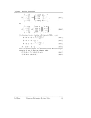
![7. Central Potential
Consider a particle having mass m in a central potential, namely a potential
V (r) that depends only on the distance
r= x2 + y 2 + z 2 (7.1)
from the origin. The Hamiltonian is given by
p2
H= + V (r) . (7.2)
2m
Exercise 7.0.1. Show that
[H, Lz ] = 0 , (7.3)
H, L2 = 0 . (7.4)
Solution 7.0.1. Using
[xi , pj ] = i δ ij , (7.5)
Lz = xpy − ypx , (7.6)
one has
p2 , Lz = p2 , Lz + p2 , Lz + p2 , Lz
x y z
= p2 , xpy − p2 , ypx
x y
= i (−2px py + 2py px )
=0,
(7.7)
and
r2 , Lz = x2 , Lz + y 2 , Lz + z 2 , Lz
= −y x2 , px + y 2 , py x
=0.
(7.8)
Thus Lz commutes with any smooth function of r2 , and consequently
[H, Lz ] = 0. In a similar way one can show that [H, Lx ] = [H, Ly ] = 0,
and therefore H, L2 = 0.](https://image.slidesharecdn.com/qmlecturenotes-130118222159-phpapp01/85/Quantum-Mechanics-Lecture-notes-195-320.jpg)
![Chapter 7. Central Potential
In classical physics the corresponding Poisson’s brackets relations hold
{H, Lx } = {H, Ly } = {H, Lz } = 0 , (7.9)
and
H, L2 = 0 . (7.10)
These relations imply that classically the angular momentum is a constant of
the motion [see Eq. (1.40)]. On the other in quantum mechanics, as we have
seen in section 2.12 of chapter 2, the commutation relations
[H, Lz ] = 0 , (7.11)
H, L2 = 0 , (7.12)
imply that it is possible to find a basis for the vector space made of common
eigenvectors of the operators H, L2 and Lz .
7.1 Simultaneous Diagonalization of the Operators H,
L2 and Lz
We start by proving some useful relations:
Exercise 7.1.1. Show that
L2 = r2 p2 − (r · p)2 + i r · p . (7.13)
Solution 7.1.1. The following holds
L2 = (xpy − ypx )2
z
= x2 p2 + y 2 p2 − xpy ypx − ypx xpy
y x
= x2 p2 + y 2 p2 − xpx ([py , y] + ypy ) − ypy ([px , x] + xpx )
y x
= x2 p2 + y 2 p2 − xpx ypy − ypy xpx + i (xpx + ypy ) .
y x
(7.14)
Using the relation
xpx xpx = x ([px , x] + xpx ) px = −i xpx + x2 p2 ,
x (7.15)
or
i xpx = x2 p2 − xpx xpx ,
x (7.16)
one has
Eyal Buks Quantum Mechanics - Lecture Notes 186](https://image.slidesharecdn.com/qmlecturenotes-130118222159-phpapp01/85/Quantum-Mechanics-Lecture-notes-196-320.jpg)
![7.2. The Radial Equation
Substituting into Eq. (7.34) yields an equation for ukl (r)
− 2 d2
+ Veff (r) ukl (r) = Ekl ukl (r) , (7.36)
2m dr2
where the effective potential Veff (r) is given by
2
l (l + 1)
Veff (r) = + V (r) . (7.37)
2mr2
The total wave function is thus given by
1
ϕklm (r) = ukl (r) Ylm (θ, φ) . (7.38)
r
Since the spherical harmonic Ylm (θ, φ) is assumed to be normalized [see Eq.
(6.114)], to ensure that ϕklm (r) is normalized we require that
∞ ∞
2
1= 2
drr |Rkl (r)| = dr |ukl (r)|2 . (7.39)
0 0
In addition solutions with different k are expected to be orthogonal, thus
∞
dru∗ ′ l (r) ukl (r) = δ kk′ .
k (7.40)
0
The wave functions ϕklm (r) represent common eigenstates of the operators
H, Lz and L2 , which are denoted as |klm and which satisfy the following
relations
ϕklm (r′ ) = r′ |klm , (7.41)
and
H |klm = Ekl |klm , (7.42)
L2 |klm = l (l + 1) 2 |klm , (7.43)
Lz |klm = m |klm . (7.44)
The following claim reveals an important property of the radial wavefunc-
tion near the origin (r = 0):
Claim. If the potential energy V (r) does not diverge more rapidly than 1/r
near the origin then
lim u (r) = 0 . (7.45)
r→0
Eyal Buks Quantum Mechanics - Lecture Notes 189](https://image.slidesharecdn.com/qmlecturenotes-130118222159-phpapp01/85/Quantum-Mechanics-Lecture-notes-199-320.jpg)

![7.3. Hydrogen Atom
We seek solutions of Eq. (7.67) that represent bound states, for which Ekl
is negative, and thus λkl is a nonvanishing real positive. In the limit ρ → ∞
the potential Vl (ρ) → 0, and thus it becomes negligibly small in comparison
with λkl [see Eq. (7.67)]. Therefore, in this limit the solution is expected to
be asymptotically proportional to e±λkl ρ . To ensure that the solution is nor-
malizable the exponentially diverging solution e+λkl ρ is excluded. Moreover,
as we have seen above, for small ρ the solution is expected to be proportional
to ρl+1 . Due to these considerations we express ukl (r) as
ukl (r) = y (ρ) ρl+1 e−λkl ρ . (7.69)
Substituting into Eq. (7.67) yields an equation for the function y (ρ)
d2 (l + 1) d 2 (1 − λkl (l + 1))
+2 − λkl + y=0. (7.70)
dρ2 ρ dρ ρ
Consider a power series expansion of the function y (ρ)
∞
y (ρ) = cq ρq . (7.71)
q=0
Substituting into Eq. (7.70) yields
∞ ∞
q (q − 1) cq ρq−2 + 2 (l + 1) qcq ρq−2
q=0 q=0
∞ ∞
−2λkl qcq ρq−1 + 2 (1 − λkl (l + 1)) cq ρq−1 = 0 ,
q=0 q=0
(7.72)
thus
cq 2 [λkl (q + l) − 1]
= . (7.73)
cq−1 q (q + 2l + 1)
We argue below that for physically acceptable solutions y (ρ) must be a poly-
nomial function [i.e. the series (7.71) needs to be finite]. To see this note that
for large q Eq. (7.73) implies that
cq 2λkl
lim = . (7.74)
q→∞ cq−1 q
Similar recursion relation holds for the coefficients of the power series expan-
sion of the function e2λkl ρ
∞
e2λkl ρ = cq ρq ,
˜ (7.75)
q=0
where
Eyal Buks Quantum Mechanics - Lecture Notes 193](https://image.slidesharecdn.com/qmlecturenotes-130118222159-phpapp01/85/Quantum-Mechanics-Lecture-notes-203-320.jpg)
![7.5. Solutions
9. Consider two (non-identical) particles having the same mass m moving
under the influence of a potential U (r), which is given by
1
U (r) = mω 2 r2 .
2
In addition, the particles interact with each other via a potential given
by
1 2 2
V (r1 , r2 ) = m (r1 − r2 ) ,
2
where r1 and r2 are the (three dimensional) coordinate vectors of the first
and second particle respectively. Find the eigenenergies of the system.
7.5 Solutions
1. In general the current density is given by Eq. (4.174). For a wavefunction
having the form
ψ (r) = α (r) eiβ(r) , (7.97)
where both α and β are real, one has
J= Im [α (∇α + iα∇β)]
µ
α2
= ∇β
µ
|ψ|2
= ∇β .
µ
(7.98)
a) The wavefunction ϕn,l,m (r) is given by
ψnlm (r, θ, φ) = Rnl (r) Ylm (θ, φ) = Rnl (r) Flm (θ) eimφ , (7.99)
where both Rnl and Flm are real, thus
2
ϕn,l,m (r)
Jn,l,m (r) = ∇ (mφ) . (7.100)
µ
In spherical coordinates one has
∂ ∂ ∂
∇=x ˆ +yˆ +ˆz
∂x ∂y ∂z
∂ ˆ1 ∂ + φ 1
ˆ ∂
=ˆ +θ
r ,
∂r r ∂θ r sin θ ∂φ
(7.101)
Eyal Buks Quantum Mechanics - Lecture Notes 197](https://image.slidesharecdn.com/qmlecturenotes-130118222159-phpapp01/85/Quantum-Mechanics-Lecture-notes-207-320.jpg)
![Chapter 7. Central Potential
√
5. The normalization constant is chosen to be A = 1/ 2. Since both states
|2, 1, −1 and |2, 1, 1 have the same energy the state |α is stationary.
The following holds
ψnlm (r, θ, φ) = Rnl (r) Ylm (θ, φ) , (7.114a)
3/2
1 r − r
R21 (r) = √ e 2a0 , (7.114b)
2a0 3a0
1 3
Y1−1 (θ, φ) = sin θe−iφ , (7.114c)
2 2π
1 3
Y11 (θ, φ) = − sin θeiφ , (7.114d)
2 2π
x = r sin θ cos φ . (7.114e)
In general
∞ 1 2π
′ ∗
′ ′ ′ 3
n l m | x |nlm = dr r Rn′ l′ Rnl d (cos θ) dφ sin θ cos φ Ylm
′ Ylm .
0 −1 0
(7.115)
thus
2π
2, 1, 1|x|2, 1, 1 ∝ dφ cos φ = 0 , (7.116)
0
2π
2, 1, −1|x|2, 1, −1 ∝ dφ cos φ = 0 , (7.117)
0
2π
2, 1, 1|x|2, 1, −1 ∝ dφ cos φe−2iφ = 0 , (7.118)
0
2π
2, 1, −1|x|2, 1, 1 ∝ dφ cos φe2iφ = 0 , (7.119)
0
and therefore
x (t) = 0 . (7.120)
6. The radial equation is given by [see Eq. (7.36)]
2
d2 l (l + 1) 2
− + + V (r) uk,l (r) = Ek,l uk,l (r) . (7.121)
2m dr2 2mr2
Since the centrifugal term l (l + 1) 2 /2mr2 is non-negative the ground
state is obtained with l = 0. Thus the ground state energy is [see Eq.
(4.160)]
Eyal Buks Quantum Mechanics - Lecture Notes 200](https://image.slidesharecdn.com/qmlecturenotes-130118222159-phpapp01/85/Quantum-Mechanics-Lecture-notes-210-320.jpg)
![Chapter 7. Central Potential
8. The state vector |γ is an eigenvector of the operators Lx , Ly , therefore it
is easy to see that it consequently must be an eigenvector of the operator
[Lx , Ly ] with a zero eigenvalue. Thus, since [Lx , Ly ] = i Lz , one has
Lz |γ = 0. Similarly, one finds that Lx |γ = Ly |γ = 0. Therefore, |γ
is also an eigenvector of the operator L2 = L2 + L2 + L2 with a zero
x y z
eigenvalue. Therefore the wavefunction has the form
R (r′ )
ψ (r′ ) = R (r′ ) Yl=0 θ′ , φ′ = √
m=0
, (7.133)
4π
where the radial function R (r′ ) is an arbitrary normalized function.
9. The Lagrangian is given by
m r2 + r2
˙1 ˙2 1 1
L= − mω2 r2 + r2 − m
1 2
2
(r1 − r2 )2 . (7.134)
2 2 2
In terms of center of mass r0 and relative r coordinates, which are given
by
r1 + r2
r0 = , (7.135)
2
r = r1 − r2 , (7.136)
the Lagrangian is given by
2 2
m r0 + 1 r
˙ 2˙ + r0 − 1 r
˙ 2˙
L=
2
2 2
1 1 1 1
− mω 2 r0 + r + r0 − r − m 2 2
r
2 2 2 2
m 2˙ 2 + 1 r2
r0 2 ˙ 1 1 1
= − mω 2 2r2 + r2 − m 2 r2
0
2 2 2 2
2 2
M r0 1
˙ µ˙
r 1
= − M ω2 r2 +
0 − µ ω 2 + 2 2 r2 ,
2 2 2 2
(7.137)
where the total mass M is given by
M = 2m , (7.138)
and the reduced mass [see also Eq. (7.50)] by
m
µ= . (7.139)
2
The Lagrangian L describes two decoupled three dimensional harmonic
oscillators. The first, which is associated with the center of mass motion,
has mass M = 2m and angular resonance frequency ω, whereas the
Eyal Buks Quantum Mechanics - Lecture Notes 202](https://image.slidesharecdn.com/qmlecturenotes-130118222159-phpapp01/85/Quantum-Mechanics-Lecture-notes-212-320.jpg)

![8. Density Operator
Consider an ensemble of N identical copies of a quantum system. The en-
semble can be divided into subsets, where all systems belonging to the same
subset have the same state vector. Let N wi be the number of systems having
state vector α(i) , where
0 ≤ wi ≤ 1 , (8.1)
and where
wi = 1 . (8.2)
i
The state vectors are all assumed to be normalized
α(i) α(i) = 1 . (8.3)
Consider a measurement of an observable A, having a set of eigenvalues
{an } and corresponding set of eigenvectors {|an }
A |an = an |an . (8.4)
The set of eigenvectors {|an } is assumed to be orthonormal and complete
am |an = δ nm , (8.5)
|an an | = 1 . (8.6)
n
Consider a measurement of the observable A done on a system that is ran-
domly chosen from the ensemble. The probability to choose a system having
state vector α(i) is wi . Given that the state vector is α(i) , the expectation
value of A is α(i) A α(i) [see Eq. (2.84)]. Thus, the expectation (average)
value of such a measurement done on a system that is randomly chosen from
the ensemble is given by
2
A = wi α(i) A α(i) = wi an α(i) an . (8.7)
i i n](https://image.slidesharecdn.com/qmlecturenotes-130118222159-phpapp01/85/Quantum-Mechanics-Lecture-notes-215-320.jpg)
![Tr (ρ) = bm | wi α(i) α(i) |bm
m i
= wi α(i) |bm bm | α(i)
i m
(i) (i)
= wi α α
i
= wi
i
=1.
(8.12)
Exercise 8.0.3. Show that for any normalized state |β the following holds
0 ≤ β| ρ |β ≤ 1 . (8.13)
Solution 8.0.3. Clearly, 0 ≤ β| ρ |β since
2
β| ρ |β = wi β α(i) α(i) |β = wi α(i) |β ≥0. (8.14)
i i
On the other hand, according to the Schwartz inequality [see Eq. (2.166)],
which is given by
| u |v | ≤ u |u v |v , (8.15)
one has
α(i) |β ≤ β |β α(i) α(i) = 1 . (8.16)
Moreover, i wi = 1, thus
2
β| ρ |β = wi α(i) |β ≤1. (8.17)
i
Exercise 8.0.4. Show that Tr ρ2 ≤ 1.
Solution 8.0.4. The fact that ρ is Hermitian (i.e., ρ† = ρ) guaranties the
existence of a complete orthonormal basis {|qm } of eigenvectors of ρ, which
satisfy
qm′ |qm = δ mm′ , (8.18)
|qm qm | = 1 , (8.19)
m
and
Eyal Buks Quantum Mechanics - Lecture Notes 207](https://image.slidesharecdn.com/qmlecturenotes-130118222159-phpapp01/85/Quantum-Mechanics-Lecture-notes-217-320.jpg)
![8.2. Quantum Statistical Mechanics
8.1 Time Evolution
Consider a density operator
ρ (t) = wi α(i) (t) α(i) (t) , (8.31)
i
where the state vectors α(i) (t) evolve in time according to
d α(i)
i = H α(i) , (8.32)
dt
d α(i)
−i = α(i) H , (8.33)
dt
where H is the Hamiltonian. Taking the time derivative yields
dρ 1
= wi H α(i) α(i) (t) − wi α(i) (t) α(i) H , (8.34)
dt i i i
thus
dρ 1
= − [ρ, H] . (8.35)
dt i
This result resembles the equation of motion (4.37) of an observable in the
Heisenberg representation, however, instead of a minus sign on the right hand
side, Eq. (4.37) has a plus sign.
Alternatively, the time evolution of the operator ρ can be expressed in
terms of the time evolution operator u (t, t0 ), which relates the state vector
at time α(i) (t0 ) with its value α(i) (t) at time t [see Eq. (4.4)]
α(i) (t) = u (t, t0 ) α(i) (t0 ) . (8.36)
With the help of this relation Eq. (8.31) becomes
ρ (t) = u (t, t0 ) ρ (t0 ) u† (t, t0 ) . (8.37)
8.2 Quantum Statistical Mechanics
Consider an ensemble of identical copies of a quantum system. Let H be the
Hamiltonian having a set of eigenenergies {Ei } and a corresponding set of
eigenstates {|i }, which forms an orthonormal and complete basis
H |i = Ei |i , (8.38)
|i i| = 1 . (8.39)
i
Eyal Buks Quantum Mechanics - Lecture Notes 209](https://image.slidesharecdn.com/qmlecturenotes-130118222159-phpapp01/85/Quantum-Mechanics-Lecture-notes-219-320.jpg)
![Chapter 8. Density Operator
Consider the case where the ensemble is assumed to be a canonical ensemble
in thermal equilibrium at temperature T . According to the laws of statistical
mechanics the probability wi to find an arbitrary system in the ensemble in
a state vector |i having energy Ei is given by
1 −βEi
wi = e , (8.40)
Z
where β = 1/kB T , kB is Boltzmann’s constant, and where
Z= e−βEi (8.41)
i
is the partition function.
Exercise 8.2.1. Show that the density operator ρ can be written as
e−βH
ρ= . (8.42)
Tr (e−βH )
Solution 8.2.1. According to the definition (8.9) one has
1
ρ= wi |i i| = e−βEi |i i| . (8.43)
i
Z i
Moreover, the following hold
Z= e−βEi = i| e−βH |i = Tr e−βH , (8.44)
i i
and
e−βEi |i i| = e−βH |i i| = e−βH |i i| = e−βH , (8.45)
i i i
thus
e−βH
ρ= . (8.46)
Tr (e−βH )
As will be demonstrated below [see Eq. (8.330)], the last result for ρ can
also be obtained from the principle of maximum entropy.
8.3 Problems
1. Consider a spin 1/2 in a magnetic field B = Bˆ and in thermal equilib-
z
rium at temperature T . Calculate S · u , where S is the vector operator
ˆ
of the angular momentum and where u is a unit vector, which can be
ˆ
described using the angles θ and φ
u = (sin θ cos φ, sin θ sin φ, cos θ) .
ˆ (8.47)
Eyal Buks Quantum Mechanics - Lecture Notes 210](https://image.slidesharecdn.com/qmlecturenotes-130118222159-phpapp01/85/Quantum-Mechanics-Lecture-notes-220-320.jpg)
![8.3. Problems
16. Consider a point particle having mass m in a potential of a harmonic
oscillator having angular frequency ω. Calculate the Wigner function
W (x′ , p′ ) for the case where the system is in the number state |n = 1 .
17. The Wigner function of a point particle moving in one dimension is
given by Eq. (8.63). Show that the marginal distributions x′ | ρ |x′ and
p′ | ρ |p′ of the position x and momentum p observables, respectively, are
given by
∞
x′ | ρ |x′ = −1
dp′ W (x′ , p′ ) , (8.64)
−∞
∞
p′ | ρ |p′ = −1
dx′ W (x′ , p′ ) . (8.65)
−∞
18. Homodyne Tomography - Consider a point particle having mass m
in a potential of a harmonic oscillator having angular frequency ω. The
normalized homodyne observable Xφ with a real phase φ is defined by
a† e−iφ + aeiφ
Xφ = √ , (8.66)
2
where a and a† are annihilation and creation operators [see Eqs. (5.9)
′
and (5.10)]. Let w Xφ be the normalized probability density of the
observable Xφ . The technique of homodyne detection can be used to
′
measure w Xφ for any given value of the phase φ. Show that the Wigner
′
function (8.63) can be extracted from the measured distributions w Xφ
for all values of φ.
19. Consider a harmonic oscillator in thermal equilibrium at temperature T ,
whose Hamiltonian is given by
p2 mω2 x2
H= + . (8.67)
2m 2
Calculate the matrix elements x′′ | ρ |x′ of the density operator in the
basis of eigenvectors of the position operator x.
20. A point particle having mass m is confined by the three dimensional
potential
1
V (r) = mω2 r2 , (8.68)
2
where r = x2 + y 2 + z 2 and where ω is a real constant. Calculate x
and x2 in thermal equilibrium at temperature T .
21. The entropy σ is defined by
σ = − Tr (ρ log ρ) . (8.69)
Show that σ is time independent.
Eyal Buks Quantum Mechanics - Lecture Notes 215](https://image.slidesharecdn.com/qmlecturenotes-130118222159-phpapp01/85/Quantum-Mechanics-Lecture-notes-225-320.jpg)
![8.3. Problems
b) Express ρ for the case of a microcanonical ensemble, for which the
only required constrain is (8.75).
c) Express ρ for the case of a canonical ensemble, for which in addition
to the constrain is (8.75) the expectation value of the Hamiltonian
H is required to have a given value, which is labeled by H .
d) Express ρ for the case of a grandcanonical ensemble, for which in ad-
dition to the constrain is (8.75) the expectation values of the Hamil-
tonian H and of the operator N are required to have given values,
which are labeled by H and N respectively. The operator N ,
which will be defined in chapter 16, is called the number of particles
operator.
25. Consider a point particle having mass m moving in one dimension under
the influence of the potential V (x). Calculate the canonical partition
function Zc [see Eq. (8.331)] in the classical limit, i.e. in the limit of high
temperature.
26. Let ρ be the density operator of a given system. The system is composed
of two subsystems, each having its own degrees of freedom, which are
labeled as ’1’ and ’2’ (e.g. a system of two particles). Let {|n1 1 } ({|n2 2 })
be an orthonormal basis spanning the Hilbert space of subsystem ’1’
(’2’). The set of vectors {|n1 , n2 }, where |n1 , n2 = |n1 1 |n2 2 , forms an
orthonormal basis spanning the Hilbert space of the combined system.
For a general operator O the partial trace over subsystem ’1’ is defined
by the following relation
Tr1 (O) ≡ 1 n1 | O |n1 1 . (8.77)
n1
Similarly, the partial trace over subsystem ’2’ is defined by
Tr2 (O) ≡ 2 n2 | O |n2 2 . (8.78)
n2
The observable A1 is a given Hermitian operator on the Hilbert space of
subsystem ’1’. Show that the expectation value of a measurement of A1
that is performed on subsystem ’1’ is given by
A1 = Tr1 (ρ1 A1 ) . (8.79)
where the operator ρ1 , which is given by
ρ1 = Tr2 ρ , (8.80)
is called the reduced density operator of subsystem ’1’.
27. Let ρ be the density operator of a given system. The total entropy of the
system σ is given by
σ = − Tr (ρ log ρ) . (8.81)
Eyal Buks Quantum Mechanics - Lecture Notes 217](https://image.slidesharecdn.com/qmlecturenotes-130118222159-phpapp01/85/Quantum-Mechanics-Lecture-notes-227-320.jpg)
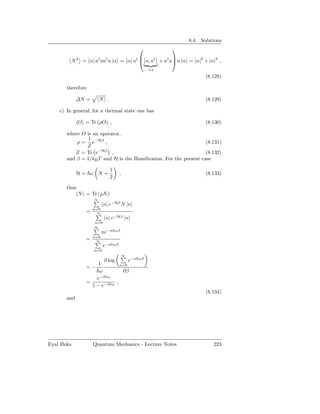

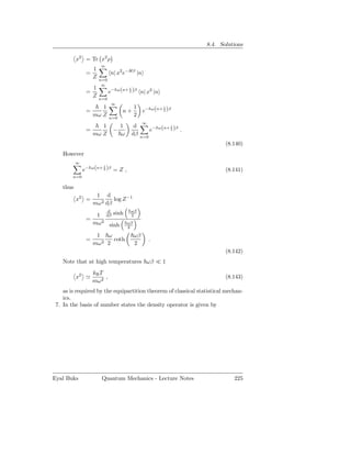
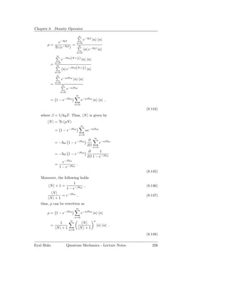
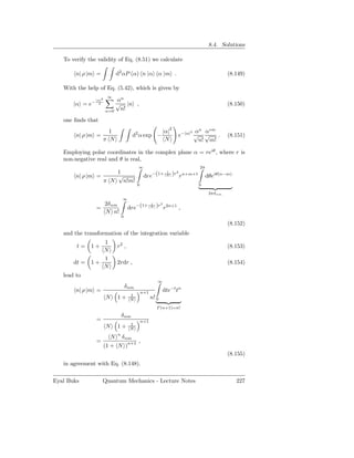
![Chapter 8. Density Operator
8. The density operator [see Eq. (8.51)] is given by
ρ= d2 α |α α| P (α) , (8.156)
where |α is a coherent state, d2 α denotes infinitesimal area in the α
complex plane,
2
1 |α|
P (α) = exp − , (8.157)
π N N
and where
e−β ω
N = (8.158)
1 − e−β ω
is the expectation value of the number operator N. Thus,
f (x′ ) = x′ | ρ |x′ = d2 αP (α) x′ |α α |x′ .
By employing the expression for the wave function ψα (x′ ) = x′ |α of a
coherent state which is given by [see Eq. (5.51)]
ψα (x′ ) = x′ |α
2
α∗2 − α2 mω 1/4 x′ − x α x′
= exp exp − +i p α ,
4 π 2∆xα
(8.159)
where
2
x α = α| x |α = Re (α) , (8.160)
mω
∆xα = α| (∆x)2 |α = , (8.161)
2mω
one finds that
Eyal Buks Quantum Mechanics - Lecture Notes 228](https://image.slidesharecdn.com/qmlecturenotes-130118222159-phpapp01/85/Quantum-Mechanics-Lecture-notes-238-320.jpg)

![8.4. Solutions
Pn α(i)
α(i) → . (8.174)
α(i) Pn α(i)
Thus, given that the system is initially in state α(i) the final density
operator is given by
(i) Pn α(i) α(i) Pn
ρ1 = α(i) Pn α(i)
n α(i) Pn α(i) α(i) Pn α(i)
= Pn α(i) α(i) Pn .
n
(8.175)
Averaging over all possible initial states thus yields
(i)
ρ1 = wi ρ1 = Pn wi α(i) α(i) Pn = Pn ρ0 Pn . (8.176)
i n i n
11. Since [V (t) , V (t′ )] = 0 the time evolution operator from initial time t0
to time t is given by
t
i
u (t, t0 ) = exp − dt′ V (t′ )
t0
ipi A
= exp x ,
(8.177)
where
t
pi = dt′ f (t′ ) . (8.178)
t0
While the initial state of the entire system at time t0 is given by |Ψ (t0 ) =
|ψi ⊗ |α , the final state at time t is given by
|Ψ (t) = u (t, t0 ) |Ψ (t0 )
= cn Jn |ψi ⊗ |an ,
n
(8.179)
where the operator Jn is given by
ipi an
Jn = exp x . (8.180)
Eyal Buks Quantum Mechanics - Lecture Notes 231](https://image.slidesharecdn.com/qmlecturenotes-130118222159-phpapp01/85/Quantum-Mechanics-Lecture-notes-241-320.jpg)
![Chapter 8. Density Operator
a) By introducing the identity operator dp′ |p′ p′ | = 1MD on the
Hilbert space of the MD, where |p′ are eigenvectors of the momen-
tum operator p, which is canonically conjugate to x, the state |Ψ (t)
can be expressed as
|Ψ (t) = cn dp′ p′ | Jn |ψ i |p′ ⊗ |an . (8.181)
n
With the help of the general identity (3.76), which is given by
dA
[p, A (x)] = −i , (8.182)
dx
where A (x) is a function of the operator x, one finds that
pJn |p′ = ([p, Jn ] + Jn p) |p′
= (pi an + p′ ) Jn |p′ ,
(8.183)
thus the vector Jn |p′ is an eigenvector of p with eigenvalue pi an +p′ .
Moreover, note that this vector, which is labeled as |p′ + pi an ≡
Jn |p′ , is normalized, provided that |p′ is normalized, since Jn is
unitary. The momentum wavefunction φ (p′ ) = p′ |ψi of the state
|ψi is related to the position wavefunction x′ |ψi by a Fourier trans-
form [see Eq. (3.60)]
∞ ip′ x′
dx′ e− x′ |ψ i
−∞
φ (p′ ) = √
2π
2
1 1 p′
= 1/2
exp − ,
π1/4 p0 2 p0
(8.184)
where
p0 = . (8.185)
x0
In terms of φ (p′ ) the state |Ψ (t) thus can be expressed as
|Ψ (t) = cn dp′ p′ − pi an |ψi |p′ ⊗ |an
n
= cn dp′ φ (p′ − pi an ) |p′ ⊗ |an .
n
(8.186)
Eyal Buks Quantum Mechanics - Lecture Notes 232](https://image.slidesharecdn.com/qmlecturenotes-130118222159-phpapp01/85/Quantum-Mechanics-Lecture-notes-242-320.jpg)
![Chapter 8. Density Operator
is called the reduced density operator. Note that ρR is an operator
on the Hilbert space of the MS. With the help of the expressions
|Ψ (∞) = cn′ dp′′ φ (p′′ − pi an′ ) |p′′ ⊗ |an′ , (8.192)
n
Ψ (∞)| = c∗ ′′
n dp′′′ φ∗ (p′′′ − pi an′′ ) an′′ | ⊗ p′′′ | , (8.193)
n′
one finds that
ρR = cn′ c∗ ′′
n dp′
n′ ,n′′
× φ (p′ − pi an′ ) φ∗ (p′ − pi an′′ ) |an′ an′′ | .
(8.194)
By employing the transformation of integration variable
2p′ − pi (an′ + an′′ )
x= , (8.195)
2p0
and its inverse
pi an′ + an′′
p′ = p0 x + , (8.196)
p0 2
one finds that
an′ −an′′ 2
−η2
dp′ φ (p′ − pi an′ ) φ∗ (p′ − pi an′′ ) = e 2
, (8.197)
thus
an′ −an′′ 2
−η2
ρR = cn′ c∗ ′′ e
n
2
|an′ an′′ | . (8.198)
n′ ,n′′
12. It is convenient to employ the coordinate transformation
x+y
x′ = √ , (8.199)
2
x−y
y′ = √ . (8.200)
2
The Lagrangian of the system can be written using these coordinates [see
Eq. (9.173)] as
L = L+ + L− , (8.201)
where
Eyal Buks Quantum Mechanics - Lecture Notes 234](https://image.slidesharecdn.com/qmlecturenotes-130118222159-phpapp01/85/Quantum-Mechanics-Lecture-notes-244-320.jpg)
![Chapter 8. Density Operator
Using the relations
x= a + a† , (8.214)
2mω
m ω
p=i −a + a† , (8.215)
2
a, a† = 1 , (8.216)
one finds that
2
x2 = a2 + a† + 2a† a + 1 , (8.217)
2mω
px 2
=i −a2 + a† − 1 . (8.218)
mω 2mω
a) Thus, for the ground state [see Eqs. (5.28) and (5.29)]
G (t) = [cos (ωt) − i sin (ωt)] = exp (−iωt) . (8.219)
2mω 2mω
b) The density operator ρ is given by Eq. (8.148)
∞ n
1 N
ρ= |n n| , (8.220)
N + 1 n=0 N +1
where
e−β ω
N = Tr (ρN ) = , (8.221)
1 − e−β ω
N = a† a, and where β = 1/kB T . Using the fact that ρ is diagonal
2
in the basis of number states one finds that a2 = a† = 0.
Combining all these results leads to
G (t) = [(2 N + 1) cos (ωt) − i sin (ωt)]
2mω
β ω
= coth cos (ωt) − i sin (ωt) .
2mω 2
(8.222)
14. The wave function of the coherent state |α is given by Eq. (5.51)
ψα (x′ ) = x′ |α
2
α∗2 − α2 mω 1/4 x′ − x α x′
= exp exp − +i p α .
4 π 2∆xα
(8.223)
where
Eyal Buks Quantum Mechanics - Lecture Notes 236](https://image.slidesharecdn.com/qmlecturenotes-130118222159-phpapp01/85/Quantum-Mechanics-Lecture-notes-246-320.jpg)
![8.4. Solutions
2
x α = α| x |α = α′ , (8.224)
mω
√
p α = α| p |α = 2 mωα′′ , (8.225)
α′ = Re (α) , (8.226)
α′′ = Im (α) , (8.227)
2
∆xα = α| (∆x) |α = , (8.228)
2mω
Using the definition (8.63) and the identity
∞
π 1 4ca+b2
exp −ax2 + bx + c dx = e4 a , (8.229)
a
−∞
one has
∞
1 p′ x′′ x′′ x′′
W (x′ , p′ ) = exp i x′ − |α α x′ + dx′′
2π −∞ 2 2
mω 1/2 ∞
= π
dx′′
2π −∞
′′ 2 ′′ 2
x′ − x − x α x′ + x − x α p′ − p α
− 2
2∆xα − 2
2∆xα +i x′′
×e
mω 1/2 ∞
= π
dx′′
2π −∞
′′ 2
−
(x′ − (
x α )2 + x
2 ) +i
p′ − p α
x′′
2(∆xα )2
×e ,
(8.230)
thus
2 2
x′ − x α p′ − p α
′1 −1
′
2 ∆xα −1
2 ∆pα
W (x , p ) = e , (8.231)
π
where [see Eq. (5.49)]
mω
∆pα = α| (∆p)2 |α = = . (8.232)
2 2∆xα
15. The density operator [see Eq. (8.51)] is given by
ρ= d2 α |α α| P (α) , (8.233)
where |α is a coherent state, d2 α denotes infinitesimal area in the α
complex plane,
Eyal Buks Quantum Mechanics - Lecture Notes 237](https://image.slidesharecdn.com/qmlecturenotes-130118222159-phpapp01/85/Quantum-Mechanics-Lecture-notes-247-320.jpg)
![Chapter 8. Density Operator
1 |α|2
P (α) = exp − , (8.234)
π N N
and where
e−β ω
N = (8.235)
1 − e−β ω
is the expectation value of the number operator N. Thus
W (x′ , p′ ) = d2 αP (α) Wα (x′ , p′ ) . (8.236)
where
∞
1 p′ x′′ x′′ x′′
Wα (x′ , p′ ) = exp i x′ − |α α x′ + dx′′ ,
2π −∞ 2 2
(8.237)
which is the Wigner function of a coherent state |α , was found to be
given by [see Eq. (8.231)]
2 2
x′ − x α p′ − p α
1 −1 −1
W (x′ , p′ ) =
2 ∆xα 2 ∆pα
e , (8.238)
π
where
2
x α = α| x |α = α′ = 2∆xα α′ , (8.239)
mω
√
p α = α| p |α = 2 mωα′′ = 2∆pα α′′ , (8.240)
α′ = Re (α) , (8.241)
α′′ = Im (α) , (8.242)
∆xα = α| (∆x)2 |α = , (8.243)
2mω
mω
∆pα = α| (∆p)2 |α = = . (8.244)
2 2∆xα
Thus W (x′ , p′ ) is given by
2 2
x′ − x α p′ − p α
′ ′ 1 2 − |α|
2
−1
2 ∆xα −1
2 ∆pα
W (x , p ) = 2 d αe N e
π N
x′ −2∆xα α′ 2 p′ −2∆xα α′ 2
1 − α −1
′2 ′′2
− αN − 1
= 2 dα′ e N 2 ∆xα
dα′′ e 2 ∆pα
.
π N
(8.245)
With the help of the identity (8.229) one thus finds that
Eyal Buks Quantum Mechanics - Lecture Notes 238](https://image.slidesharecdn.com/qmlecturenotes-130118222159-phpapp01/85/Quantum-Mechanics-Lecture-notes-248-320.jpg)
![Chapter 8. Density Operator
With the help of the identities (3.45) and (3.52) W (x′ , p′ ) can be ex-
pressed as
W (x′ , p′ )
′′ ′′
∞ ∞ ∞ (
p′ x′′ +p′′ x′ − x )−p′′′ (x′ + x2 )
1 2
= 2 dx′′ dp′′ dp′′′ ei p′′ | ρ |p′′′
(2π) −∞ −∞ −∞
p′′ p′′′
∞ ∞ x′ (p′′ −p′′′ ) ∞ x′′ p′ − −
1 ′′ ′′′ i ′′ ′′′ 1 ′′ i
2 2
= dp dp e p | ρ |p dx e .
2π −∞ −∞ 2π −∞
′′ ′′′
δ p′ − p2 − p2
(8.254)
The above result easily leads to (8.65)
∞
−1
dx′ W (x′ , p′ )
−∞
∞ ∞ ∞
p′′ p′′′ 1 x′ (p′′ −p′′′ )
= dp′′ dp′′′ p′′ | ρ |p′′′ δ p′ − − dx′ ei
−∞ −∞ 2 2 2π −∞
δ(p′′ −p′′′ )
′ ′
= p | ρ |p .
(8.255)
18. The normalized homodyne observable Xφ can be expressed in terms of
the dimensionless position and momentum operators X and P , which are
given by
a + a† a − a†
X= √ , P = √ , (8.256)
2 i 2
and which satisfy [X, P ] = i [see Eq. (5.13)], as
X − iP −iφ X + iP iφ
Xφ = e + e
2 2
= X cos φ − P sin φ .
(8.257)
The associated dimensionless momentum operator Pφ is defined as Pφ =
X sin φ + P cos φ, i.e.
Xφ cos φ − sin φ X
= , (8.258)
Pφ sin φ cos φ P
and the inverse transformation is given by
X cos φ sin φ Xφ
= . (8.259)
P − sin φ cos φ Pφ
Eyal Buks Quantum Mechanics - Lecture Notes 240](https://image.slidesharecdn.com/qmlecturenotes-130118222159-phpapp01/85/Quantum-Mechanics-Lecture-notes-250-320.jpg)
![8.4. Solutions
The marginal distributions Pr (X ′ ) for the dimensionless position X and
Pr (P ′ ) for the dimensionless momentum P are related to the Wigner
function (8.63) W (X ′ , P ′ ) by [see Eqs. (8.64) and (8.65)]
∞
Pr (X ′ ) = dP ′ W (X ′ , P ′ ) , (8.260)
−∞
∞
Pr (P ′ ) = dX ′ W (X ′ , P ′ ) , (8.261)
−∞
where Pr (A′ ) denotes the probability density of the random variable
A′ . Thus, the probability density Pr Xφ of Xφ , which is denoted as
′ ′
′
w Xφ , is given by
∞
′ ′
w Xφ = dPφ
−∞
′ ′
×W Xφ cos φ + Pφ sin φ, −Xφ sin φ + Pφ cos φ .
(8.262)
The last result (18) can be inverted using the so-called inverse Radon
˜
transform. The Fourier transformed Wigner function W (ξ, η) is ex-
pressed as
∞ ∞
˜ 1 ′
−iηP ′
W (ξ, η) = dX ′ dP ′ W (X ′ , P ′ ) e−iξX . (8.263)
2π −∞ −∞
′
The Fourier transform w (ζ) of the probability distribution w Xφ
˜ is
given by [see Eq. (18)]
∞
1 ′
w (ζ) = √
˜ dXφ w Xφ e−iζXφ
′ ′
2π −∞
∞ ∞
1 ′ ′
=√ dXφ dPφ
2π −∞ −∞
′
×W Xφ cos φ + Pφ sin φ, −Xφ sin φ + Pφ cos φ e−iζXφ .
′ ′
(8.264)
The variable transformation (8.259) leads to
∞ ∞
1
dX ′ dP ′ W (X ′ , P ′ ) e−iζ (X cos φ−P ′ sin φ)
′
w (ζ) = √
˜ ,
2π −∞ −∞
(8.265)
thus according to Eq. (8.263) the following holds
Eyal Buks Quantum Mechanics - Lecture Notes 241](https://image.slidesharecdn.com/qmlecturenotes-130118222159-phpapp01/85/Quantum-Mechanics-Lecture-notes-251-320.jpg)
![Chapter 8. Density Operator
√
w (ζ) =
˜ ˜
2π W (ζ cos φ, −ζ sin φ) . (8.266)
The last result (8.265) allows evaluating the Wigner function by inverse
Fourier transform
∞ ∞
1 ˜ ′ ′
W (X ′ , P ′ ) = dξdη W (ξ, η) eiξX +iηP . (8.267)
2π −∞ −∞
In polar coordinates this becomes
∞ π
1
dθ |ζ| W (ζ cos θ, ζ sin θ) eiζ (X cos θ+P ′ sin θ )
′
W (X ′ , P ′ ) = dζ ˜ ,
2π −∞ 0
(8.268)
thus with the help of Eq. (8.265) one finds that
∞ π
1
dθ |ζ| w (ζ) eiζ (X cos θ+P ′ sin θ )
′
W (X ′ , P ′ ) = 3/2
dζ ˜ ,
(2π) −∞ 0
(8.269)
thus [see Eq. (8.266)]
∞ π ∞
1 ′
cos θ+P ′ sin θ−x′ )
W (X ′ , P ′ ) = 2 dζ dθ dXφ |ζ| w Xφ eiζ (X
′ ′ φ .
(2π) −∞ 0 −∞
(8.270)
19. The density operator [see Eq. (8.51)] is given by
ρ= d2 α |α α| P (α) , (8.271)
where |α is a coherent state, d2 α denotes infinitesimal area in the α
complex plane,
1 |α|2
P (α) = exp − , (8.272)
π N N
and where
e−β ω
N = (8.273)
1 − e−β ω
is the expectation value of the number operator N . By employing the
expression for the wave function ψα (x′ ) = x′ |α of a coherent state
which is given by [see Eq. (5.51)]
Eyal Buks Quantum Mechanics - Lecture Notes 242](https://image.slidesharecdn.com/qmlecturenotes-130118222159-phpapp01/85/Quantum-Mechanics-Lecture-notes-252-320.jpg)
![8.4. Solutions
20. The dynamics along the x direction is governed by the Hamiltonian Hx
of a harmonic oscillator
p2
x 1
Hx = + mω 2 x2 . (8.292)
2m 2
By symmetry x = 0. The expectation value x2 was calculated in Eq.
(8.142) and found to be given by
1 ω ωβ
x2 = 2 2
coth . (8.293)
mω 2
21. In general, for any smooth function f (ρ) of ρ the following holds
f (ρ (t)) = u (t, t0 ) f (ρ (t0 )) u† (t, t0 ) . (8.294)
This can be shown by Taylor expanding the function f (ρ) as a power
series
∞
f (ρ (t)) = an (ρ (t))n , (8.295)
n=0
using Eq. (8.37) and the fact that u† (t, t0 ) u (t, t0 ) = 1, i.e. the unitarity
of the time evolution operator. By using this result for the function ρ log ρ
together with the general identity Tr (XY ) = Tr (Y X) [see Eq. (2.129)]
one easily finds that σ is time independent. This somewhat surprising
result can be attributed to the fact that the unitary time evolution that is
governed by the Schrödinger equation is symmetric under time reversal.
In the language of statistical mechanics it corresponds to a reversible
process, for which entropy is preserved.
22. Using the definition of the Pauli matrices (6.136) one finds that
1 1 + kz kx − iky
ρ= , (8.296)
2 kx + iky 1 − kz
and
1 1 + 2kz + k2 2 (kx − iky )
ρ2 = ,
4 2 (kx + iky ) 1 − 2kz + k2
where k2 = kx + ky + kz .
2 2 2
a) Note that for any k the following holds Tr (ρ) = 1. The requirement
that ρ is Hermitian, i.e. the requirement that ρ† = ρ, implies that
∗ ∗ ∗
kz = kz and kx − kx + i ky − ky = 0, thus kx , ky and kz are all real.
Moreover, the requirement that Tr ρ2 = 1 + k2 /2 ≤ 1 implies
that k2 ≤ 1.
b) For this case Tr ρ2 = 1, thus k2 = 1.
Eyal Buks Quantum Mechanics - Lecture Notes 245](https://image.slidesharecdn.com/qmlecturenotes-130118222159-phpapp01/85/Quantum-Mechanics-Lecture-notes-255-320.jpg)
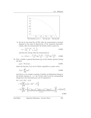
![Chapter 8. Density Operator
b) For the case of a microcanonical ensemble Eq. (8.327) yields ρ = 1/Z,
i.e. ρ is proportional to the identity operator.
c) For the case of a canonical ensemble Eq. (8.327) yields
1 −βH
ρc = e , (8.330)
Zc
where the canonical partition function Zc is given by
Zc = Tr e−βH , (8.331)
and where β labels the Lagrange multiplier associated with the given
expectation value H . By solving Eq. (8.76), which for this case is
given by [see also Eq. (8.329)]
1 ∂ log Zc
H = Tr He−βH = − . (8.332)
Zc ∂β
the Lagrange multiplier β can be determined. Note that the tem-
perature T is defined by the relation β = 1/kB T , where kB is the
Boltzmann’s constant.
d) For the case of a grandcanonical ensemble Eq. (8.327) yields
1 −βH+βµN
ρgc = e , (8.333)
Zgc
where the grandcanonical partition function Zgc is given by
Zgc = Tr e−βH+βµN . (8.334)
Here the Lagrange multiplier associated with the given expectation
value N is given by −βµ, where µ is known as the chemical poten-
tial. The average energy H is given by
H = Tr Hρgc
Tr He−β(H−µN)
=
Tr e−β(H−µN)
Tr − (H − µN ) e−β(H−µN) µ β Tr N e−βH+βµN
=− + ,
Tr e−β(H−µN) β Tr (e−βH+βµN )
thus
∂ log Zgc µ ∂ log Zgc
H =− + . (8.335)
∂β µ β ∂µ β
Similarly, the average number of particles N is given by
Tr N e−βH+βµN
N = Tr Nρgc = . (8.336)
Tr (e−βH+βµN )
Eyal Buks Quantum Mechanics - Lecture Notes 250](https://image.slidesharecdn.com/qmlecturenotes-130118222159-phpapp01/85/Quantum-Mechanics-Lecture-notes-260-320.jpg)
![Chapter 8. Density Operator
Note that the this result can be also obtained by taking the limit → 0,
for which the operator x and p can be considered as commuting operators
(recall that [x, p] = i ), and consequently in this limit e−βH can be
factored in the same way [see Eq. (8.342)].
26. The measurement of the observable A1 is describe by the its extension,
which is given by A1 12 , where 12 is the identity operator on subsystem
’2’. Thus with the help of Eq. (8.8) one finds that
A1 = Tr (ρA1 12 )
= n1 , n2 | ρA1 12 |n1 , n2
n1 ,n2
= 1 n1 | 2 n2 | ρ |n2 2 A1 |n1 1
n1 n2
= Tr1 (ρ1 A1 ) .
(8.345)
27. In terms of the matrix elements ρn1 ,n2 ,m1 ,m2 of the operator ρ, which are
given by
ρ(n1 ,n2 ),(m1 ,m2 ) = n1 , n2 | ρ |m1 , m2 , (8.346)
the matrix elements of ρ1 and ρ2 are given by
(ρ1 )n1 ,m1 = ρ(n1 ,n2 ),(m1 ,n2 ) , (8.347)
n2
and
(ρ2 )n2 ,m2 = ρ(n1 ,n2 ),(n1 ,m2 ) . (8.348)
n1
In general ρ is Hermitian, i.e.
∗
ρ(n1 ,n2 ),(m1 ,n2 ) = ρ(m1 ,n2 ),(n1 ,n2 ) , (8.349)
and therefore
∗ ∗
(ρ1 )n1 ,m1 = ρ(n1 ,n2 ),(m1 ,n2 )
n2
= ρ(m1 ,n2 ),(n1 ,n2 )
n2
= (ρ1 )m1 ,n1 ,
(8.350)
i.e. ρ1 is also Hermitian, and similarly ρ2 is also Hermitian. Thus the
eigenvalues of ρ1 and ρ2 are all real. Moreover, these eigenvalues represent
Eyal Buks Quantum Mechanics - Lecture Notes 252](https://image.slidesharecdn.com/qmlecturenotes-130118222159-phpapp01/85/Quantum-Mechanics-Lecture-notes-262-320.jpg)
![Chapter 8. Density Operator
thus
− wn1 ,n2 log wn1 ,n2
n1 ,n2
wk
= | n1 , n2 |k |2 wk log
n1 ,n2
wn1 ,n2
k
+σ .
(8.375)
Furthermore, according to inequality (8.369) the following holds
2 wk
| n1 , n2 |k | wk log
wn1 ,n2
k
wk wk
= | n1 , n2 |k |2 wn1 ,n2 log
wn1 ,n2 wn1 ,n2
k
wk
≥ | n1 , n2 |k |2 wn1 ,n2 −1 ,
wn1 ,n2
k
| n1 , n2 |k |2 wk − wn1 ,n2 | n1 , n2 |k |2
k k
=0.
(8.376)
These results together with inequality (8.373) yield
σ1 + σ2 ≥ σ . (8.377)
28. With the help of Eq. (8.92), which is given by
e−Hβ
ρ= = p+ |+ +| + p− |− −| , (8.378)
Tr (e−Hβ )
where the probabilities p+ and p− are given by
ωβ
e∓ 2
p± = ωβ ωβ , (8.379)
e− 2 +e 2
ω = |e| B/me c is the Larmor frequency [see Eq. (4.22)] and where β =
1/kB T , one finds that
σ = −p+ log p+ − p− log p−
ωβ ωβ ωβ
1 − tanh 2 1 − tanh 2 1 + tanh 2 1 + tanh ωβ2
=− log − log .
2 2 2 2
(8.380)
Eyal Buks Quantum Mechanics - Lecture Notes 256](https://image.slidesharecdn.com/qmlecturenotes-130118222159-phpapp01/85/Quantum-Mechanics-Lecture-notes-266-320.jpg)
![9.1. The Level En
one finds that
Pk E − En Pn − k′ =n Ek′ Pk′
R (E − H0 ) =
E − Ek
k=n
Pk (E − Ek )
=
k=n
E − Ek
= Qn ,
(9.16)
and similarly
(E − H0 ) R = Qn . (9.17)
The last two results suggest that the operator R can be considered as the
inverse of E − H0 in the subspace of eigenvalue zero of the projector Pn
(which is the subspace of eigenvalue unity of the projector Qn ). Multiplying
Eq. (9.9) from the left by R yields
˜
λRV |α = R (E − H0 ) |α . (9.18)
With the help of Eq. (9.16) one finds that
˜
λRV |α = Qn |α . (9.19)
Since Pn = 1 − Qn [see Eq. (9.8)] the last result implies that
˜ ˜
Pn |α = |α − λRV |α = 1 − λRV |α , (9.20)
which leads to Eq. (9.11)
−1
˜
|α = 1 − λRV Pn |α . (9.21)
Note that Eq. (9.11) can be expanded as power series in λ
˜ ˜ ˜
|α = 1 + λRV + λ2 RV RV + · · · Pn |α . (9.22)
9.1.1 Nondegenerate Case
In this case gn = 1 and
Pn = |n n| . (9.23)
In general the eigenvector |α is determined up to multiplication by a con-
stant. For simplicity we choose that constant to be such that
Eyal Buks Quantum Mechanics - Lecture Notes 259](https://image.slidesharecdn.com/qmlecturenotes-130118222159-phpapp01/85/Quantum-Mechanics-Lecture-notes-269-320.jpg)

![Chapter 9. Time Independent Perturbation Theory
p2 mω2 x2
H0 = + . (9.40)
2m 2
and where
mω
V =λ ω x. (9.41)
The eigenvectors and eigenvalues of the Hamiltonian H0 , which describes a
one dimensional harmonic oscillator, are given by
H0 |n = En |n , (9.42)
where n = 0, 1, , 2 · · · , and where
1
En (λ = 0) = ω n + . (9.43)
2
Note that, as was shown in chapter 5 [see Eq. (5.145)], the eigenvectors
and eigenvalues of H can be found analytically for this particular case. For
the sake of comparison we first derive this exact solution. Writing H as
p2 mω 2 x2 mω
H= + +λ ω x
2m 2
2
p2 mω 2 1
= + x+λ − ωλ2 ,
2m 2 mω 2
(9.44)
one sees that H describes a one dimensional harmonic oscillator (as H0 also
does). The exact eigenenergies are given by
1
En (λ) = En (λ = 0) − ωλ2 , (9.45)
2
and the corresponding exact wavefunctions are
x′ |n (λ) = x′ + λ |n . (9.46)
mω
Using identity (3.19), which is given by
J (∆x) |x′ = |x′ + ∆x , (9.47)
where J (∆x) is the translation operator, the exact solution (9.46) can be
rewritten as
x′ |n (λ) = x′ | J −λ |n , (9.48)
mω
Eyal Buks Quantum Mechanics - Lecture Notes 262](https://image.slidesharecdn.com/qmlecturenotes-130118222159-phpapp01/85/Quantum-Mechanics-Lecture-notes-272-320.jpg)

![9.4. Solutions
18. Consider the Hamiltonian H, which is given by
˜
H = H0 + λV , (9.89)
where λ ∈ R. The set {|k } of eigenvectors of H0 with corresponding
eigenvalues {Ek }, which satisfy
H0 |k = Ek |k , (9.90)
is assumed to form an orthonormal basis for the vector space, i.e.
k′ |k = δ kk′ . (9.91)
Consider the transformation
HR = eL He−L , (9.92)
where the operator L is assumed to be anti Hermitian, i.e. L† = −L, in
order to ensure that eL is unitary. Show that to second order in λ the
matrix elements k| HR |k′′ are given by
λ2 ˜ ˜ 1 1
k| HR |k′′ = Ek δ k,k′ + k| V |k′′ k′′ | V |k′ − ,
2 Ek − Ek ′′ Ek ′′ − Ek′
k′′
(9.93)
provided that the following condition is satisfied
˜
λV + [L, H0 ] = 0 . (9.94)
Note that to first order in λ the following holds k| HR |k′′ = k| H0 |k′′ ,
˜
thus, in spite of the fact that the perturbation λV is first order in λ, the
transformed Hamiltonian HR depends on λ only to second order.
9.4 Solutions
1. The radial force acting on the electron is found using Gauss’ theorem
e2
r2 r > ρ0
Fr (r) = e2 r 3 . (9.95)
r2 ρ r ≤ ρ0
0
The potential energy V (r) is found by integrating Fr (r) and by requiring
that V (r) is continuous at r = ρ0
2
− er r > ρ0
V (r) = e2 r
2 . (9.96)
2ρ ρ − 3 r ≤ ρ0
0 0
Eyal Buks Quantum Mechanics - Lecture Notes 269](https://image.slidesharecdn.com/qmlecturenotes-130118222159-phpapp01/85/Quantum-Mechanics-Lecture-notes-279-320.jpg)


![Chapter 9. Time Independent Perturbation Theory
nx − ny nx + ny + 1 2
En+ ,n− = ω nx + ny + 1 + β− β + O β3 .
2 8
(9.177)
8. Using Eqs. (5.28) and (5.29) one finds that
m| V |n = β n (n − 1)δ m,n−2 + β (n + 1) (n + 2)δ m,n+2 , (9.178)
thus
1 | m| V |n |2
En (β) = ω n + + n| V |n + + O β3
2 En (0) − Em (0)
m=n
=0
2
1 β
= ω n+ + [n (n − 1) − (n + 1) (n + 2)] + O β 3
2 2 ω
2
1 β
= ω n+ 1−2 + O β3 .
2 ω
(9.179)
9. In general the subspace of angular momentum states with J = 1 is
spanned by the basis
{|j = 1, m = −1 , |j = 1, m = 0 , |j = 1, m = 1 } , (9.180)
and the following holds
j ′ , m′ | Jz |j, m = m δ j′ ,j δ m′ ,m , (9.181)
j ′ , m′ | J2 |j, m = j (j + 1) 2 δ j ′ ,j δ m′ ,m , (9.182)
j ′ , m′ | J± |j, m = (j ∓ m) (j ± m + 1)δ j ′ ,j δ m′ ,m±1 , (9.183)
J± = Jx ± iJy . (9.184)
In matrix form
10 0
Jz = 0 0 0 ,
˙ (9.185)
0 0 −1
100
J2 = 2 2 0 1 0 ,
˙ (9.186)
001
√ 010
J+ =˙ 20 0 1 , (9.187)
000
√ 000
J− =˙ 21 0 0 . (9.188)
010
Eyal Buks Quantum Mechanics - Lecture Notes 280](https://image.slidesharecdn.com/qmlecturenotes-130118222159-phpapp01/85/Quantum-Mechanics-Lecture-notes-290-320.jpg)

![9.4. Solutions
√
n, +| V |n, + n, +| V |n + 1, − √0 g n+1
= ,
n + 1, −| V |n, + n + 1, −| V |n + 1, − g n+1 0
(9.208)
thus to first order in g the eigenenergies are given by
√
E = ω (n + 1) ± g n + 1 . (9.209)
11. Using creation and annihilation operators one has
p2 + p2
x y 1
H0 = + mω 2 x2 + y 2 = ω (Nx + Ny + 1) , (9.210)
2m 2
where Nx = a† ax , Ny = a† ay , and
x y
βω
V = L2
z
βω
= (xpy − ypx )2
βω 2
= i ax a† − a† ay
y x
2 2
= −β ω a2 a†
x y + a†
x a2 − ax a† a† ay − a† ax ay a†
y x y x y
2 2
= −β ω a2 a†
x y + a†
x a2 − (1 + Nx ) Ny − Nx (1 + Ny ) .
y
(9.211)
a) For the case β = 0 the ground state |0, 0 is nondegenerate and has
energy E0,0 = ω. Since V |0, 0 = 0 one finds to second order in β
1 | nx , ny | V |0, 0 |2
E0,0 = ω+ 0, 0| V |0, 0 − = ω+O β 3 .
ω nx + ny
nx ,ny =0,0
(9.212)
b) For the case β = 0 the first excited state is doubly degenerate
H0 |1, 0 = 2 ω |1, 0 , (9.213)
H0 |0, 1 = 2 ω |0, 1 . (9.214)
The matrix of V in the basis {|1, 0 , |0, 1 } is given by
1, 0| V |1, 0 1, 0| V |0, 1
0, 1| V |1, 0 0, 1| V |0, 1
1, 0| [(1 + Nx ) Ny + Nx (1 + Ny )] |1, 0 0
=β ω
0 0, 1| [(1 + Nx ) Ny + Nx (1 + Ny )] |0, 1
10
=β ω .
01
(9.215)
Eyal Buks Quantum Mechanics - Lecture Notes 283](https://image.slidesharecdn.com/qmlecturenotes-130118222159-phpapp01/85/Quantum-Mechanics-Lecture-notes-293-320.jpg)

![Chapter 9. Time Independent Perturbation Theory
m0 | V |n0
|n1 = |m0 . (9.275)
m
λn0 − λm0
Multiplying Eq. (9.264) by n0 | yields
λn2 = n0 | V |n1 − λn1 n0 |n1 , (9.276)
or using Eq. (9.275)
n0 | V |m0 m0 | V |n0
λn2 = . (9.277)
m
λn0 − λm0
Thus, using this result together with Eq. (9.273) one finds
λ = λn0 + n0 | V |n0
2 n0 | V |m0 m0 | V |n0 3
+ +O .
m
λn0 − λm0
(9.278)
18. The condition [9.94] together with Eq. (9.90) can be used to evaluate the
matrix elements of L
˜
k| V |k′
k| L |k′ = λ . (9.279)
Ek − Ek′
With the help of Eq. (2.173) one finds that
˜ ˜ 1 ˜
HR = H0 +λV +[L, H0 ]+ L, λV + L, L, H0 + λV +· · · . (9.280)
2!
Thus, for the case where condition (9.94) is satisfied the following holds
[note that according to Eq. (9.279) L = O (λ)]
˜ 1
HR = H0 + L, λV + [L, [L, H0 ]] + O λ3
2!
1 ˜ + O λ3 .
= H0 + L, λV
2
(9.281)
where Eq. (9.94) has been employed in the last step. The last result
together with Eq. (9.279) and the closure relation 1 = k′′ |k′′ k′′ | [see
Eq. (2.23)] lead to
1 ˜
k| HR |k′′ = k| H0 |k′ + k| L, λV |k′ + O λ3
2
λ2 ˜ ′′ k′′ | V |k′
′′ k| V |k
˜ 1
− 1
k Ek −Ek′′ Ek′′ −Ek′
= Ek δ k,k′ + + O λ3 .
2
(9.282)
Eyal Buks Quantum Mechanics - Lecture Notes 290](https://image.slidesharecdn.com/qmlecturenotes-130118222159-phpapp01/85/Quantum-Mechanics-Lecture-notes-300-320.jpg)
![10. Time-Dependent Perturbation Theory
Recall that the time evolution of a state vector |α is governed by the
Schrödinger equation (4.1)
d |α
i = H |α , (10.1)
dt
where the Hermitian operator H = H† is the Hamiltonian of the system. The
time evolution operator u (t, t0 ) [see Eq. (4.4)] relates the state vector |α (t0 )
at time t0 with its value |α (t) at time t
|α (t) = u (t, t0 ) |α (t0 ) . (10.2)
As we have seen in chapter 4, when the Hamiltonian is time independent
u (t, t0 ) is given by
i (t − t0 )
u (t, t0 ) = exp − H . (10.3)
In this chapter we consider the more general case where H is allowed to vary
in time. We first derive a formal expression for the time evolution operator
u (t, t0 ) applicable for general H. Then we present the perturbation theory
expansion of the time evolution operator, and discuss approximation schemes
to evaluated u (t, t0 ).
10.1 Time Evolution
Dividing the time interval (t0 , t) into N sections of equal duration allows
expressing the time evolution operator as
N
u (t, t0 ) = u (tn , tn−1 ) , (10.4)
n=1
where
tn = t0 + nǫ , (10.5)](https://image.slidesharecdn.com/qmlecturenotes-130118222159-phpapp01/85/Quantum-Mechanics-Lecture-notes-301-320.jpg)

![Chapter 10. Time-Dependent Perturbation Theory
Solution 10.3.1. Since H1 (t) is Hermitian one finds that
| O (t) |2
iλ t λ2 t t′
= 1− dt′ H1I (t′ ) − 2
dt′ dt′′ H1I (t′ ) H1I (t′′ )
t0 t0 t0
iλ t λ2 t t′
× 1+ dt′ H1I (t′ ) − 2
dt′ dt′′ H1I (t′′ ) H1I (t′ )
t0 t0 t0
2
λ2 t
′ ′
= 1+ 2
dt H1I (t )
t0
λ2 t t′
− 2
dt′ dt′′ ( H1I (t′ ) H1I (t′′ ) + H1I (t′′ ) H1I (t′ ) )
t0 t0
+O λ3 ,
(10.18)
or
2
2 λ2 t
′ ′
| O (t) | = 1 + 2
dt H1I (t )
t0
λ2 t t
− 2
dt′ dt′′ H1I (t′ ) H1I (t′′ ) ,
t0 t0
(10.19)
thus
λ2 t t
| O (t) |2 = 1 − 2
dt′ dt′′
t0 t0
× [ H1I (t ) H1I (t′′ ) − H1I (t′ ) H1I (t′′ ) ] ,
′
(10.20)
or
λ2 t t
| O (t) |2 = 1 − 2
dt′ dt′′ ∆H1I (t′ ) ∆H1I (t′′ ) , (10.21)
t0 t0
where
∆H1I (t) = H1I (t) − H1I (t) . (10.22)
10.4 Transition Probability
Consider the case where the unperturbed Hamiltonian H0 is time indepen-
dent. The eigenvectors of H0 are denoted as |an , and the corresponding
eigenenergies are denoted as En
Eyal Buks Quantum Mechanics - Lecture Notes 294](https://image.slidesharecdn.com/qmlecturenotes-130118222159-phpapp01/85/Quantum-Mechanics-Lecture-notes-304-320.jpg)
![10.4. Transition Probability
where ∆E = ω mn .
0.8
0.6
0.4
0.2
-10 -8 -6 -4 -2 0 2 4 x 6 8 10
2
The function f (x) = sin x/x2 .
10.4.2 The Near-Resonance Case
In this case H1 is assumed to be given by
′ ′
H1 (t′ ) = Ke−iωt + K† eiωt , (10.36)
where K is an operator that is assumed to be time independent (after being
turned on at t0 = 0), and where the angular frequency ω is a positive constant.
The transition probability is given by [see Eq. (10.28)]
(ω mn −ω)t (ωmn −ω)t
i
4 e 2 sin 2 am | λK |an
pnm = 2 ω mn − ω
(ω mn +ω)t 2
(ωmn +ω)t
ei 2 sin 2 am | λK† |an
+ ,
ω mn + ω
(10.37)
We refer to the case where ω = ω mn as absorption resonance, and to the
case where ω = −ωmn as stimulated emission resonance. Near any of these
resonances ω ≃ ±ω mn the dominant contribution to pnm comes from only
one out of the two terms in Eq. (10.37), thus
2 (ω −ω)t
42 sin mn 2 | am | λK |an |2 ω mn ≃ ω
2
(ωmn −ω)
pnm ≃ (ω +ω)t . (10.38)
4 sin2 mn 22
a | λK† |a
2
ω ≃ −ω
2
(ωmn +ω) m n mn
In the long time limit, i.e. in the limit t → ∞, the probability pnm is
found using Eq. (10.33) to be proportional to the time t, i.e. pnm = wnm t,
where the transition rate wnm is given by
Eyal Buks Quantum Mechanics - Lecture Notes 297](https://image.slidesharecdn.com/qmlecturenotes-130118222159-phpapp01/85/Quantum-Mechanics-Lecture-notes-307-320.jpg)
![Chapter 10. Time-Dependent Perturbation Theory
2π
2 δ (ωmn − ω) | am | λK |an |2 ω mn ≃ ω
wnm ≃ 2π 2 . (10.39)
2 δ (ω mn + ω) am | λK† |an ω mn ≃ −ω
In many cases of interest the final state |am lie in a band of dense states. Let
wn be the total transition rate from the initial state |an . Assume that the
matrix element am | λK |an does not vary significantly as a function of the
energy Em . For this case the total rate wn can be expressed in terms of the
density of states g (Em ) (i.e. number of states per unit energy) in the vicinity
of the final state |am [see Eq. (10.39)] as
2π
wn = g (Em ) | am | λK |an |2 , (10.40)
where Em = En + ω. This result is known as the Fermi’s golden rule.
10.4.3 H1 is Separable
For this case it is assumed that H1 can be expressed as
¯
H1 (t′ ) = f (t′ ) H1 , (10.41)
¯
where f (t′ ) is a real function of time and where H1 is time independent
Hermitian operator. To lowest nonvanishing order in λ Eq. (10.28) yields
t 2
1 ′
¯ 2
pnm = 2
dt′ eiωmn t f (t′ ) am | λH1 |an . (10.42)
0
10.5 Problems
1. Find the exact time evolution operator u (t, 0) of the Hamiltonian H,
which is given by
H = H0 + Hp , (10.43)
where
H0 = ωa† a , (10.44)
Hp = i ωζ (t) e2i(ωt−φ) a2 − e−2i(ωt−φ) a†2 , (10.45)
a and a† are the annihilation and creation operators (as defined in chapter
5), ω is positive, φ is real and ζ (t) is an arbitrary real function of time t.
Eyal Buks Quantum Mechanics - Lecture Notes 298](https://image.slidesharecdn.com/qmlecturenotes-130118222159-phpapp01/85/Quantum-Mechanics-Lecture-notes-308-320.jpg)
![Chapter 10. Time-Dependent Perturbation Theory
2
xe−( τ ) ,
t
λH1 (t) = λ (10.52)
τa
where λ ≪ 1 and where τ is a positive constant having the dimensions
of time, is applied. Calculate the probability to find the particle in the
first excited state in the limit t → ∞.
10.6 Solutions
1. Expressing the ket vector state as
|ψ = e−iH0 t/ |ψI , (10.53)
and substituting into the Schrödinger equation, which is given by
d |ψ
i = (H0 + Hp ) |ψ , (10.54)
dt
yield
d |ψI
i = HI |ψI . (10.55)
dt
where HI , which is given by
HI = eiH0 t/ Hp e−iH0 t/ , (10.56)
is the interaction picture representation of Hp . With the help of the vector
identity (2.173), which is given by
1 1
eL Ae−L = A + [L, A] + [L, [L, A]] + [L, [L, [L, A]]] + · · · , (10.57)
2! 3!
and the relations
it
H0 , a2 = −2iωta2 , (10.58)
and
it
H0 , a†2 = 2iωta†2 , (10.59)
one finds that
eiH0 t/ a2 e−iH0 t/ = a2 e−2iωt , (10.60)
iH0 t/ †2 −iH0 t/ †2 2iωt
e a e =a e , (10.61)
thus
Eyal Buks Quantum Mechanics - Lecture Notes 300](https://image.slidesharecdn.com/qmlecturenotes-130118222159-phpapp01/85/Quantum-Mechanics-Lecture-notes-310-320.jpg)
![10.6. Solutions
HI = i ζ (t) e−2iφ a2 − e2iφ a†2 . (10.62)
Since [HI (t) , HI (t′ )] = 0 the solution of Eq. (10.55) is given by
t
i
|ψI (t) = exp − dt′ HI (t′ ) |ψI (0)
0
= S (ξ, φ) |ψI (0) ,
(10.63)
where
S (ξ, φ) = exp ξ e−2iφ a2 − e2iφ a†2 , (10.64)
and where
t
ξ= dt′ ζ (t′ ) , (10.65)
0
and thus the time evolution operator is thus given by
u (t, 0) = e−iH0 t/ S (ξ, φ) . (10.66)
2. To lowest nonvanishing order in the perturbation expansion one finds
using Eq. (10.38) together with Eqs. (5.11), (5.28) and (5.29) that
(ω −ω)t
2α2 sin2 0 2
pn0 (t) = δ n,1 . (10.67)
m ω (ω 0 − ω)2
3. To lowest nonvanishing order in perturbation expansion Eq. (10.42) yields
pn0 = µδ n,1 , (10.68)
where
∞ 2
1 ′
µ= dt′ eiω0 t f (t′ )
2m ω 0 −∞
α2 1 2 2
= e− 2 τ ω0 .
2m ω 0
(10.69)
The exact result is found from Eq. (5.315)
e−µ µn
pn = . (10.70)
n!
To first order in µ both results agree.
Eyal Buks Quantum Mechanics - Lecture Notes 301](https://image.slidesharecdn.com/qmlecturenotes-130118222159-phpapp01/85/Quantum-Mechanics-Lecture-notes-311-320.jpg)
![Chapter 10. Time-Dependent Perturbation Theory
4. While the exact result is [see Eq. (6.284)]
ωt
p++ (t) = cos2 , (10.71)
2
Eq. (10.21) yields
1 t t
p++ (t) = 1 − 2
dt′ dt′′ +; ˆ| (ωSx − +; ˆ| ωSx |+; ˆ )2 |+; ˆ
z z z z
0 0
ω 2 +; ˆ| Sx |+; ˆ
z 2 z t t
= 1− 2
dt′ dt′′
0 0
2
ωt
= 1− .
2
(10.72)
′
5. The normalized wavefunctions ψn (x ) of the well’s energy eigenstates are
given by
2 nπx′
ψn (x′ ) = sin , (10.73)
a a
and the corresponding eigenenergies are
2 2 2
π n
En = , (10.74)
2ma2
where n = 1, 2, · · · . The transition probability is calculated to lowest
ˆ
nonvanishing order in λ with the help of Eq. (10.42)
2 t 2 2
λ ′ i(E2 −E1 )t′ / − t′
p2,1 = dt e e τ
τa 0
2
2 a 2πx′ πx′
× dx′ x′ sin sin ,
a 0 a a
(10.75)
thus [see Eq. (8.229)
256λ2 9π4 2 τ 2
p2,1 = exp − . (10.76)
81π3 8m2 a4
Eyal Buks Quantum Mechanics - Lecture Notes 302](https://image.slidesharecdn.com/qmlecturenotes-130118222159-phpapp01/85/Quantum-Mechanics-Lecture-notes-312-320.jpg)
![11. WKB Approximation
The theory of geometrical optics provides an approximated solution to
Maxwell’s equation that is valid for systems whose typical size scales are
much larger than the wavelength λ of electromagnetic waves. In 1926 using a
similar approach the physicists Wentzel, Kramers and Brillouin (WKB) in-
dependently found an approximated solution to the Schrödinger equation in
the coordinate representation for the case where the wavelength associated
with the wavefunction (to be defined below) can be considered as short. Be-
low the WKB approximation is discussed for the time independent and one
dimensional case. This chapter is mainly based on Ref. [3].
11.1 WKB Wavefunction
Consider a point particle having mass m moving under the influence of a one-
dimensional potential V (x). The time independent Schrödinger equation for
the wavefunction ψ (x) is given by [see Eq. (4.50)]
d2 ψ (x) 2m
+ 2 (E − V (x)) ψ (x) = 0 , (11.1)
dx2
where E is the energy. In terms of the local momentum p (x), which is defined
by
p (x) = 2m (E − V (x)) , (11.2)
the Schrödinger equation becomes
d2 ψ (x) p 2
+ ψ (x) = 0 . (11.3)
dx2
Using the notations
ψ (x) = eiW (x)/ , (11.4)
and the relation
2
d2 ψ (x) i d2 W 1 dW
= − ψ (x) , (11.5)
dx2 dx2 dx](https://image.slidesharecdn.com/qmlecturenotes-130118222159-phpapp01/85/Quantum-Mechanics-Lecture-notes-313-320.jpg)
![Chapter 11. WKB Approximation
1
J= |C+ |2 − |C− |2 . (11.20)
m
Thus, the current density J associated with the state ϕ+ (x) is positive,
whereas J < 0 for ϕ− (x). Namely, ϕ+ (x) describes a state propagating from
left to right, whereas ϕ− (x) describes a state propagating in the opposite
direction.
11.2 Turning Point
Consider a point x = a for which E = V (a), namely p (a) = 0 [see Fig.
11.1 (a)]. Such a point is called a turning point since a classical particle that
reaches the point x = a momentarily stops and changes its direction. Near
a turning point the local wavelength λ diverges, and consequently, as can be
seen from Eq. (11.13), the WKB approximation breaks down. Consider the
case where E > V (x) for x > a and where E < V (x) for x < a. In the region
x > a the WKB wave function is expressed using Eq. (11.16), where, for
convenient, the constant x0 is chosen to be a. However, on the other side of
the turning point, namely for x < a, the momentum p (x) becomes imaginary
since E < V (x). Thus, in this region, which is classically forbidden, the wave
function given by Eq. (11.16) contains one exponentially decaying term in
the limit x → −∞ and another exponentially diverging term in the same
limit. To ensure that the wavefunction remains normalizable, the coefficient
of the exponentially diverging term is required to vanish, and thus we seek a
solution having the form
x
√ exp 1 dx′ |p|
C
x<a
|p|
ψ (x) = a . (11.21)
x x
C+
√ exp i dx′ p + C− exp − i dx′ p x > a
√
p p
a a
√
Note that the pre-factor 1/ p in the classically forbidden region x < a is
substituted in Eq. (11.21) by 1/ |p|. The ratio between these two factors
in the region x < a is a constant, which is assumed to be absorbed by the
constant C. For given value of C, what are the values of C+ and C− ? It
should be kept in mine that Eq. (11.21) becomes invalid close to the turning
point x = a where the WKB approximation breaks down. Thus, this question
cannot be simply answered by requiring that ψ (x′ ) and its first derivative
are continuous at x = a [e.g., see Eq. (4.120)].
As we have seen above, the WKB approximation breaks down near the
turning point x = a. However the two regions x < a and x > a can be tailored
together by the technique of analytical continuation. In the vicinity of the
turning point, namely for x ≃ a, the potential V (x) can be approximated by
V (x) ≃ V (a) − α (x − a) , (11.22)
Eyal Buks Quantum Mechanics - Lecture Notes 306](https://image.slidesharecdn.com/qmlecturenotes-130118222159-phpapp01/85/Quantum-Mechanics-Lecture-notes-316-320.jpg)
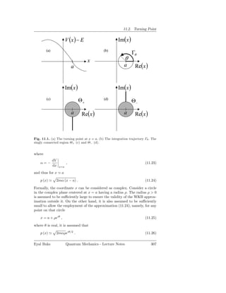
![Chapter 11. WKB Approximation
We consider below analytical continuation of the wavefunction given by Eq.
(11.21) for the case x > a into a region in the complex plane. Such a region
must excludes the vicinity of the turning point x = a where the WKB approx-
imation breaks down and in addition it is required to be singly connected to
allow analytical continuation. Two such regions are considered below, the first
one, which is labeled as Θ+ (see Fig. 11.1 (c)), excludes the circle |x − a| ≤ ρ
and also excludes the negative imaginary line x = a − ib, whereas the sec-
ond one, which is labeled as Θ− (see Fig. 11.1 (d)), also excludes the circle
|x − a| ≤ ρ and in addition excludes the positive imaginary line x = a + ib,
where in both cases the parameter b is assumed to be real and positive.
To perform the tailoring it is convenient to define the term
i
I± (θ) = ± dx′ p ,
Γθ
where the integration trajectory Γθ [see Fig. 11.1 (b)] contains two sections,
the first along the real axis from x = a to x = a + ρ and the second along the
′
arc x = a + ρeiθ from θ′ = 0 to θ ′ = θ. With the help of the approximation
(11.26) one finds that
ρ
√ θ
i 2mα ′
I± (θ) = ± dρ′ ρ′ + iρ3/2 dθ′ ei3θ /2
0 0
√ 3
2i e 2 iθ − 1
i 2mα 2 3/2
=± ρ − iρ3/2
3 3
√
2i 2mαρ3/2 3 iθ
=± e2
√ 3
2 2mαρ3/2 i(π(1∓ 1 )+ 3 θ)
= e 2 2 ,
3
(11.27)
thus
√
2 2mαρ3/2
I± (π) = ± , (11.28)
√ 3 3/2
2 2mαρ
I± (−π) = ∓ . (11.29)
3
The last result allows expressing the analytical continuation of the wavefunc-
tion given by Eq. (11.21) for the case x > a and evaluate its value at the
point x = a − ρ. For the case where the singly connected region Θ+ (Θ− ) is
employed, this is done using integration along the trajectory Γπ (Γ−π ), and
the result is labeled as ψ+ (a − ρ) [ψ− (a − ρ)]
Eyal Buks Quantum Mechanics - Lecture Notes 308](https://image.slidesharecdn.com/qmlecturenotes-130118222159-phpapp01/85/Quantum-Mechanics-Lecture-notes-318-320.jpg)
![11.2. Turning Point
√ √
2 2mαρ3/2 2mαρ3/2
C+ exp 3 + C− exp − 2 3
ψ+ (a − ρ) = 1/4 iπ/4
, (11.30)
(2mαρ) e
√ √
2mαρ3/2 2 2mαρ3/2
C+ exp − 2 3 + C− exp 3
ψ− (a − ρ) = . (11.31)
(2mαρ)1/4 e−iπ/4
Note that the denominators of Eqs. (11.30) and (11.31) are evaluated by
√
analytical continuation of the factor p [see Eq. (11.26)] along the trajectories
Γπ and Γ−π respectively. On the other hand, according to Eq. (11.21) in the
region x < a one finds by integration along the real axis that
√ 3
C 2 2mαρ 2
ψ (a − ρ) = exp − . (11.32)
(2mαρ)1/4 3
Comparing Eqs. (11.30) and (11.31) with Eq. (11.32) shows that for each of
the two choices Θ+ and Θ− the analytical continuation yields one exponential
term having the same form as the one in Eq. (11.32), and another one, which
diverges in the limit x → −∞. Excluding the diverging terms one finds that
continuity of the non diverging term requires that
C+ C−
C= = iπ/4 , (11.33)
e−iπ/4 e
and thus the tailored wavefunction is given by
x
√ exp 1 dx′ |p| x < a
C
|p|
ψ (x) = a . (11.34)
x
√
2C cos 1 dx′ p − π x > a
p 4
a
The fact that analytical continuation of the wavefunction in the region x < a
along the trajectory Γπ (Γ−π ) yields only the right to left (left to right) prop-
agating term in the region x > a, and the other term is getting lost along the
way, can be attributed to the limited accuracy of the WKB approximation.
As can be seen from Eq. (11.27), along the integration trajectory Γθ near the
point θ = ±π/3 one term becomes exponentially larger than the other, and
consequently, within the accuracy of this approximation the small term gets
lost.
It is important to keep in mind that the above result (11.34) is obtained
by assuming a particular form for the solution in the region x < a, namely
by assuming that in the classically forbidden region the coefficient of the
exponentially diverging term vanishes. This tailoring role will be employed in
the next section that deals with bound states in a classically accessible region
between two turning points [see Fig. 11.2(a)]. On the other hand, a modified
tailoring role will be needed when dealing with quantum tunneling. For this
case, which will be discussed below, we seek a wave function having the form
Eyal Buks Quantum Mechanics - Lecture Notes 309](https://image.slidesharecdn.com/qmlecturenotes-130118222159-phpapp01/85/Quantum-Mechanics-Lecture-notes-319-320.jpg)
![Chapter 11. WKB Approximation
V (x ) − E V (x ) − E
(a) (b)
x x
a b a b
Fig. 11.2. The region a ≤ x ≤ b bounded by the two turning points at x = a
and x = b is classically accessible in panel (a), whereas it is classically forbidden in
panel (b) .
x x
√+ exp
C 1 C
dx′ |p| + √− exp − 1 dx′ |p| x<a
|p| |p|
ψ (x) = a a . (11.35)
x
C i iπ
√
p exp dx′ p + 4 x>a
a
Thus, in this case only the term describing propagation from left to right
is kept in the region x > a, and the coefficient of the other term in that
region that describes propagation in the opposite direction is assumed to
vanish. Using the same tailoring technique as in the previous case one find
that C+ = 0 and C− = C, and thus
x
√ exp − 1 dx′ |p| x < a
C
|p|
ψ (x) = a . (11.36)
x
√
C exp i dx′ p + iπ x > a
p 4
a
11.3 Bohr-Sommerfeld Quantization Rule
Consider a classical accessible region a ≤ x ≤ b bounded by two turning
points at x = a and x = b, namely, consider the case where E > V (x) for
a ≤ x ≤ b and where E < V (x) for x < a and for x > b [see Fig. 11.2(a)].
We seek a normalizable solution, thus the wave function in the classically
forbidden regions x < a and for x > b is assumed to vanish in the limit
x → ±∞. Employing the tailoring role (11.34) with respect to the turning
point at x = a yields the following wave function for the region a ≤ x ≤ b
x
2Ca 1 π
ψa (x) = √ cos dx′ p − , (11.37)
p 4
a
Eyal Buks Quantum Mechanics - Lecture Notes 310](https://image.slidesharecdn.com/qmlecturenotes-130118222159-phpapp01/85/Quantum-Mechanics-Lecture-notes-320-320.jpg)
![Chapter 11. WKB Approximation
The Bohr-Sommerfeld quantization rule (11.40) can be used to relate the
classical time period T with the energy spacing ∆E = En+1 − En between
consecutive quantum eigen energies. As can be seen from the validity condi-
tion of the WKB approximation (11.13), the integer n is required to be large
to ensure the validity of Eq. (11.40). In this limit ∆E ≪ E, and thus by
taking the derivative of Eq. (11.40) with respect to energy one finds that
−1
∂E
∆E dx′ = 2π . (11.45)
∂p
In classical mechanics ∂E/∂p is the velocity of the particle v, therefor
−1
∂E
dx′ =T , (11.46)
∂p
thus
2π
∆E = . (11.47)
T
11.4 Tunneling
In this case we consider a classical forbidden region a ≤ x ≤ b bounded by
two turning points at x = a and x = b, namely, it is assumed that E < V (x)
for a ≤ x ≤ b and E > V (x) for x < a and for x > b [see Fig. 11.2(b)].
In classical mechanics a particle cannot penetrate into the potential barrier
in the region a ≤ x ≤ b, however such a process is possible in quantum
mechanics. Consider a solution having the form
x x
1
√ exp i
dx′ p + √p exp − i dx′ p
r
x<a
p
a a
x x
C+ C−
ψ (x) = √|p| exp 1 dx′ |p| + √|p| exp − 1 dx′ |p| a ≤ x ≤ b ,
b b
x
t
√ exp i ′ iπ
p dx p + 4 x>b
b
where we have introduced the transmission and reflection coefficients t and
r respectively. Such a solution describes an incident wave of unit amplitude
propagating in the region x < a from left to right, a reflected wave having
amplitude r in the same region, and a transmitted wave having amplitude t
in the opposite side of the barrier x > b.
Employing the tailoring role (11.36) yields C+ = 0 and C− = t. Moreover,
employing the tailoring role (11.34) and using the identity
x
x
1 1
exp − dx′ |p| = τ −1/2 exp − dx′ |p| , (11.48)
b a
Eyal Buks Quantum Mechanics - Lecture Notes 312](https://image.slidesharecdn.com/qmlecturenotes-130118222159-phpapp01/85/Quantum-Mechanics-Lecture-notes-322-320.jpg)
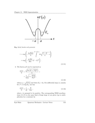
![Chapter 11. WKB Approximation
2 2
Moreover, current conservation requires that |t| + |r| = 1, thus
πE 2
|t|2 + −ite− E0 =1, (11.61)
2
and therefor the transmission probability τ = |t| is given by
1
τ= 2πE . (11.62)
1 + e− E0
As we have seen above, the analytical continuation of the transmitted
term in the region x → ∞ leads to the reflected term in the region
x → −∞. What about the incident term in the region x → −∞ (the first
term)? Note that this term (the incident one) becomes exponentially
small compared with the reflected term in a section near θ = 3π/4 along
the upper semicircle [due to the exponential factors exp ±ix2 /2x2 ]. 0
Consequently, within the accuracy of the WKB approximation it does
not contribute to the analytically continued value.
3. Consider one of the single-well eigenenergies En . The associated eigen-
state corresponding to the left well is labeled as |n, L and the one corre-
sponding to the right well as |n, R . The effect of finite penetrability of
the barrier can be evaluated using time independent perturbation theory
for the degenerate case [see Eq. (9.38]. For the unperturbed case, where
the barrier separating the two wells can be considered as impenetrable,
the level En is doubly degenerate, and the corresponding eigen space
is spanned by the vectors {|n, L , |n, R }. The projection of the Hamil-
tonian of the system H = p2 /2m + V on this eigen space is represented
by the 2 × 2 matrix Hn , which is given by
n, L| H |n, L n, L| H |n, R
Hn = . (11.63)
n, R| H |n, L n, R| H |n, R
Employing the approximations
H |n, L ≃ En |n, L , (11.64)
H |n, R ≃ En |n, R , (11.65)
one finds that
1 γ
Hn = En , (11.66)
γ∗ 1
where
γ = n, L |n, R , (11.67)
or in the coordinate representation
Eyal Buks Quantum Mechanics - Lecture Notes 316](https://image.slidesharecdn.com/qmlecturenotes-130118222159-phpapp01/85/Quantum-Mechanics-Lecture-notes-326-320.jpg)
![11.6. Solutions
∞
γ= dx ϕ∗ (x) ϕn,R (x) ,
n,L (11.68)
−∞
where ϕn,L (x) and ϕn,R (x) are the wavefunctions of the states |n, L
and |n, R respectively, i.e.
ϕn,L (x) = x |n, L , (11.69)
ϕn,R (x) = x |n, R . (11.70)
The main contribution to the overlap integral (11.68) comes from the
classically forbidden region |x| ≤ a, where x = ±a are turning points
(i.e., En = V (a) = V (−a)). With the help of Eq. (11.36) one finds that
x a
a |C|2 exp − 1 dx′ |p| exp − 1 dx′ |p|
−a x
γ≃ dx (11.71)
|p|
−a
a
a
1 dx
= |C|2 exp − ′
dx |p| , (11.72)
|p|
−a −a
(11.73)
where C is the normalization factor of the WKB wavefunction, which is
approximately given by C = 2 m/T (T is the time period of classical
oscillations of a particle having energy En in a well) in the limit of large
n [see Eq. (11.44)], thus
a
dx
4 |p/m|
a
−a 1
γ≃ exp − dx′ |p| . (11.74)
T
−a
Finally, By diagonalizing the matrix Hn one finds that the two eigenen-
ergies are En (1 ± γ).
4. The radial equation for the case of hydrogen is given by [see Eq. (7.61)]
− 2 d2
+ Veff (r) ukl (r) = Ekl ukl (r) , (11.75)
2µ dr2
where µ ≃ me is the reduced mass (me is the electron’s mass), and where
e2 l (l + 1) 2
Veff (r) = − + . (11.76)
r 2µr2
The eigenenergies Ekl are calculated using the Bohr-Sommerfeld quanti-
zation rule (11.40)
Eyal Buks Quantum Mechanics - Lecture Notes 317](https://image.slidesharecdn.com/qmlecturenotes-130118222159-phpapp01/85/Quantum-Mechanics-Lecture-notes-327-320.jpg)

![12. Path Integration
In this chapter, which is mainly based on Ref. [4], the technique of Feynman’s
path integration is briefly reviewed.
12.1 Charged Particle in Electromagnetic Field
Consider a point particle having mass m and charge q moving under the
influence of electric field E and magnetic field B, which are related to the
scalar potential ϕ and to the vector potential A by
1 ∂A
E = −∇ϕ − , (12.1)
c ∂t
and
B=∇×A. (12.2)
The classical Lagrangian of the system is given by Eq. (1.43)
1 q
L = m˙ 2 − qϕ + A · r ,
r ˙ (12.3)
2 c
and the classical Hamiltonian is given by Eq. (1.62)
2
p− q A
c
H= + qϕ . (12.4)
2m
The solution of the Euler Lagrange equations (1.8) yields the classical equa-
tion of motion of the system, which is given by Eq. (1.60)
1
m¨ = q E + r × B
r ˙ . (12.5)
c
In what follows, we consider for simplicity the case where both ϕ and A are
time independent. For this case H becomes time independent, and thus the
quantum dynamics is governed by the time evolution operator, which is given
by Eq. (4.9)](https://image.slidesharecdn.com/qmlecturenotes-130118222159-phpapp01/85/Quantum-Mechanics-Lecture-notes-331-320.jpg)
![Chapter 12. Path Integration
iHt
u (t) = exp − . (12.6)
The propagator K (r′ , t; r′ ) is defined by
b a
K (r′ , t; r′ ) = r′ | u (t) |r′ ,
b a b a (12.7)
where |r′ denotes a common eigenvector of the position operators x, y, and z
with vector of eigenvalues r′ = (x′ , y′ , z ′ ). As can be seen from the definition,
the absolute value squared of the propagator K (r′ , t; r′ ) is the probability
b a
density to find the particle at point r′ at time t given that it was initially
b
localized at point r′ at time t = 0.
a
Dividing the time interval (0, t) into N sections of equal duration allows
expressing the time evolution operator as
N
t
u (t) = u . (12.8)
N
The identity operator in the position representation [see Eq. (3.65)] is given
by
1r = d3 r′ |r′ r′ | . (12.9)
Inserting 1r between any two factors in Eq. (12.8) and using the notation
r′ = r′ ,
a 0 (12.10)
r′ = r′ ,
b N (12.11)
t
ǫ= , (12.12)
N
one finds that
K (r′ , t; r′ ) = r′ | u (ǫ) u (ǫ) u (ǫ) × · · · × u (ǫ) |r′
b a N 0
= d3 r′
1 d3 r′ × · · · ×
2 d3 r′
N−1
× r′ | u (ǫ) r′
N N−1 r′ ′
N−1 u (ǫ) rN−2 r′ ′ ′ ′
N−2 u (ǫ) × · · · × |r1 r1 | u (ǫ) |r0 ,
(12.13)
thus
N−1 N−1
K (r′ , t; r′ ) =
b a d3 r′
n K r′ ′
m+1 , ǫ; rm . (12.14)
n=1 m=0
In what follows the limit N → ∞ will be taken, and therefor it is sufficient
to calculate the infinitesimal propagator K r′ ′
m+1 , ǫ; rm to first order only
in ǫ.
Eyal Buks Quantum Mechanics - Lecture Notes 322](https://image.slidesharecdn.com/qmlecturenotes-130118222159-phpapp01/85/Quantum-Mechanics-Lecture-notes-332-320.jpg)
![Chapter 12. Path Integration
In the next step the identity operator in the momentum representation [see
Eq. (3.71)], which is given by
1p = d3 p′ |p′ p′ | , (12.22)
is inserted to the left of the ket vector |r′ . With the help of Eq. (3.75),
m
which is given by
1 ip′ · r′
r′ |p′ = exp , (12.23)
(2π )3/2
one finds that
ǫ
r′
m+1 exp −i p · r′ |r′
m
m
1 ip′ · r′ ′
m+1 − rm ǫ ′ ′
= d3 p′ exp exp −i p ·r .
(2π )3 m
(12.24)
Thus, by using Eq. (3.84), which is given by
1 ip′ · r′
d3 p′ exp = δ (r′ ) , (12.25)
(2π )3
one finds that
ǫ ǫ ′
r′
m+1 exp −i p · r′ |r′ = δ r′
m
′
m+1 − rm − r , (12.26)
m m
and thus
m 3/2 iǫ
K r′ ′
m+1 , ǫ; rm = exp Lm + O ǫ3/2 , (12.27)
2πiǫ
where
r′ ′ 2
m+1 −rm
m q A (r′ ) + A r′ ′ ′
ǫ m m+1 rm+1 − rm
Lm = −qϕ (r′ )+
m · . (12.28)
2 c 2 ǫ
Comparing Eq. (12.28) with the classical Lagrangian of the system, which
is given by Eq. (1.43)
1 q
L = m˙ 2 − qϕ + A · r ,
r ˙ (12.29)
2 c
shows that Lm is nothing but the Lagrangian at point r′
m
Eyal Buks Quantum Mechanics - Lecture Notes 324](https://image.slidesharecdn.com/qmlecturenotes-130118222159-phpapp01/85/Quantum-Mechanics-Lecture-notes-334-320.jpg)
![12.2. Classical Limit
Lm = L (r′ ) .
m (12.30)
As we have discussed above, the terms of order ǫ3/2 in Eq. (12.27) are not
expected to contribute to K (r′ , t; r′ ) in the limit of N → ∞. By ignoring
b a
these terms Eq. (12.14) becomes
N/2 N−1 N−1
Nm i t
K (r′ , t; r′ )
b a = lim d3 r′ exp
n L (r′ )
m .
N→∞ 2πit n=1
N m=0
(12.31)
Recall that the action in classical physics [see Eq. (1.4)] associated with a
given path is given by
S= dt L . (12.32)
Thus, by defining the integral operator
r′ N/2 N−1
b Nm
D [r′ (t)] = lim d3 r′ ,
n (12.33)
r′
a
N→∞ 2πit n=1
the propagator K (r′ , t; r′ ) can be written as
b a
r′
b i
K (r′ , t; r′ )
b a = D [r′ (t′ )] exp Sr′ (t′ ) , (12.34)
r′
a
where
t
Sr′ (t) = dt L [r′ (t)] . (12.35)
0
Equation (12.34), which is known as Feynman’s path integral, expresses the
propagator K (r′ , t; r′ ) in terms of all possible paths r′ (t′ ) satisfying r′ (0) =
b a
r′ and r′ (t) = r′ , where each path r′ (t′ ) contributes a phase factor given by
a b
exp iSr′ (t′ ) / , where Sr′ (t′ ) is the classical action of the path r′ (t′ ).
A note regarding notation: In the above derivation of Eq. (12.34) eigenval-
ues and eigenvectors were denoted with prime (e.g., r′ , |r′ , r′ |, p′ ) to make
them distinguishable from the corresponding operators (e.g., r and p). This
distinction is no longer needed for the rest of this chapter, since no quan-
tum operators are used to evaluate path integrals, and therefore, to make the
notation less cumbersome, we omit the prime notation.
12.2 Classical Limit
Recall that the Hamilton’s principle of least action states that the path taken
by a classical system is the one for which the action S obtains a local mini-
mum. This implies that for any infinitesimal change in the path the resultant
Eyal Buks Quantum Mechanics - Lecture Notes 325](https://image.slidesharecdn.com/qmlecturenotes-130118222159-phpapp01/85/Quantum-Mechanics-Lecture-notes-335-320.jpg)
![12.3. Aharonov-Bohm Effect
t
1 2 q
S= dt m˙ − qϕ + A · r
r ˙ . (12.37)
2 c
0
Consider first the case where the vector potential vanishes, i.e. A = 0. For
this case, the system is said to be conservative, and therefor, as we have seen
in chapter 1 [see Eq. (1.29)], the energy of the system
1
E = m˙ 2 + qϕ
r (12.38)
2
is a constant of the motion (see exercise 5 below). In terms of E the action
S (12.37), which is labeled as S0 for this case where A = 0, can be expressed
as
t
1 2
S0 = dt m˙ − qϕ
r
2
0
t
= dt −E + m˙ 2
r
0
rb
= −Et + m dr · r .
˙
ra
(12.39)
where ra = r (0) and rb = r (t). Employing Eq. (12.38) again allows rewriting
S0 as
rb
S0 = −Et + dr p (r) , (12.40)
ra
where p (r) is the local classical momentum
p (r) = 2m (E − qϕ (r)) . (12.41)
The phase factor in the path integral corresponding to S0 is given by
r
b
iS0 iEt i
exp = exp − exp dr p (r) . (12.42)
ra
Note the similarity between the second factor in the above equation and
between the WKB wavefunction [see Eq. (11.17)]. In the general case, where
A can be nonzero, the phase factor in the path integral becomes [see Eq.
(12.37)]
rb
iS iS0 iq
exp = exp exp dr · A . (12.43)
c
ra
Eyal Buks Quantum Mechanics - Lecture Notes 327](https://image.slidesharecdn.com/qmlecturenotes-130118222159-phpapp01/85/Quantum-Mechanics-Lecture-notes-337-320.jpg)
![Chapter 12. Path Integration
collector
rb , t
impenetrable
long coil
B≠0
ra ,0
source
Fig. 12.1. Two-slit interference experiment with a very long impenetrable cylinder
placed near the gap between the slits.
12.3.1 Two-slit Interference
Consider a two-slit interference experiment where electrons having charge
q = e are injected from a point source at ra (see Fig. 12.1). A collector at
point rb measures the probability density to detect an electron at that point.
A very long impenetrable cylinder is placed near the gap between the slits in
order to produce a magnetic field inside the cylinder in the direction normal
to the plane of the figure. The field outside the cylinder, however, can be
made arbitrarily small, and in what follows we assume that it vanishes.
The probability density Pb to detect the electron at time t by the collector
located at point rb is given by
Pb = |K (rb , t; ra )|2 , (12.44)
where the propagator (12.34) is given for this case by
rb
iS0,r(t) ie
K (rb , t; ra ) = D [r (t)] exp exp dr · A , (12.45)
ra c
r(t)
where the trajectories r (t) satisfy r (0) = ra and r (t) = rb .
How Pb is modified when the magnetic field is turned on, and consequently
the last factor in Eq. (12.45) starts to play a role? To answer this question
it is convenient to divide the sum over all paths into two groups, one for all
Eyal Buks Quantum Mechanics - Lecture Notes 328](https://image.slidesharecdn.com/qmlecturenotes-130118222159-phpapp01/85/Quantum-Mechanics-Lecture-notes-338-320.jpg)
![12.3. Aharonov-Bohm Effect
paths going through the left slit, and another for all paths going through the
right one. Here we disregard paths crossing a slit more than one time, as their
contribution is expected to be small. In general, the difference Θ12 between
the vector potential phase factor in Eq. (12.45) associated with two different
paths r1 (t) and r2 (t) is given by
e
Θ12 = dr · A− dr · A
c
r1 (t) r2 (t)
e
= dr · A ,
c
(12.46)
where the closed path integral is evaluated along the path r1 (t) in the forward
direction from ra to rb , and then along the path r2 (t) in the backward
direction from rb back to ra . This integral can be calculated using Stokes’
theorem [see Eq. (12.2)]
e e φ
Θ12 = dr · A = ds · B = 2π , (12.47)
c c φ0
where φ is the magnetic flux threaded through the area enclosed by the closed
path, and where
hc
φ0 = (12.48)
e
is the so called flux quantum. While Θ12 vanishes for pairs of paths going
through the same slit, it has the same value Θ12 = 2πφ/φ0 (Θ12 = −2πφ/φ0 )
for all the pairs where r1 (t) goes through the left (right) path and where r2 (t)
goes through the right (left) one. Thus, we come to the somewhat surprising
conclusion that the probability density Pb is expected to be dependent on
the magnetic field. The expected dependence is periodic in the magnetic
flux φ with flux quantum φ0 period. Such dependence cannot be classically
understood, since in this example the electrons can never enter the region in
which the magnetic field B is finite, and thus the Lorentz force vanishes in
the entire region accessible for the electrons outside the impenetrable coil.
12.3.2 Gauge Invariance
Consider the following gauge transformation
˜
A → A = A + ∇χ , (12.49)
ϕ→ϕ=ϕ,
˜ (12.50)
where χ = χ (r) is an arbitrary smooth and continuous function of r, which
is assumed to be time independent. As can be seen from Eqs. (12.1) and
Eyal Buks Quantum Mechanics - Lecture Notes 329](https://image.slidesharecdn.com/qmlecturenotes-130118222159-phpapp01/85/Quantum-Mechanics-Lecture-notes-339-320.jpg)
![Chapter 12. Path Integration
(12.2), this transformation leaves E and B unchanged, since ∇× (∇χ) = 0.
In chapter 1 we have seen that such a gauge transformation [see Eqs. (1.44)
and 1.45)] modifies the Lagrangian [see Eq. (1.43)]
˜ q
L → L = L + ∇χ · r , ˙ (12.51)
c
and also the action [see Eq. (12.37)]
t
˜ q
S →S=S+ dt ∇χ · r
˙
c
0
rb
q
= S+ dr · ∇χ
c
ra
q
= S + [χ (rb ) − χ (ra )] ,
c
(12.52)
however, the classical motion is unaffected.
In quantum mechanics, the propagator is expressed as a path integral
[see Eq. (12.34)], where each path r (t) contributes a phase factor given by
exp iSr(t) / . As can be seen from Eq. (12.52), this phase factor is generally
not singly determined, since it depends on the chosen gauge. This result,
however, should not be considered as paradoxical, since only phase difference
between different paths has any physical meaning. Indeed, as we have seen
above [see Eq. (12.47)], phase difference Θ12 , which determines the relative
phase between two different paths, is evaluated along a closed path, which is
singly determined, and therefore gauge invariant.
Exercise 12.3.1. Given that the wavefunction ψ (r′ , t′ ) solves the Schrödinger
equation with vector A and scalar ϕ potentials, show that the wavefunction
˜
ψ (r′ , t′ ), which is given by
˜ iqχ (r′ )
ψ (r′ , t′ ) = exp ψ (r′ , t′ ) , (12.53)
c
˜
solves the Schrödinger equation with vector A = A + ∇χ and scalar ϕ = ϕ
˜
potentials.
Solution 12.3.1. Using Eq. (3.76) one finds that
iqχ iqχ
exp − p exp
c c
iqχ iqχ
= exp − p, exp +p
c c
q∇χ
= p+ .
c
(12.54)
Eyal Buks Quantum Mechanics - Lecture Notes 330](https://image.slidesharecdn.com/qmlecturenotes-130118222159-phpapp01/85/Quantum-Mechanics-Lecture-notes-340-320.jpg)
![12.4. One Dimensional Path Integrals
This result implies that
iqχ q q iqχ q
exp − p− A− ∇χ exp = p− A , (12.55)
c c c c c
and therefore the following holds
iqχ ˜ iqχ
exp − H exp =H, (12.56)
c c
where [see Eq. (1.62)]
2
p− q A
c
H= + qϕ (12.57)
2m
is the Hamiltonian corresponding to the vector potential A, whereas
2
˜ p− q A− q ∇χ
c c
H= + qϕ , (12.58)
2m
˜
is the Hamiltonian corresponding to the vector potential A. Thus, one finds
that the state vector
˜ iqχ
ψ = exp |ψ (12.59)
c
˜
solves the Schrödinger equation with H, provided that the state vector |ψ
solves the Schrödinger equation with H, and therefore
˜ iqχ (r′ )
ψ (r′ , t′ ) = exp ψ (r′ , t′ ) . (12.60)
c
12.4 One Dimensional Path Integrals
Consider a point particle having mass m moving in one dimension along the
x axis under the influence of the potential V (x). The path integral (12.34)
for this case becomes
N/2 N−1 N−1
Nm i t xm+1 − xm
K (xb , t; xa ) = lim dxn exp L xm , t .
N→∞ 2πit n=1
N m=0 N
(12.61)
where the Lagrangian is
1
L (x, x) =
˙ mx2 − V (x) .
˙ (12.62)
2
Eyal Buks Quantum Mechanics - Lecture Notes 331](https://image.slidesharecdn.com/qmlecturenotes-130118222159-phpapp01/85/Quantum-Mechanics-Lecture-notes-341-320.jpg)

![12.4. One Dimensional Path Integrals
Employing the coordinate transformation (12.78) and the expansion of S
around the classical path allows rewriting the path integral (12.61) as
K (xb , t; xa ) = Pc (xb , t; xa ) K (t) , (12.85)
where
iSc
Pc (xb , t; xa ) = exp , (12.86)
i
K (t) = D [δ (t′ )] exp S2 + O δ 3 , (12.87)
and where
N/2 N−1
Nm
D [δ (t′ )] = lim dδ n . (12.88)
N→∞ 2πit n=1
The term K (t) is evaluated by integrating over all paths δ (t′ ) satisfying the
boundary conditions δ (0) = δ (t) = 0.
Exercise 12.4.2. Show that
dx′ Pc (xb , t2 ; x′ ) Pc (x′ , t1 ; xa ) K (t1 + t2 )
= . (12.89)
Pc (xb , t1 + t2 ; xa ) K (t1 ) K (t2 )
Solution 12.4.2. As can be seen from the definition of the propagator
(12.7), the following holds
dx′ K (xb , t2 ; x′ ) K (x′ , t1 ; xa ) = dx′ xb | u (t2 ) |x′ x′ | u (t1 ) |xa
= xb | u (t1 + t2 ) |xa
= K (xb , t1 + t2 ; xa ) .
(12.90)
Requiring that this property is satisfied by the propagator K (xb , t; xa ) that
is given by Eq. (12.85) leads to
dx′ Pc (xb , t2 ; x′ ) Pc (x′ , t1 ; xa ) K (t1 + t2 )
= . (12.91)
Pc (xb , t1 + t2 ; xa ) K (t1 ) K (t2 )
12.4.3 One Dimensional Harmonic Oscillator
For this case the Lagrangian is taken to be given by
mx2 mω 1 xx mω 2 x2
˙ ˙
L (x, x) =
˙ + − , (12.92)
2 2 2
Eyal Buks Quantum Mechanics - Lecture Notes 335](https://image.slidesharecdn.com/qmlecturenotes-130118222159-phpapp01/85/Quantum-Mechanics-Lecture-notes-345-320.jpg)

![12.5. Semiclassical Limit
mω
K (xb , t; xa ) = eAt
2πi sin (ωt)
i mω ωt mω 1 x2 − x2
× exp (xa − xb )2 cot (ωt) − 2xa xb tan + b a
.
2 2 4
(12.113)
In addition we require that in the limit ω, ω 1 → 0 the above result will
approach the result given by Eq. (12.65) for the propagator of a free particle.
This requirement yields A = 0. Note that
ωt 2xa xb
(xa − xb )2 cot (ωt) − 2xa xb tan = x2 + x2 cot (ωt) −
a b .
2 sin (ωt)
(12.114)
For the case ω 1 = 0 the propagator K (xb , t; xa ) becomes
mω
K (xb , t; xa ) =
2πi sin (ωt)
imω
× exp x2 + x2 cos (ωt) − 2xa xb
a b .
2 sin (ωt)
(12.115)
As can be seen from Eq. (12.103), the following holds
d2 Sc mω
=− , (12.116)
dxa dxb sin (ωt)
thus, similar to the case of a free particle [see Eq. (12.77)], also for the present
case of a harmonic oscillator, the propagator can be expressed in terms of
the classical action Sc as
i d2 Sc i
K (xb , t; xa ) = exp Sc . (12.117)
2π dxa dxb
12.5 Semiclassical Limit
In the semiclassical limit the Plank’s constant is considered to be small.
In this limit the dominant contribution to the path integral comes only from
paths near the classical one, which has the least action. This implies that in
the expansion of S around the classical path (12.80) terms of order O δ 3
can be approximately neglected. Thus, as can be seen from Eq. (12.87), in
this limit [see also Eq. (12.85)] the propagator K (xb , t; xa ) is evaluated by
path integration over the quadratic terms S2 only of the action [see Eq.
Eyal Buks Quantum Mechanics - Lecture Notes 339](https://image.slidesharecdn.com/qmlecturenotes-130118222159-phpapp01/85/Quantum-Mechanics-Lecture-notes-349-320.jpg)
![Chapter 12. Path Integration
(12.83)]. In the previous section we have exactly calculated the propagator
associated with the quadratic Lagrangian of a harmonic oscillator. The result
was expressed in Eq. (12.117) in terms of the classical action Sc . As can be
seen from Eq. (12.77), the same expression is applicable also for the case
of a free particle. It can be shown that the same form is also applicable
for expressing the propagator K (xb , t; xa ) in the semiclassical limit for the
general case
i d2 Sc i
K (xb , t; xa ) = exp Sc . (12.118)
2π dxa dxb
The proof of the above result, which requires generalization of the derivation
that led to Eq. (12.117) for the case of a general quadratic Lagrangian, will
not be given here. Another important result, which also is given here without
a proof, generalizes Eq. (12.118) for the case of motion in n spacial dimensions
i d2 Sc i
K (rb , t; ra ) = det exp Sc . (12.119)
2π dra drb
12.6 Problems
1. Show that
eǫ(A+B) = eǫA eǫB + O ǫ2 , (12.120)
where A and B are operators.
2. Show that
eǫ(A+B) = eǫB/2 eǫA eǫB/2 + O ǫ3 , (12.121)
where A and B are operators.
3. Show that
iǫV2 1 ir′2 ǫ
exp − = 3/2
d3 r′ exp −i V · r′ , (12.122)
2m (2πi) 2 m
where V is a vector operator.
4. Show that the energy (12.38) is indeed a constant of the motion.
5. Consider a quantum system having time independent Hamiltonian H and
a discrete energy spectrum. Express its partition function Z in terms of
the systems’s propagator K (xb , t; xa ).
6. Consider a one dimensional harmonic oscillator having mass m and res-
onance angular frequency ω in thermal equilibrium at temperature T .
Calculate the matrix elements x′′ | ρ |x′ of the density operator in the
basis of eigenvectors |x′ of the position operator x.
Eyal Buks Quantum Mechanics - Lecture Notes 340](https://image.slidesharecdn.com/qmlecturenotes-130118222159-phpapp01/85/Quantum-Mechanics-Lecture-notes-350-320.jpg)

![12.7. Solutions
Taking xb = xa and integrating over xa yields
∞
iEn t
dxa K (xa , t; xa ) = exp − . (12.140)
−∞ n
Thus, the partition function Z, which is given by Eq. (8.41)
Z= e−βEn , (12.141)
n
where β = 1/kB T , can be expressed as
∞
Z= dx′ K (x′ , −i β; x′ ) . (12.142)
−∞
6. Using Eq. (8.42) one finds that
x′′ | e−βH |x′
x′′ | ρ |x′ = , (12.143)
Z
where the partition function Z = Tr e−βH can be expressed in terms
of the propagator K (x′′ , t; x′ ) [see Eq. (12.142)]
∞
Z= dx′ K (x′ , −i β; x′ ) . (12.144)
−∞
Furthermore, as can be seen from the definition of the propagator [see
Eq. (12.7)]
iHt
K (x′′ , t; x′ ) = x′′ | e− |x′ , (12.145)
the following holds
x′′ | e−βH |x′ = K (x′′ , −i β; x′ ) . (12.146)
Thus, with the help of Eq. (12.115) one finds for the case of a harmonic
oscillator that (recall that sin (ix) = i sinh x and cos (ix) = cosh x)
∞
Z= dx′ K (x′ , −i β; x′ )
−∞
∞
mω mω [cosh (β ω) − 1] x′2
= dx′ exp −
2π sinh (β ω) −∞ sinh (β ω)
1
=
2 [cosh (β ω) − 1]
1
= ,
2 sinh βℏω
2
(12.147)
Eyal Buks Quantum Mechanics - Lecture Notes 343](https://image.slidesharecdn.com/qmlecturenotes-130118222159-phpapp01/85/Quantum-Mechanics-Lecture-notes-353-320.jpg)
![12.7. Solutions
x0 = . (12.169)
mω
b) Initially at time t = 0 the wavefunction ψ (x′ ) is given by [see Eq.
(5.108)]
2
1 1 x′′
ψ (x′′ , t = 0) = 1/2
exp − , (12.170)
π 1/4 x0 2 x0
where
x0 = . (12.171)
mω
The wave function at time t is evaluated using the propagator
∞
ψ (x′ , t) = dx′′ K (x′ , t; x′′ ) ψ (x′′ , 0)
−∞
1 1 1
=
x0 2πiωt π1/4 x1/2
0
8 2 ′′ 2 ′′ ′ ′ 2
i 3 xt +(x ) +2(2xt −x )(x −xt )+(x −xt )
∞ 2
x′′
−1
× dx′′ e ωt 2x2
0
2 x0
−∞
8 x2 +4x (x′ −x )+(x′ −x )2
i 3 t t t t
2x2
1 1 e ωt 0
= 1/2
x0 2πiωt π1/4 x0
′′ 2
∞ (1− ωt )( x 0 )
i
x −ix′′ (x′ −xt )
′′ − 2 +
ωtx2
× dx e 0 .
−∞
(12.172)
With the help of the identity
∞
1 1 4a
b2
√ exp −ax2 + bx dx = e , (12.173)
π a
−∞
one finds that
2 8 ix2 +4ix (x′ −x )
x′ −xt t t t
−1 1
+ 3
2 1+iωt x0 2ωtx2
e 0
ψ (x′ , t) = 1/2 √
. (12.174)
π 1/4 x0 1 + iωt
The probability density f (x′ ) = |ψ (x′ , t)|2 to find the particle near
point x′ at time t is thus given by
x′ −xt 2
1
−
e 1+(ωt)2 x0
f (x′ ) = √ , (12.175)
πx0 1 + (ωt)2
Eyal Buks Quantum Mechanics - Lecture Notes 347](https://image.slidesharecdn.com/qmlecturenotes-130118222159-phpapp01/85/Quantum-Mechanics-Lecture-notes-357-320.jpg)
![13. Adiabatic Approximation
The adiabatic approximation can be employed for treating systems having
slowly varying Hamiltonian. This chapter is mainly based on Ref. [5].
13.1 Momentary Diagonalization
The Schrödinger equation (4.1) is given by
d |α
i = H |α . (13.1)
dt
For any given value of the time t the Hamiltonian H (t) is assumed to have
a discrete spectrum
H (t) |n (t) = En (t) |n (t) , (13.2)
where n = 1, 2, · · · , the momentary eigenenergies En (t) are real, and the set
of momentary eigenvectors is assumed to be orthonormal
n (t) |m (t) = δ nm . (13.3)
The general solution can be expanded using the momentary eigenvectors as
a momentary basis
|α (t) = an (t) eiβ n (t) |n (t) . (13.4)
n
The phase factors β n (t) in the expansion (13.4) are chosen to be given by
β n (t) = ξ n (t) + γ n (t) , (13.5)
where the phase factors
t
1
ξ n (t) = − dt′ En (t′ ) (13.6)
are the so-called dynamical phases, and the other phase factors](https://image.slidesharecdn.com/qmlecturenotes-130118222159-phpapp01/85/Quantum-Mechanics-Lecture-notes-359-320.jpg)

![13.3. Adiabatic Limit
Exercise 13.1.2. Show that for n = m the following holds
˙
m (t)| H |n (t)
m (t) |n (t) =
˙ . (13.14)
En (t) − Em (t)
Solution 13.1.2. Taking the time derivative of Eq. (13.2)
˙ ˙ ˙
H |n + H |n = En |n + En |n ,
˙ (13.15)
and the inner product with m (t)|, where m = n, yields the desired identity.
13.2 Gauge Transformation
The momentary orthonormal basis {|n (t′ ) }n , which is made of eigenvec-
tors of H (t), is clearly not singly determined. Consider the following ‘gauge
transformation’ [see for comparison Eq. (12.49)]
|n (t′ ) → |˜ (t′ ) = e−iΛ(t ) |n (t′ ) ,
′
n (13.16)
where Λ (t′ ) is arbitrary real function of time. The geometrical phase γ n (t),
which is given by Eq. (13.7)
t
γ n (t) = i dt′ n (t′ ) |n (t′ ) ,
˙ (13.17)
t0
is transferred to
γ n (t) → γ n (t) = γ n (t) + Λ (t) − Λ (t0 ) .
˜ (13.18)
Thus, in general the geometrical phase is not singly determined. However, it
becomes singly determined, and thus gauge invariant, if the path is closed,
namely if H (t) = H (t0 ), since for such a case Λ (t) = Λ (t0 ).
13.3 Adiabatic Limit
In the adiabatic limit the terms m (t) |n (t) are considered to be negligibly
˙
small. As can be seen from Eq. (13.14), this limit corresponds to the case
where the rate of change in time of the Hamiltonian approaches zero. In
this limit the coefficients an (t) become constants [see Eq. (13.13)], and the
solution (13.4) thus becomes
|α (t) = an eiβn (t) |n (t) . (13.19)
n
Eyal Buks Quantum Mechanics - Lecture Notes 351](https://image.slidesharecdn.com/qmlecturenotes-130118222159-phpapp01/85/Quantum-Mechanics-Lecture-notes-361-320.jpg)
![Chapter 13. Adiabatic Approximation
13.4 The Case of Two Dimensional Hilbert Space
In this case the Hilbert space is two dimensional and the Hamiltonian can be
represented by a 2 × 2 matrix, which is conveniently expressed as a combina-
tion of Pauli matrices
H=h0 I + h · σ ,
˙ (13.20)
where I is the 2 × 2 identity matrix, h0 is a real scalar, h = (h1 , h2 , h3 ) is a
three-dimensional real vector, and the components of the Pauli matrix vector
σ are given by
01 0 −i 1 0
σ1 = , σ2 = , σ3 = . (13.21)
10 i 0 0 −1
√
ˆ
Using the notation h = H h, where H = ˆ
h · h, and where h is a unit vector,
given in spherical coordinates by
ˆ
h = (cos ϕ sin θ, sin ϕ sin θ, cos θ) , (13.22)
one finds that
cos θ sin θ exp (−iϕ)
H=h0 I + H
˙ . (13.23)
sin θ exp (iϕ) − cos θ
The orthonormal eigenvectors are chosen to be given by [see Eqs. (6.199) and
(6.200)]
cos θ exp − iϕ
2 2
|+ =
˙ , (13.24)
sin θ exp iϕ
2 2
− sin θ exp − iϕ
2 2
|− =
˙ , (13.25)
cos θ exp iϕ
2 2
and the following holds +|+ = −|− = 1, +|− = 0, and
H |± = (h0 ± H) |± . (13.26)
Note that the eigenstates |± are independent of both h0 and H.
The geometrical phase (13.7) can be evaluated by integration along the
path h (t)
t h(t)
γ n (t) = i dt′ n (t′ ) |n (t′ ) = i
˙ dh · n (h)| ∇h |n (h) . (13.27)
0 h(0)
Exercise 13.4.1. Show that
iˆ
ϕ
±| ∇h |± = ∓ ctg θ . (13.28)
2H
Eyal Buks Quantum Mechanics - Lecture Notes 352](https://image.slidesharecdn.com/qmlecturenotes-130118222159-phpapp01/85/Quantum-Mechanics-Lecture-notes-362-320.jpg)

![Chapter 13. Adiabatic Approximation
13.6 Slow and Fast Coordinates
Consider a system whose Hamiltonian is given by
H = H0 + H1 . (13.66)
The Hamiltonian H0 is assume to depend on a set of coordinates x = ¯
(x1 , x2,... ) and on their canonically conjugate variables p = (p1 , p2,... ), i.e.
¯
H0 = H0 (¯, p). In what follows the coordinates x = (x1 , x2,... ) will be con-
x ¯ ¯
sidered as slow, and thus H0 will be considered as the Hamiltonian of the
slow subsystem. The other part of the system is a fast subsystem, which is
assumed to have a much faster dynamics and its energy spectrum is assumed
to be discrete. The Hamiltonian of the fast subsystem H1 is assumed to para-
metrically depend on the slow degrees of freedom x, i.e. H1 = H1 (¯). This
¯ x
dependence gives rise to the coupling between the slow and fast subsystems.
An adiabatic approximation can be employed in order to simplify the
equations of motion of the combined system. In what follows, for simplicity,
this method will be demonstrated for the case where the slow subsystem is
assumed to be composed of a set of decoupled harmonic oscillators. For this
case the Hamiltonian H0 is taken to be given by
p2
l ml ω 2 x2
l l
H0 = + , (13.67)
2ml 2
l
where ml and ωl are the mass and angular frequency of mode l, respectively.
The Hamiltonian of the fast subsystem H1 (¯), which depends paramet-
x
rically on x, has a set of eigenvectors and corresponding eigenvalues for any
¯
given value of x
¯
H1 |n (¯) = εn (¯) |n (¯) ,
x x x (13.68)
where n = 1, 2, · · · . The set of ’local’ eigenvectors {|n (¯) } is assumed to
x
form an orthonormal basis of the Hilbert space of the fast subsystem, and
thus the following is assumed to hold
m (¯) |n (¯) = δ mn ,
x x (13.69)
and [see Eq. (2.23)]
|k (¯) k (¯)| = 1F ,
x x (13.70)
k
where 1F is the identity operator on the Hilbert space of the fast subsystem.
The state of the entire system ψ (t) at time t is expanded at any point x
¯
using the ’local’ basis {|n (¯) }
x
ψ (t) = ξ n (¯, t) |n (¯) .
x x (13.71)
n
Eyal Buks Quantum Mechanics - Lecture Notes 358](https://image.slidesharecdn.com/qmlecturenotes-130118222159-phpapp01/85/Quantum-Mechanics-Lecture-notes-368-320.jpg)
![13.6. Slow and Fast Coordinates
In the above expression a mixed notation is being employed. On one hand,
the ket notation is used to denote the state of the fast subsystem (the terms
|n (¯) ). On the other hand, a wavefunction in the position representation
x
(the terms ξ n (¯, t)) is employed to denote the state of the slow subsystem.
x
Substituting the expansion (13.71) into the Schrödinger equation (4.1)
dψ
i = Hψ , (13.72)
dt
leads to
[H0 + εn (¯)] ξ n (¯, t) |n (¯) = i
x x x ˙ x
ξ n (¯, t) |n (¯) ,
x (13.73)
n n
where overdot represents time derivative. Projecting m (¯)| leads to
x
x x x x x ˙ x
m (¯)| H0 ξ n (¯, t) |n (¯) + εm (¯) ξ m (¯, t) = i ξ m (¯, t) . (13.74)
n
By calculating the term [see Eq. (13.69)]
m (¯)| p2 ξ n (¯, t) |n (¯) = ξ n (¯, t) m (¯)| p2 |n (¯)
x l x x x x l x
+ 2 (pl ξ n (¯, t)) m (¯)| pl |n (¯) + δ mn p2 ξ n (¯, t) ,
x x x l x
(13.75)
introducing the notation
Am,n;l ≡ − m (¯)| pl |n (¯) ,
x x (13.76)
and using [see Eq. (13.70)]
m (¯)| p2 |n (¯) =
x l x m (¯)| pl |k (¯) k (¯)| pl |n (¯)
x x x x
k
= −pl Am,n;l + Am,k;l Ak,n;l , (13.77)
k
one obtains
m (¯)| p2 ξ n (¯, t) |n (¯)
x l x x
= ξ n (¯, t) −pl Am,n;l +
x Am,k;l Ak,n;l
k
− 2Am,n;l pl ξ n (¯, t) +
x δ mn p2 ξ n (¯, t) .
l x
(13.78)
With the help of Eqs. (13.67) and (13.74) one finds that
Eyal Buks Quantum Mechanics - Lecture Notes 359](https://image.slidesharecdn.com/qmlecturenotes-130118222159-phpapp01/85/Quantum-Mechanics-Lecture-notes-369-320.jpg)
![Chapter 13. Adiabatic Approximation
1
ξ n (¯, t) −pl Am,n;l +
x Am,k;l Ak,n;l
2ml n
l k
1
− −2Am,n;l pl ξ n (¯, t) + δ mn p2 ξ n (¯, t)
x l x
2ml n
l
ml ω 2 x2
l l ˙ x
+ ξ m (¯, t) + εm (¯) ξ m (¯, t) = i ξ m (¯, t) .
x x x
2
l
(13.79)
ˆ
Defining the matrices Al = Am,n;l , (ˆ)m,n = εm δ mn , and the vector
ε
m,n
˘
ξ = ξ n , the above can be written in a matrix form as
n
·
1 2 ml ω2 x2
ˆ
pl − Al + l l
+ˆ ˘ = i ˘ .
ε ξ ξ (13.80)
2ml 2
l
ˆ
To calculate the off-diagonal matrix elements of Al we apply pl to Eq.
(13.68) and project m (¯)|, where m = n
x
m (¯)| pl H1 |n (¯) = m (¯)| pl εn (¯) |n (¯) .
x x x x x (13.81)
∂
Using Eq. (13.69), the definition (13.76) and pl = −i ∂xl [see Eq. (3.29)] one
finds that [compare with Eq. (13.14)]
m (¯)| ∂Hl1 |n (¯)
x ∂x x
Am,n;l = i . (13.82)
εn − εm
ˆ
In the adiabatic approximation the off diagonal elements of Al [see Eq.
(13.82)] are considered as negligible small. In this case the set of equations
of motion (13.80) becomes decoupled
˙ (pl − Am,m;l (¯))2 ml ω2 x2
x l l
i ξm = + + εm (¯) ξ m .
x (13.83)
2ml 2
l
As can be seen from the above result (13.83), the adiabatic approximation
greatly simplifies the system’s equations of motion. The effect of the fast
subsystem on the dynamics of the slow one is taken into account by adding a
vector potential Am,m;l (¯) and a scalar potential εm (¯) to the Schrödinger
x x
equation of the slow subsystem [compare with Eq. (4.168)]. However, both
potential terms depend on the state m that is being occupied by the fast
subsystem.
Exercise 13.6.1. Show that if m (¯)| ∂/∂xl |m (¯) is pure real then
x x
Amm;l (¯) = 0 .
x (13.84)
Eyal Buks Quantum Mechanics - Lecture Notes 360](https://image.slidesharecdn.com/qmlecturenotes-130118222159-phpapp01/85/Quantum-Mechanics-Lecture-notes-370-320.jpg)
![13.8. Solutions
Solution 13.6.1. Note that in general the diagonal elements Am,m;l are real
since pl is Hermitian [see Eq. (13.76)]. On the other hand, if m (¯)| ∂/∂xl |m (¯)
x x
is pure real then Amm;l (¯) is pure imaginary, thus for this case Amm;l (¯) = 0.
x x
13.7 Problems
1. Consider the following ’gauge transformation’
cos θ exp − iϕ
2 2 ˜ ˙ cos θ
2
|+ =
˙ → + = , (13.85)
sin θ exp iϕ
2 2
θ
sin exp (iϕ)
2
− sin θ exp − iϕ
2 2 ˜ ˙ − sin θ
2
|− =
˙ → − = . (13.86)
cos θ exp iϕ
2 2
cos θ exp (iϕ)
2
Find an expression for the transformed geometrical phase γ ± (t).
˜
2. Consider a particle having mass m confined by a time dependent potential
well given by
0 if 0 ≤ x ≤ a
V (x) = . (13.87)
∞ if x < 0 or x > a
where the width of the well a oscillates in time according to
a (t) = a0 1 − α sin2 (ω p t) , (13.88)
where a0 , α and ω p are positive, and where α < 1.
a) Under what condition the adiabatic approximation is expected to be
valid.
b) Calculate the geometrical phases γ n [see Eq. (13.7)] for a cyclic evo-
lution from time t = 0 to time t = π/ω p .
13.8 Solutions
1. The following holds
iϕ
˜
+ = exp |+ , (13.89)
2
iϕ
˜
− = exp |− , (13.90)
2
thus the transformed geometrical phase γ ± (t) [see Eq. (13.18)] becomes
˜
ϕ (t) ϕ (t0 )
γ n (t) → γ n (t) = γ n (t) −
˜ + . (13.91)
2 2
Eyal Buks Quantum Mechanics - Lecture Notes 361](https://image.slidesharecdn.com/qmlecturenotes-130118222159-phpapp01/85/Quantum-Mechanics-Lecture-notes-371-320.jpg)
![Chapter 13. Adiabatic Approximation
2. The momentary eigenenergies of the system are given by
2 2 2
π n
En (t) = 2 , (13.92)
2ma2
0 1 − α sin2 (ω p t)
where n = 1, 2, · · · . The corresponding eigenvectors are denoted by
|n (t) .
a) In general, the main contribution to interstate transitions come from
time periods when the energy gap between neighboring eigenener-
gies is relatively small. At any given time the smallest energy gap
between momentary eigenenergies is the one between the two lowest
states H21 (t) = E2 (t) − E1 (t). Furthermore, the main contribution
to the transition probability is expected to come from the regions near
minima points of the energy gap H21 (t). Near the minima point at
time t = 0 the energy gap H21 (t) is given by
3 2π2
H21 (t) = 2
2ma2 1 − α sin2 (ω p t)
0
3 2 π2
= 1 + 2α (ωp t)2 + O t3
2ma2 0
3 2 π2
= 1 + 4α (ω p t)2 + O t3 .
2ma2 0
(13.93)
The estimated transition probability for the two dimensional case
is given by Eq. (13.65). In view of the fact that all other energy
gaps between momentary eigenenergies is at least 5/3 larger than
H21 , it is expected that this estimate is roughly valid for the present
case. The requirement that the transition probability given by Eq.
(13.65) is small is taken to be the validity condition for the adiabatic
approximation. Comparing the above expression for H21 (t) near t =
0 with Eq. (13.50) yields the following validity condition
3 π3
2ωp α1/2 ≪ . (13.94)
2ma2
0
b) In general, the term n (t′ ) |n (t′ ) is pure imaginary [see Eq. (13.9)].
˙
On the other hand, the fact that the wavefunctions of one dimensional
bound states can be chosen to be real (see exercise 7 of chapter 4),
implies that n (t′ ) |n (t′ ) is pure real. Thus n (t′ ) |n (t′ ) = 0 and
˙ ˙
therefore all geometrical phases vanish.
Eyal Buks Quantum Mechanics - Lecture Notes 362](https://image.slidesharecdn.com/qmlecturenotes-130118222159-phpapp01/85/Quantum-Mechanics-Lecture-notes-372-320.jpg)
![14. The Quantized Electromagnetic Field
This chapter discusses the quantization of electromagnetic (EM) field for the
relatively simple case of a free space cavity.
14.1 Classical Electromagnetic Cavity
Consider an empty volume surrounded by conductive walls having infinite
conductivity. The Maxwell’s equations (in Gaussian units) are given by
1 ∂E
∇×B = , (14.1)
c ∂t
1 ∂B
∇×E = − , (14.2)
c ∂t
∇·E = 0 , (14.3)
∇·B = 0 , (14.4)
where c = 2.99 × 10⁸ m s−1 is the speed of light in vacuum. In the Coulomb
gauge the vector potential A is chosen such that
∇·A =0 , (14.5)
and the scalar potential ϕ vanishes in the absence of sources (charge and
current). In this gauge both electric and magnetic fields E and B can be
expressed in terms of A only as [see Eqs. (1.41) and (1.42)]
1 ∂A
E=− , (14.6)
c ∂t
and
B=∇×A. (14.7)
Exercise 14.1.1. Show that
1 ∂2A
∇2 A = . (14.8)
c2 ∂t2](https://image.slidesharecdn.com/qmlecturenotes-130118222159-phpapp01/85/Quantum-Mechanics-Lecture-notes-373-320.jpg)
![14.1. Classical Electromagnetic Cavity
1 d2 q
q∇2 u = u . (14.20)
c2 dt2
Multiplying by an arbitrary unit vector n leads to
ˆ
∇2 u · n
ˆ 1 d2 q
= 2 . (14.21)
u·nˆ c q dt2
The left hand side of Eq. (14.21) is a function of r only while the right hand
side is a function of t only. Therefore, both should equal a constant, which is
denoted as −κ2 , thus
∇2 u+κ2 u = 0 , (14.22)
and
d2 q
+ω 2 q = 0 ,
κ (14.23)
dt2
where
ω κ = cκ . (14.24)
Exercise 14.1.3. Show that the general solution can be expanded as
A= qn (t) un (r) . (14.25)
n
where the set {un } forms a complete orthonormal basis spanning the vector
space of all solutions of Eq. (14.16) satisfying the proper boundary conditions
on the conductive walls having infinite conductivity.
Solution 14.1.3. Equation (14.16) should be solved with the boundary con-
ditions of a perfectly conductive surface. Namely, on the surface S enclosing
the cavity we have B · ˆ = 0 and E × ˆ = 0, where ˆ is a unit vector normal
s s s
to the surface. To satisfy the boundary condition for E we require that u be
normal to the surface, namely, u = ˆ (u · ˆ) on S. This condition guarantees
s s
also that the boundary condition for B is satisfied. To see this we calculate
the integral of the normal component of B over some arbitrary portion S ′ of
S. Using Eq. (14.7) and Stoke’s’ theorem one finds that
(B · ˆ) dS = q
s [(∇ × u) · ˆ] dS
s
S′ S′
=q u · dl ,
C
(14.26)
where the close curve C encloses the surface S ′ . Thus, since u is normal to
the surface, one finds that the integral along the close curve C vanishes, and
therefore
Eyal Buks Quantum Mechanics - Lecture Notes 365](https://image.slidesharecdn.com/qmlecturenotes-130118222159-phpapp01/85/Quantum-Mechanics-Lecture-notes-375-320.jpg)
![Chapter 14. The Quantized Electromagnetic Field
(B · ˆ) dS = 0 .
s (14.27)
S′
Since S ′ is arbitrary we conclude that B · ˆ =0 on S. Each solution of Eq.
s
(14.16) that satisfies the boundary conditions is called an eigen mode. As
can be seen from Eq. (14.23), the dynamics of a mode amplitude q is the
same as the dynamics of an harmonic oscillator having angular frequency
ω κ = cκ. Inner product between different solutions of Eq. (14.16) that satisfy
the boundary conditions can be defined as
u1 , u2 ≡ (u1 · u2 ) dV , (14.28)
V
where the integral is taken over the volume of the cavity. Using Eq. (14.16)
one finds that
κ2 − κ2
2 1 (u1 · u2 ) dV = u1 · ∇2 u2 − u2 · ∇2 u1 dV . (14.29)
V V
Using Green’s theorem one finds that
κ2 − κ2
2 1 (u1 · u2 ) dV = (u1 · [(ˆ · ∇) u2 ] − u2 · [(ˆ · ∇) u1 ]) dS .
s s
V S
(14.30)
Using Eq. (14.19), the boundary condition u = ˆ (u · ˆ) on S, and writing ∇ =
s s
ˆ (ˆ · ∇) − ˆ× (ˆ × ∇), we find that the right hand side of (14.30) vanishes.
s s s s
Thus, solutions with different κ2 are orthogonal to each other. Let {un } be a
complete orthonormal basis spanning the vector space of all solutions of Eq.
(14.16) satisfying the boundary conditions. For any two vectors in this basis
the orthonormality condition is
un , um = (un · um ) dV = δ n,m . (14.31)
V
Using such a basis we can expand the general solution as
A= qn (t) un (r) . (14.32)
n
Exercise 14.1.4. Show that the total electric energy in the cavity is given
by
1
UE = ˙2
qn , (14.33)
8πc2 n
and the total magnetic energy is given by
1
UB = κ2 qn .
n
2
(14.34)
8π n
Eyal Buks Quantum Mechanics - Lecture Notes 366](https://image.slidesharecdn.com/qmlecturenotes-130118222159-phpapp01/85/Quantum-Mechanics-Lecture-notes-376-320.jpg)
![14.1. Classical Electromagnetic Cavity
Solution 14.1.4. Using Eqs. (14.6),(14.7) and (14.25) one finds that the
fields are given by
1
E=− qn un ,
˙ (14.35)
c n
and
B= qn ∇ × un . (14.36)
n
The total energy of the field is given by UE + UB , where UE (UB ) is the
energy associated with the electric (magnetic) field, namely,
1
UE = E2 dV , (14.37)
8π V
and
1
UB = B2 dV . (14.38)
8π V
Using Eqs. (14.35) and (14.31) one finds that
1
UE = ˙2
qn , (14.39)
8πc2 n
and using Eq. (14.36) one finds that
1
UB = qn qm (∇ × un ) · (∇ × um ) dV . (14.40)
8π n,m V
The last integral can be calculated by using the vector identity
∇ · (F1 × F2 ) = (∇ × F1 ) · F2 − F1 · (∇ × F2 ) , (14.41)
applied to un × (∇ × um ), thus
(∇ × un )·(∇ × um ) = ∇·(un × (∇ × um ))+un ·[∇ × (∇ × um )] . (14.42)
Using the divergence theorem and the fact that un and (∇ × um ) are or-
thogonal to each other on S one finds that the volume integral of the first
term vanishes. To calculate the integral of the second term it is convenient
to use the identity
∇ × (∇ × um ) = ∇ (∇ · um ) − ∇2 um . (14.43)
This together with Eqs. (14.19), (14.16), and (14.31) lead to
1
UB = κ2 qn .
n
2
(14.44)
8π n
Eyal Buks Quantum Mechanics - Lecture Notes 367](https://image.slidesharecdn.com/qmlecturenotes-130118222159-phpapp01/85/Quantum-Mechanics-Lecture-notes-377-320.jpg)
![Chapter 14. The Quantized Electromagnetic Field
The Lagrangian of the system is given by [see Eq. (1.16)]
1 qn ω 2 qn
˙2 2
L = UE −UB = − n , (14.45)
4πc2 n
2 2
where the symbol overdot is used for derivative with respect to time, and
where ω n = cκn . The Euler-Lagrange equations, given by
d ∂L ∂L
− =0, (14.46)
dt ∂ qn
˙ ∂qn
lead to Eq. (14.23).
The variable canonically conjugate to qn is [see Eq. (1.20)]
∂L 1
pn = = qn .
˙ (14.47)
∂ qn
˙ 4πc2
The classical Hamiltonian HF of the field is given by [see Eq. (1.22)]
4πc2 p2
n 1 ω 2 qn
n
2
HF = pn qn − L =
˙ + . (14.48)
n n
2 4πc2 2
The Hamilton-Jacobi equations of motion, which are given by
∂HF
qn =
˙ = 4πc2 pn , (14.49)
∂pn
∂HF ω2
pn = −
˙ = − n2 qn , (14.50)
∂qn 4πc
lead also to Eq. (14.23). Note that, as expected, the following holds
HF = UE +UB , (14.51)
namely the Hamiltonian expresses the total energy of the system.
14.2 Quantum Electromagnetic Cavity
The coordinates qn and their canonically conjugate variables pn are regarded
as Hermitian operators satisfying the following commutation relations [see
Eqs. (3.5) and (4.41)]
[qn , pm ] = i δ n,m , (14.52)
and
[qn , qm ] = [pn , pm ] = 0 . (14.53)
Eyal Buks Quantum Mechanics - Lecture Notes 368](https://image.slidesharecdn.com/qmlecturenotes-130118222159-phpapp01/85/Quantum-Mechanics-Lecture-notes-378-320.jpg)
![14.2. Quantum Electromagnetic Cavity
In general, the Heisenberg equation of motion (4.37) of an operator A(H) is
given by
dA(H) 1 (H) ∂A(H)
= A(H) , HF + . (14.54)
dt i ∂t
Thus, with the help of Eq. (14.48) one finds that
qn = 4πc2 pn ,
˙ (14.55)
and
ω2
n
pn = −
˙ qn . (14.56)
4πc2
It is useful to introduce the annihilation and creation operators
ωn 4πic2 pn
an = eiωn t qn + , (14.57)
8πc2 ωn
ωn 4πic2 pn
a† = e−iωn t
n qn − . (14.58)
8πc2 ωn
The phase factor eiωn t in the definition of an is added in order to make it
time independent. The inverse transformation is given by
2πc2
qn = e−iωn t an + eiωn t a† ,
n (14.59)
ωn
ωn
pn = i −e−iωn t an + eiωn t a† .
n (14.60)
8πc2
The commutation relations for the these operators are derived directly from
Eqs. (14.52) and (14.53)
an , a† = δ n,m ,
m (14.61)
[an , am ] = a† , a† = 0 .
n m (14.62)
The Hamiltonian (14.48) can be expressed using Eqs. (14.59) and (14.60) as
1
HF = ω n a† an +
n . (14.63)
n
2
The eigenstates are the photon-number states |s1, s2 , ..., sn , ... , which satisfy
[see chapter 5]
1
HF |s1, s2 , · · · , sn , · · · = ωn sn + |s1, s2 , · · · , sn , · · · . (14.64)
n
2
The following holds [see Eqs. (5.28) and (5.29)]
Eyal Buks Quantum Mechanics - Lecture Notes 369](https://image.slidesharecdn.com/qmlecturenotes-130118222159-phpapp01/85/Quantum-Mechanics-Lecture-notes-379-320.jpg)
![Chapter 14. The Quantized Electromagnetic Field
√
an |s1, s2 , · · · , sn , · · · = sn |s1, s2 , · · · , sn − 1, · · · , (14.65)
√
a† |s1, s2 , · · · , sn , · · · = sn + 1 |s1, s2 , · · · , sn + 1, · · ·
n . (14.66)
The non-negative integer sn is the number of photons occupying mode n.
The vector potential A (14.25) becomes
2πc2
A (r, t) = e−iωn t an + eiωn t a† un (r) .
n (14.67)
n
ωn
14.3 Periodic Boundary Conditions
Consider the case where the EM field is confined to a finite volume V , which
for simplicity is taken to have a cube shape with edge L = V −1/3 . The
eigen modes and eigen frequencies of the EM field are found in exercise 1
of this chapter for the case where the walls of the cavity are assumed to
have infinite conductance [see Eq. (14.84)]. It is however more convenient to
assume instead periodic boundary conditions, since the spatial dependence
of the resulting eigen modes [denoted by un (r)], can be expressed in terms of
exponential functions, rather than trigonometric functions [see Eqs. (14.77),
(14.78) and (14.79)]. For this case Eq. (14.63) becomes
1
HF = ω k a† ak,λ +
k,λ , (14.68)
2
k,λ
and Eq. (14.67) becomes
2πc2
A (r, t) = ˆk,λ ei(k·r−ωk t) ak,λ + ˆ∗ e−i(k·r−ωk t) a†
ǫ ǫk,λ k,λ , (14.69)
ωk V
k,λ
where the eigen frequencies are given by ω k = c |k|. In the limit of large
volume the discrete sum over wave vectors k can be replaced by an integral
∞ ∞ ∞
V
→ 3 dkx dky dkz , (14.70)
k
(2π) −∞ −∞ −∞
and the commutation relations between field operators become
[ak,λ , ak′ ,λ ] = a† , a† ′ ,λ = 0 ,
k,λ k (14.71)
ak,λ , a† ′ ,λ′ = δ λ,λ′ δ k − k′ .
k (14.72)
The sum over λ contains two terms corresponding to two polarization
vectors ˆk,λ , which are normalized to unity and mutually orthogonal, i,e.
ǫ
ˆ∗ · ˆk,λ′ = δ λ,λ′ . Furthermore, the Coulomb gauge condition requires that
ǫk,λ ǫ
Eyal Buks Quantum Mechanics - Lecture Notes 370](https://image.slidesharecdn.com/qmlecturenotes-130118222159-phpapp01/85/Quantum-Mechanics-Lecture-notes-380-320.jpg)
![14.5. Solutions
finite for any ξ. Moreover, it is assumed that F (∞) → 0. In this case the
Euler-Maclaurin summation formula, which is given by
∞ ∞
1 1 ′ 1 ′′′
F (0) + F (n) − dN F (N) = − F (0) + F (0) + · · · ,
2 n=1 0 12 720
(14.96)
can be employed to evaluate U (d). The following holds
F ′ (ξ) = −2ξ 2 f ξ 2 , (14.97)
thus for small ξ [where the cutoff function is assumed to be given by
f (y) = 1] F ′′ (ξ) = −4ξ and F ′′′ (ξ) = −4, and therefore
π2 cL2
U (d) = − . (14.98)
720d3
The force per unit area (pressure) P (d) is found by taking the derivative
with respect to d and by dividing by the area L2
π2 c
P (d) = − . (14.99)
240d4
The minus sign indicates that the force is attractive.
3. The average energy U in thermal equilibrium is given by Eq. (8.332),
which is given by
∂ log Zc
U =− , (14.100)
∂β
where Zc = Tr e−βH is the canonical partition function, H is the
Hamiltonian [see Eq. (14.64)], β = 1/kB T and kB is the Boltzmann’s
constant. The partition function is found by summing over all photon-
number states |s1, s2 , ...
∞
Zc = s1, s2 , ...| e−βH |s1, s2 , ...
s1, s2 ,...=0
∞
ωn (sn + 1 )
= e−β n 2
s1, s2 ,...=0
∞
ωn (sn + 1 )
= e−β 2
n sn =0
1
= ,
n 2 sinh β ωn
2
(14.101)
Eyal Buks Quantum Mechanics - Lecture Notes 375](https://image.slidesharecdn.com/qmlecturenotes-130118222159-phpapp01/85/Quantum-Mechanics-Lecture-notes-385-320.jpg)

![Chapter 15. Light Matter Interaction
and the vector potential A is given by Eq. (14.69)
2πc2
A (r, t) = ˆk,λ ei(k·r−ωk t) ak,λ + ˆ∗ e−i(k·r−ωk t) a†
ǫ ǫk,λ k,λ . (15.5)
k,λ
ωk V
15.2 Transition Rates
While the Hamiltonian Hp is considered as a perturbation, the unperturbed
Hamiltonian is taken to be H0 + HF . The eigenvectors of H0 + HF are la-
beled as |{sk,λ } , η . While the integers sk,λ represent the number of photons
occupying each of the modes of the EM field, the index η labels the atomic
energy eigenstate. The following holds
H0 |{sk,λ } , η = Eη |{sk,λ } , η ,
where Eη is the energy of the atomic state, and
1
HF |{sk,λ } , η = ω k sk,λ + |{sk,λ } , η . (15.6)
2
k,λ
15.2.1 Spontaneous Emission
Consider the case where the system is initially in a state |i = |{sk,λ = 0} , ηi ,
for which all photon occupation numbers are zero, and the atomic state is la-
beled by the index ηi . The final state is taken to be |f = a† |{sk,λ = 0} , ηf ,
k,λ
for which one photon is created in mode k, λ, and the atomic state is labeled
by the index η f . To lowest nonvanishing order in perturbation theory the
transition rate wi,f is given by Eq. (10.34)
2π
wi,f = 2
δ (ω k − ωi,f ) | f| Hp |i |2 , (15.7)
where ω i,f = Eηi − Eηf / . With the help of Eqs. (14.69) and (15.3) wi,f
can be rewritten as
2
e 4π2 c2 2
wi,f = δ (ω k − ω i,f ) f| ˆ∗ · pe−ik·r a† |i
ǫk,λ k,λ . (15.8)
me c ωk V
As can be seen from Eq. (7.2), the following holds
1
[H0 , r] = (−i ) p , (15.9)
me
thus
Eyal Buks Quantum Mechanics - Lecture Notes 380](https://image.slidesharecdn.com/qmlecturenotes-130118222159-phpapp01/85/Quantum-Mechanics-Lecture-notes-390-320.jpg)

![15.2. Transition Rates
Exercise 15.2.1. Show that the selection rule for the magnetic quantum
number m is given by
∆m = mf − mi ∈ {−1, 0, 1} . (15.20)
Solution 15.2.1. Using the relations Lz = xpy − ypx and [xi , pj ] = i δ ij
it is easy to show that [Lz , z] = 0 and [Lz , x ± iy] = ± (x ± iy). The first
relation together with Eq. (15.19) imply that
0 = kf , lf , mf , σf | [Lz , z] |ki , li , mi , σi
= (mf − mi ) kf , lf , mf , σf | z |ki , li , mi , σi ,
(15.21)
whereas the second relation together with Eq. (15.19) imply that
kf , lf , mf , σ f | [Lz , x ± iy] |ki , li , mi , σ i
= (mf − mi ) kf , lf , mf , σf | x ± iy |ki , li , mi , σ i
= ± kf , lf , mf , σf | (x ± iy) |ki , li , mi , σ i ,
(15.22)
thus
(mf − mi ∓ 1) kf , lf , mf , σf | x ± iy |ki , li , mi , σi = 0 . (15.23)
Therefore Mi,f = 0 [see Eq. (15.16)] unless ∆m ∈ {−1, 0, 1}. The transition
∆m = 0 is associated with linear polarization in the z direction, whereas
the transitions ∆m = ±1 are associated with clockwise and counterclockwise
circular polarizations respectively.
Exercise 15.2.2. Show that the selection rule for the quantum number l is
given by
∆l = lf − li ∈ {−1, 1} . (15.24)
Solution 15.2.2. Using Eq. (15.40), which is given by
L2 , L2 , r =2 2
rL2 +L2 r , (15.25)
together with Eq. (15.18) yield
kf , lf , mf , σ f | L2 , L2 , r |ki , li , mi , σ i
4
=2 (lf (lf + 1) + li (li + 1)) kf , lf , mf , σ f | r |ki , li , mi , σ i
= 4
(lf (lf + 1) − li (li + 1))2 kf , lf , mf , σf | r |ki , li , mi , σ i ,
(15.26)
thus with the help of the identity
Eyal Buks Quantum Mechanics - Lecture Notes 383](https://image.slidesharecdn.com/qmlecturenotes-130118222159-phpapp01/85/Quantum-Mechanics-Lecture-notes-393-320.jpg)
![Chapter 15. Light Matter Interaction
2
(lf (lf + 1) − li (li + 1)) − 2 (lf (lf + 1) + li (li + 1))
2
= (li + lf ) (li + lf + 2) (li − lf ) − 1 ,
(15.27)
one finds that
(li + lf ) (li + lf + 2) (li − lf )2 − 1 kf , lf , mf , σf | r |ki , li , mi , σi = 0 . (15.28)
Since both li and lf are non negative integers, and consequently li +lf +2 > 0,
one finds that kf , lf , mf , σf | r |ki , li , mi , σ i can be nonzero only when li =
lf = 0 or |∆l| = 1. However, for the first possibility, for which li = mi = lf =
mf = 0, the wavefunctions of both states |ki , li , mi , σi and |kf , lf , mf , σ f is a
function of the radial coordinate r only [see Eq. (6.130)], and consequently
kf , lf , mf , σ f | r |ki , li , mi , σi = 0. Therefore the selection rule is given by ∆l ∈
{−1, 1}.
15.3 Semiclassical Case
Consider the case where one mode of the EM field, which has angular fre-
quency ω and polarization vector ˆ, is externally driven to a coherent state
ǫ
|α , where |α| ≫ 1. In the semiclassical approximation the annihilation op-
erator of the driven mode a is substituted by the complex constant α (and
the operator a† by α∗ ). Furthermore, all other modes are disregarded. When
ω is close to a specific transition frequency ω a = (E+ − E− ) / between two
atomic states, which are labeled by |+ and |− , the atom can be approxi-
mately considered to be a two level system. In the dipole approximation the
matrix element +| Hp |− is given by [see Eqs. (15.3), (15.9) and (15.16)]
+| Hp |− = e−iωt − ∗ iωt
e , (15.29)
2
where
2π
= −2ieω a αˆ · +| r |− .
ǫ (15.30)
ωV
It is convenient to express the complex frequency as = ω 1 e−iθ , where
both ω 1 and θ are real. The frequency ω1 is called the Rabi frequency. Due
to selection rules the diagonal matrix elements of Hp vanish.
The Schrödinger equation is given by
d
i |ψ = H |ψ , (15.31)
dt
where the matrix representation in the basis {|+ , |− } of the Hamiltonian
H is given by [see Eq. (15.29)]
Eyal Buks Quantum Mechanics - Lecture Notes 384](https://image.slidesharecdn.com/qmlecturenotes-130118222159-phpapp01/85/Quantum-Mechanics-Lecture-notes-394-320.jpg)
![15.3. Semiclassical Case
ωa ω1 e−i(ωt+θ) − ei(ωt+θ)
H=
˙ i(ωt+θ) −i(ωt+θ) . (15.32)
2 ω1 e −e −ω a
It is convenient to express the general solution as
iωt iωt
|ψ (t) = b+ (t) exp − |+ + b− (t) exp |− . (15.33)
2 2
Substituting into the Schrödinger equation yields [see Eq. (6.230)]
d b+ 1 ∆ω ω 1 e−iθ − ei(2ωt+θ) b+
i = iθ −i(2ωt+θ) ,
dt b− 2 ω1 e −e −∆ω b−
(15.34)
where
∆ω = ω a − ω . (15.35)
In the rotating wave approximation the rapidly oscillating terms e±i(2ωt+θ)
are disregarded, since their influence in the long time limit is typically neg-
ligible. This approximation is equivalent to the assumption that the second
term in Eq. (15.29) can be disregarded. Furthermore, the phase factor θ can
be eliminated by resetting the time zero point accordingly. Thus, the Hamil-
tonian can be taken to be given by
ω a ω1 e−iωt
H=
˙ , (15.36)
2 ω1 eiωt −ωa
and the equation of motion in the rotating frame can be taken to be given
by
d b+ 1 ∆ω ω1 b+
i = . (15.37)
dt b− 2 ω1 −∆ω b−
The time evolution is found using Eq. (6.138) [see also Eq. (6.234)]
b+ (t)
b− (t)
cos θ − i √∆ω sin θ −i √ ω21 sin θ b+ (0)
2 ω1 +(∆ω)2 ω1 +(∆ω)2
= ,
−i √ ω21 sin θ 2 cos θ + i √∆ω sin θ 2 b− (0)
ω1 +(∆ω) ω2 +(∆ω)
1
(15.38)
where
ω 2 + (∆ω)2 t
1
θ= . (15.39)
2
Eyal Buks Quantum Mechanics - Lecture Notes 385](https://image.slidesharecdn.com/qmlecturenotes-130118222159-phpapp01/85/Quantum-Mechanics-Lecture-notes-395-320.jpg)
![Chapter 15. Light Matter Interaction
15.4 Problems
1. Show that
L2 , L2 , r =2 2
rL2 +L2 r . (15.40)
2. Consider an atom having a set of orthonormal energy eigenstates {|ηn }.
The oscillator strength fnm associated with the transition between state
|ηn to state |ηm is defined by
2me ω n,m
fnm = | ηf | r |η i |2 . (15.41)
3
Show that
fn,n′ = 1 . (15.42)
n′
3. Calculate the lifetime of all states of hydrogen atom having principle
quantum number n = 2.
4. Consider a hydrogen atom that is initially at time t → −∞ in its ground
state. An electric field in the z direction given by
τ2
E (t) = E0ˆ
z , (15.43)
τ2 + t2
where τ is a constant having the dimension of time, is externally applied.
Calculate the probability p2p to find the atom in the sub-shell 2p at time
t → ∞.
5. Consider a particle having mass m and charge q moving in a one dimen-
sional harmonic oscillator having angular resonance frequency ω. Cal-
culate using the dipole approximation the rate of spontaneous emission
from the number state |n to the ground state |0 .
15.5 Solutions
1. Using the relations [Lx , z] = −i y, [Ly , z] = i x and [Lz , z] = 0 one finds
that
L2 , z = L2 , z + L2 , z
x y
= i (−Lx y − yLx + Ly x + xLy )
= i V·ˆ,z
(15.44)
where V = r × L − L × r. Thus the following holds L2 , r = i V. With
the help of the identities
Eyal Buks Quantum Mechanics - Lecture Notes 386](https://image.slidesharecdn.com/qmlecturenotes-130118222159-phpapp01/85/Quantum-Mechanics-Lecture-notes-396-320.jpg)
![15.5. Solutions
[Lx , Vz ] = −Lx [Lx , y] − [Lx , y] Lx + [Lx , Ly ] x + x [Lx , Ly ] = −i Vy ,
[Ly , Vz ] = − [Ly , Lx ] y − y [Ly , Lx ] + Ly [Ly , x] + [Ly , x] Ly = i Vx ,
[Lz , Vz ] = − [Lz , Lx y] − [Lz , yLx ] + [Lz , Ly x] + [Lz , xLy ] = 0 ,
one finds that
L2 , L2 , z =i L2 , Vz
2
= (Lx Vy + Vy Lx − Ly Vx − Vx Ly )
2
= (L × V − V × L) · ˆ ,
z
(15.45)
thus
L2 , L2 , r = 2
(L × V − V × L)
2
= (L× (r × L) − L× (L × r) − (r × L) ×L+ (L × r) ×L)
= 2 2 rL2 +L2 r .
(15.46)
2. Trivial by the Thomas-Reiche-Kuhn sum rule (4.66).
(se)
3. The rate of spontaneous emission Γi→f,λ in general is given by Eq. (15.14)
(se) αfs ω 3
i,f
Γi→f,λ = 4π |Mi,f |2 . (15.47)
2πc2
The transition frequency ω i,f between the levels n = 2 to n = 1 is given
by [see Eq. (7.66)]
me e4 1 1
ωi,f = − + , (15.48)
2 3 22 12
thus in terms of the Bohr’s radius a0 [see Eq. (7.64)] one has
2
(se) 33 α5 me c2 Mi,f
fs
Γi→f,λ = .
28 a0
The matrix element of z = r cos θ and of u± = 2−1/2 (x ± iy) =
2−1/2 r sin θe±iφ are given by [see Eq. (7.92)]
n′ , l′ , m′ | z |n, l, m
∞ 1 2π
′ ∗
3
= dr r Rn′ l′ Rnl d (cos θ) dφ cos θ Ylm
′ Ylm ,
0 −1 0
(15.49)
and
Eyal Buks Quantum Mechanics - Lecture Notes 387](https://image.slidesharecdn.com/qmlecturenotes-130118222159-phpapp01/85/Quantum-Mechanics-Lecture-notes-397-320.jpg)
![Chapter 15. Light Matter Interaction
n′ , l′ , m′ | u± |n, l, m
∞ 1 2π
1 ′ ∗
3
= dr r Rn′ l′ Rnl d (cos θ) dφ sin θe±iφ Ylm
′ Ylm ,
2
0 −1 0
(15.50)
where n, l and m are the quantum members of hydrogen’s energy eigen-
vectors. The final state is taken to be the ground state (n, l, m) = (1, 0, 0).
In the dipole approximation the transition (2, 0, 0) → (1, 0, 0) is forbidden
due to the selection rule ∆l ∈ {−1, 1}. Using the identities
3/2
1
R10 (r) = 2 e−r/a0 , (15.51)
a0
3/2
1 r
R20 (r) = (2 − r/a0 ) e− 2a0 , (15.52)
2a0
3/2
1 r r
R21 (r) = √ e− 2a0 , (15.53)
2a0 3a0
1
Y00 (θ, φ) = , (15.54)
4π
1 3
Y1−1 (θ, φ) = sin θe−iφ , (15.55)
2 2π
1 3
Y10 (θ, φ) = cos θ , (15.56)
2 π
1 3
Y11 (θ, φ) = − sin θeiφ , (15.57)
2 2π
where a0 is Bohr’s radius [see Eq. (7.64)], one finds for the radial part
that
∞ √
3 27 6
dr r R10 R21 = a0 , (15.58)
35
0
and for the angular part that
1 2π
∗ 1
d (cos θ) dφ cos θ Y00 Y10 = √ , (15.59)
3
−1 0
1 2π
∗
d (cos θ) dφ cos θ Y00 Y1±1 = 0 , (15.60)
−1 0
1 2π
∗
d (cos θ) dφ sin θe±iφ Y00 Y10 = 0 , (15.61)
−1 0
Eyal Buks Quantum Mechanics - Lecture Notes 388](https://image.slidesharecdn.com/qmlecturenotes-130118222159-phpapp01/85/Quantum-Mechanics-Lecture-notes-398-320.jpg)
![Chapter 15. Light Matter Interaction
thus with the help of the residue theorem one finds that
∞ 3EI ′ τ
dt′ ei 4 t = πe− . (15.71)
−∞ τ 2 + t′2
The matrix element 2, 1, m| z |1, 0, 0 is calculated with the help of Eq.
(15.49)
∞ 1 2π
2, 1, m| z |1, 0, 0 = 3
dr r R21 R10 d (cos θ) dφ cos θ (Y1m )∗ Y00
0 −1 0
√
27 2a0
= δ m,0 ,
35
(15.72)
where
2
a0 = (15.73)
µe2
is the Bohr’s radius, thus
2
215 eE0 a0 τ 3EI τ
p2pm = π e− 2 δ m,0 . (15.74)
310
5. The oscillator is assumed to move along the z direction. The rate of
(se)
spontaneous emission Γ|n →|0 ,λ with polarization λ into solid angle d
is given in the dipole approximation by [see Eqs. (15.14) and (15.16)]
(se) q 2 (nω)3 2
dΓ|n →|0 ,λ = | 0| z |n |2 ˆ∗ · ˆ
ǫk,λ z d , (15.75)
2π c3
where ˆ∗ is the polarization unit vector. With the help of Eqs. (5.11),
ǫk,λ
(5.28) and (5.29) one finds that
(se) q 2 (nω)3 n 2
dΓ|n →|0 ,λ = δ n,1 ˆ∗ · ˆ
ǫk,λ z d . (15.76)
2π c3 2mω
Integrating over d in spherical coordinates θ and φ with the help of the
relation
π 1
4π
d cos2 θ = dφ d (cos θ) cos2 θ = , (15.77)
−π −1 3
and summing over the two orthogonal polarization yields the total rate
of spontaneous emission
(se) 2q 2 ω2
Γ|n →|0 = δ n,1 . (15.78)
3mc3
Eyal Buks Quantum Mechanics - Lecture Notes 390](https://image.slidesharecdn.com/qmlecturenotes-130118222159-phpapp01/85/Quantum-Mechanics-Lecture-notes-400-320.jpg)
![16. Identical Particles
This chapter reviews the identical particles postulate of quantum mechanics
and second quantization formalism. It is mainly based on the first chapter of
Ref. [6].
16.1 Basis for the Hilbert Space
Consider a system containing some integer number N of identical particles.
For the single particle case, where N = 1, the state of the system |α can be
expanded using an orthonormal basis {|ai }i that spans the single particle
Hilbert space. Based on the single particle basis {|ai }i we wish to construct
a basis for the Hilbert space of the system for the general case, where N can
be any integer. This can be done in two different ways, depending on whether
the identical particles are considered to be distinguishable or indistinguishable
(see example in Fig. 16.1).
Suppose that the particles can be labelled by numbers as billiard balls.
In this approach the particles are considered as distinguishable. For this case
a basis for the Hilbert space of the many-particle system can be constructed
from all vectors having the form |1 : i1 , 2 : i2 , · · · , N : iN . The ket vector
|1 : i1 , 2 : i2 , · · · , N : iN represents a state having N particles, where the
particle that is labelled by the number m (m = 1, 2, · · · , N ) is in the single
particle state |aim . Each ket vector |1 : i1 , 2 : i2 , · · · , N : iN can be char-
acterized by a vector of occupation numbers n = (n1 , n2 , · · · ), where ni is
¯
the number of particles occupying the single particle state |ai . Let gn be ¯
the number of different ket-vectors having the form |1 : i1 , 2 : i2 , · · · , N : iN
that are characterized by the same vector of occupation numbers n. It is easy
¯
to s](https://image.slidesharecdn.com/qmlecturenotes-130118222159-phpapp01/85/Quantum-Mechanics-Lecture-notes-401-320.jpg)