
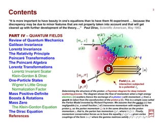
![“A poet once said, ‘The whole universe is in a glass of wine.’ We will probably never know in what sense
he meant that, for poets do not write to be understood. But it is true that if we look at a glass of wine
closely enough we see the entire universe. There are the things of physics: the twisting liquid which
evaporates depending on the wind and weather, the reflections in the glass, and our imagination adds the
atoms. The glass is a distillation of the earth’s rocks, and in its composition we see the secrets of the
universe’s age, and the evolution of stars. What strange array of chemicals are in the wine? How did they
come to be? There are the ferments, the enzymes, the substrates, and the products. There in wine is
found the great generalization: all life is fermentation. Nobody can discover the chemistry of wine without
discovering, as did Louis Pasteur, the cause of much disease. How vivid is the claret, pressing its
existence into the consciousness that watches it! If our small minds, for some convenience, divide this
glass of wine, this universe, into parts – physics, biology, geology, astronomy, psychology, and so on –
remember that nature does not know it! So let us put it all back together, not forgetting ultimately what it
is for. Let it give us one more final pleasure: drink it and forget it all! ”
Richard Feynman
Epicatechin
TARTARIC ACID (C4H6O6)
2,3-dihydroxybutanedioic acid
Tartaric acid is, from a winemaking
perspective, the most important in wine
due to the prominent role it plays in
maintaining the chemical stability of the
wine and its color and finally in influencing
the taste of the finished wine. [Wikipedia]
MALIC ACID (C4H6O5)
hydroxybutanedioic acid
Malic acid, along with tartaric acid, is one of the
principal organic acids found in wine grapes. In
the grape vine, malic acid is involved in several
processes which are essential for the health
and sustainability of the vine. [Wikipedia]
CITRIC ACID (C6H8O7)
2-hydroxypropane-1,2,3-tricarboxylic acid
The citric acid most commonly found in wine
is commercially produced acid supplements
derived from fermenting sucrose solutions.
[Wikipedia]
Three primary acids are found in wine grapes:
RESVERATROL DERIVATIVES
trans cis
Malvidin-3-glucoeide
Procyanidin B1 Quercetin
R = H; resueratrol
R = glucose; p Ice Id
TYPICAL WINE FLAVONOIDS
Resveratrol (3,5,4'-trihydroxy-
trans-stilbene) is a stilbenoid,
a type of natural phenol, and
a phytoalexin produced
naturally by several plants.
[Wikipedia]
In red wine, up to 90% of the
wine's phenolic content falls
under the classification of
flavonoids. These phenols,
mainly derived from the
stems, seeds and skins are
often leached out of the
grape during the maceration
period of winemaking. These
compounds contribute to the
astringency, color and
mouthfeel of the wine.
[Wikipedia]
Prolog
2](https://image.slidesharecdn.com/linked-inslides-qft-130507130813-phpapp02/85/Part-IV-Quantum-Fields-2-320.jpg)
![2017
MRT
PART V – THE HYDROGEN ATOM
What happens at 10−−−−10 m?
The Hydrogen Atom
Spin-Orbit Coupling
Other Interactions
Magnetic & Electric Fields
Hyperfine Interactions
Multi-Electron Atoms and Molecules
Appendix - Interactions
The Harmonic Oscillator
Electromagnetic Interactions
Quantization of the Radiation Field
Transition Probabilities
Einstein’s Coefficients
Planck’s Law
A Note on Line Broadening
The Photoelectric Effect
Higher Order Electromagnetic Interactions
References
“Quantum field theory is the way it is because […] this is the only way to reconcile the principles of
quantum mechanics […] with those of special relativity. […] The reason that quantum field theory
describes physics at accessible energies is that any relativistic quantum theory will look at sufficiently
low energy like a quantum field theory.” Steven Weinberg, Preface to The Quantum Theory of Fields, Vol. I.
PART III – QUANTUM MECHANICS
Introduction
Symmetries and Probabilities
Angular Momentum
Quantum Behavior
Postulates
Quantum Angular Momentum
Spherical Harmonics
Spin Angular Momentum
Total Angular Momentum
Momentum Coupling
General Propagator
Free Particle Propagator
Wave Packets
Non-Relativistic Particle
Appendix: Why Quantum?
References
4](https://image.slidesharecdn.com/linked-inslides-qft-130507130813-phpapp02/85/Part-IV-Quantum-Fields-4-320.jpg)


;( θθθθµµµµ
xf
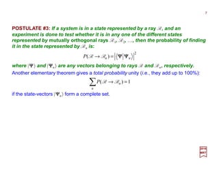
so that the state vector |ψ 〉 will transform according to (i.e., by using Taylor’s expansion):
As an example of symmetry,consideratransformation (parametrizedbythevariableθ,
e.g., an angle ϕ,a translation a or aLorentzboostζ )onthespace-timecoordinates xµ :
in which the real infinitesimal is ε =dθ and the generator for the parameter θ is given by:
∑= =
∂
∂
∂
∂
−=
3
0 0
);(
)(
µ
µ
θ
µ
θ
θ
θ
x
xf
iT
all
ψεεψθψ
θ
θ
θψ
ψ
θ
θ
θψψψψψψ
µµ
µ
µ
θ
µ
µ
µ
µ
µ
θ
µ
µµ
µ
µ
µµµµµ
)]([)()()(
);(
)(
)(
);(
)()()()()(
2
0
0
OTixTdix
x
xf
idix
x
x
xf
dxx
x
dxxxdxx
T
++=+=
∂
∂
∂
∂
−+=
∂
∂
∂
∂
+≡
∂
∂
+≈+=→
∑
∑∑
=
=
111
44444 344444 21
)(Generator
all
all
2017
MRT
11](https://image.slidesharecdn.com/linked-inslides-qft-130507130813-phpapp02/85/Part-IV-Quantum-Fields-11-320.jpg)
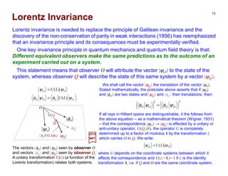
![with f a(θ ,θ) a function of the θs and θs. Taking θ a =0 as the coordinate of the identity,
we must have:
)),(()()( θθθθ fTTT =
aaa
ff θθθ == ),0()0,(
As mentionned above, the transformation of such continuous groups must be represen-
ted on the physical Hilbert space by unitary operators U[T(θ )]. For a Lie group these op-
erators can be represented by a power series (e.g., in the neighborhoodof the identity):
A finite set of real continuous parameters θ a describe a group of transformations T(θ )
with each element of the group connected to the identity by a path (i.e., UU−1=1) within
the group. The group multiplication law U(T2)U(T1)=U(T2T1) thus takes on the form
(i.e., a connected Lie group):
According to f a(θ ,0)= f a(0 ,θ)=θ a above, the expansion of f a(θ ,θ) to second-order must
take the form:
2017
MRT
K+++= ∑∑∑ c b
bc
cb
a
a
a
TTiTU θθθθ
2
1
)]([ 1
where Ta, Tbc =Tcb, &c. are Hermitian operators independent of the θ s. Suppose that the
U[T(θ )] form an ordinary (i.e., φ =0) representation of this group of transformations, i.e.:
))],(([)]([)]([ θθθθ fTUTUTU =
...),( +⊕+= ∑∑c b
cba
bc
aaa
ff θθθθθθ
with real coefficients f a
bc. The addition of the second-order term is emphasized by ⊕.
12](https://image.slidesharecdn.com/linked-inslides-qft-130507130813-phpapp02/85/Part-IV-Quantum-Fields-12-320.jpg)
![(The Σ were also omitted to get space.) The terms of order 1, θ, θ, and θ 2 automatically
match on both sides of this equation – from the θ θ terms we get a non-trivial condition:
KKKK ++++++++=+++×+++ bc
ccbb
a
cba
bc
aa
bc
cb
a
a
bc
cb
a
a
TTfiTTitti ))(()(][][ 2
1
2
1
2
1 θθθθθθθθθθθθθθ 111
∑−−=
a
a
a
bccbbc TfiTTT
Since we are following Weinberg’s development, he points out that: This shows that if
we are given the structure of the group, i.e., the function f a(θ,θ ), and hence its quadratic
coefficient f a
bc, we can calculate the second-order terms (i.e., Tbc) in U[T(θ)] from the
generators Ta appearing in the first-order terms. (A pretty amazing fact wouldn’t you say?)
Applying the multiplication rule U[T(θ)]U[T(θ)]=U[T( f (θ ,θ )] and using the series
U[T(θ)]=1+iθ a Ta +½θ bθ c Tbc +…above withθ → f a (θ,θ)=θ a +θ a + f a
bc θ b θ c ,we get:
where Ca
bc are a set of real constants known as structure constants:
∑=−≡
a
a
a
bcbccbcb TCiTTTTTT ],[
2017
MRT
However, as he points out: There is a consistency condition: the operator Tbc, must be
symmetricinbandc(becauseitisthesecondderivativeof U[T(θ)]withrespect toθ b andθ c)
so the equation Tbc =−Tb Tc −iΣa f a
bc Ta above requires that the commutation relations be:
a
cb
a
bc
a
bc ffC +−=
Such a set of commutation relations is known as a Lie algebra to mathematicians.
13](https://image.slidesharecdn.com/linked-inslides-qft-130507130813-phpapp02/85/Part-IV-Quantum-Fields-13-320.jpg)
![This is the case for instance for ‘translations’ in spacetime, or for ‘rotations’ about any
one fixed axis(though not both together).Then the coefficients f a
bc in the function f a(θ,θ )
=θ a +θ a +Σbc f a
bc θ b θ c vanish,and so do the structure constants Ca
bc=− f a
bc+ f a
cb, that is
Ca
bc =0. So, [Tb ,Tc]≡TbTc −TcTb reduces to the fact that the generators then all commute:
aaa
f θθθθ +=),(
N
N
TUTU
=
θ
θ)]([
Such a group is called Abelian. In this case, it is easy to calculate U[T(θ)] for all θ a.
Again, from the group multiplication rule U[T(θ)]U[T(θ)]=U[T( f (θ ,θ ))] and the function
f a(θ,θ)= θ a +θ a above, and taking ε=θ/N, we have for any integer N:
As a special case of importance, suppose that the function f a(θ,θ) is simply additive:
and hence:
0],[ =cb TT
2017
MRT
Letting N→∞, and keeping only the first-order term in U[T(θ /N)], we have then:
N
a
a
a
N
T
N
iTU
+= ∑∞→
θ
θ 1lim)]([
TiTi
UTU a a
a
θθ
θθ e)(e)]([ =⇒=
∑
14](https://image.slidesharecdn.com/linked-inslides-qft-130507130813-phpapp02/85/Part-IV-Quantum-Fields-14-320.jpg)
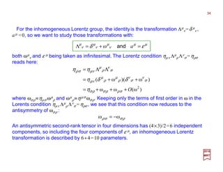
![The Relativity Principle
Einstein’s principle of relativity states the equivalence of certain ‘inertial’ frames of
reference. It is distinguished from the Galilean principle of relativity, obeyed by
Newtonian mechanics, by the transformation connecting coordinate systems in different
inertial frames.
2017
MRT
Here ηµν is the diagonal 4×4 matrix, with elements (i.e., the Minkowski metric): η00 =+1,
η11 =η22 =η33 =−1 and ηµν ≡0 for µ ≠ν. These transformations have the special property
that the speed of light c is the same in all inertial frames (e.g., a light wave traveling at
speed c satisfies |dr/dt|=c or in other words Σµνηµν dxµ dxν =c2dt2 − dr2 =0, from which it
follows that Σµνηµν dxµ dxν =0, and hence |dr /dt|=c).
If the contravariant vector xµ =(ct,r) are the coordinates in one inertial frame (x1, x2, x3)
[i.e., r = xi (i=1,2,3), as Cartesian space coordinates, and x0 =ct a time coordinate, the
speed of light being c] then in any other inertial frame, the coordinates xµ must satisfy:
OO
xdxdxdxd
FrameFrame
∑∑∑∑ = == =
≡
3
0
3
0
3
0
3
0 µ ν
νµ
µν
µ ν
νµ
µν ηη
or equivalently stated as the Principle of covariance:
∑∑ ∂
∂
∂
∂
=
µ ν
µνσ
µ
ρ
µ
σρ ηη
x
x
x
x
The covariant vector can be given as xµ=Σνηµν xν =(ct,−r). The norm of the vector
Σµ xµ xµ =(x0)−Σi(xi)2 =c2t2 −|r|2 is a Lorentz invariant term.
17](https://image.slidesharecdn.com/linked-inslides-qft-130507130813-phpapp02/85/Part-IV-Quantum-Fields-17-320.jpg)
![Poincaré Transformations
with aµ arbitraryconstants(e.g.,‘leaps’),and Λµ
ν aconstantmatrixsatisfyingthecondition:
Any coordinate transformation xµ → xµ that satisfies Σµνηµν (∂xµ /∂xρ )(∂xν /∂xσ )=ηρσ is
linear and allows us to define the Poincaré Transformations:
2017
MRT
µµµµµµ
ν
ν
ν
µµ
axxxxaxx +Λ+Λ+Λ+Λ=+Λ= ∑=
3
3
2
2
1
1
0
0
3
0
σρ
µ ν
σ
ν
ρ
µ
µν ηη =ΛΛ∑∑
The matrix ηµν has an inverse, written ηµν , which happens to have the same
components: it is also diagonal matrix, with elements: η00 =+1,η11 =η22 =η33 =−1 and
ηµν ≡0 for µ ≠ν.
To save on using summation signs (Σ), we introduce the Summation Convention:
We sum over any space-time index like µ and ν (or i, j or k in three dimensions) which
appears twice in the same term, if they appear only once ‘up’ and also only once ‘down’.
As an example, and while also enforcing this tricky summation convention, we now
multiply ηµµµµνννν Λµµµµ
ρ Λνννν
σ=ηρσ above with ησττττΛκ
ττττ and when inserting parentheses for show:
ρ
κ
ρ
κκ
ρ
κ
ρ
κ
ρ
κ
ρ ηηηηηηηηη µµµµνννν
µνµνµνµν
σσσσ
σσσσ
ττττσσσσ
ττττσσσσ
ττττσσσσ
ττττσσσσ
ννννµµµµ
µνµνµνµν
µνµνµνµν ττττσσσσ
ττττσσσσ
ττττσσσσ
ννννµµµµ
µνµνµνµν Λ=Λ=Λ=Λ=ΛΛΛ=ΛΛΛ∑ ∑ ][)(])[(])[(
44 34421
and now, when multiplying with the inverse of the matrix ηµµµµν Λµµµµ
ρ, we get from this:
ττττσσσσ
ττττσσσσ ηη κνκν
ΛΛ=
( )3,2,1,0=µ
18](https://image.slidesharecdn.com/linked-inslides-qft-130507130813-phpapp02/85/Part-IV-Quantum-Fields-18-320.jpg)
![and this unitary operator U satisfies the same group composition rule as T(Λ,a):
So, in accordance with the discussion in the previous slides, the transformations T(Λ,a)
induced a unitary linear transformation on a state vector in the Hilbert space:
For example, we will soon discuss the wave function in its momentum representation:
for which the same composition rule applies:
2017
MRT
)]()([)]([)]([),( 1
pLpLUpLUpLUpU ΛΛΛ=Λ≡Λ −
),(),(),(),;( jjj mppUmpmjp ΨΨΨΨΨΨΨΨΨΨΨΨ Λ=→µ
)(),()()( xaUxx ψψψ µ
Λ=→
),(),(),( aaUaUaU +ΛΛΛ=ΛΛ
20](https://image.slidesharecdn.com/linked-inslides-qft-130507130813-phpapp02/85/Part-IV-Quantum-Fields-20-320.jpg)
![Now it is time to study three-dimensional rotations and add relativity to the overall
description. To this effect we will exploit pretty much all the group symmetry properties!
2017
MRT
ζζβγ
ζζβγ
sinhcosh)(
sinhcosh)(
03033
22
11
30300
xxxxx
xx
xx
xxxxx
−=−=
=
=
−=−=
and v=|v| is the relative velocity of the two frames.
or (N.B., implicit sum on ν ):
β
ζ
ζ
ζβγβζ
β
ζγ ==
==
−
==
cosh
sinh
tanhsinh
1
1
cosh
2
aswellaswithand
c
v
−
−
=
3
2
1
0
3
2
1
0
cosh00sinh
0100
0010
sinh00cosh
x
x
x
x
x
x
x
x
ζζ
ζζ
that is, assuming propagation in the direction of the x3-axis. This can be represented in
matrix form as:
Let us recall a few facts about homogeneous Lorentz transformations:
where:
ν
ν
µνµµ
ζ xxxx )],-([Λ=
21](https://image.slidesharecdn.com/linked-inslides-qft-130507130813-phpapp02/85/Part-IV-Quantum-Fields-21-320.jpg)
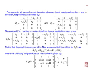
![The explicit matrix representation of a restricted homogeneous Lorentz transformation
in the x1-direction (i.e., a rotation in the x0-x1 plane) is given by:
Similarly, the infinitesimal generators M02 and M03 for rotations in the x0-x2 and x0-x3
planes respectively, are given by:
and the infinitesimal generator M10 for this rotation is defined as:
−
−
=
1000
0100
00coshsinh
00sinhcosh
)(Λ[01] ζζ
ζζ
ζ
==≡
=
0000
0000
0001
0010
)(Λ
0
[01]
10
1
ζ
ζ
ζ
d
d
MK
==≡
==≡
==
0001
0000
0000
1000
)(Λ
0000
0001
0000
0100
)(Λ
0
[03]
03
3
0
[02]
02
2
ζζ
ζ
ζ
ζ
ζ
d
d
MK
d
d
MK ,
2017
MRT
22](https://image.slidesharecdn.com/linked-inslides-qft-130507130813-phpapp02/85/Part-IV-Quantum-Fields-22-320.jpg)

![A finite rotation in the µ -ν plane (in the sense µ toν ), is again obtained by
exponentiation:
2017
MRT
ζνµ µν
ζ M
xx e),-(Λ =
µσνρνρµσµρνσνσµρρσµν
ηηηη MMMMMM −−+=],[
One verifies that the infinitesimal generators, Mµν ,satisfy the following commutation
rules:
25](https://image.slidesharecdn.com/linked-inslides-qft-130507130813-phpapp02/85/Part-IV-Quantum-Fields-25-320.jpg)
![
∂
∂
=
∂
∂
−=
∂
∂
−=
∂
∂
∂
∂
−=•
=
kj
kji
ikji
kji
k
k
k
x
xi
x
xi
x
i
x
xf
i
εε
ζ
ζ
ϕ
µ
)ˆ()ˆ()ˆ(
);(ˆˆ
0
nnrn
Jn
××××
hence:
kj
kjii
x
xiJ
∂
∂
= ε
For the rotation acting on the space-time coordinates, note that the time coordinate is
unaffected (hence only latin indices):
•−=
−•−+=
=
+−+==≡
ζζ
ζζ
ϕϕϕϕµµ
sinhˆcosh
]sinhˆ)1[(coshˆ
]ˆ[sin)]ˆ(ˆ)[cos1()],ˆ([);(
rn
nrnrr
rnrnnn
cttc
ct
xxRxfx kkki
i
k
××××××××××××
in which we made use of the relation xj =ηij xj =−x j, η being the Minkowski 3-metric. It can
be shown that the generators for rotation are equivalent to the generators for the SO(3)
Special Orthogonal group (which are Hermitian). Thus, the representation for a finite
rotation acting on the wavefunction is unitary and it is given by U(R)=exp(−iϕ n•J/h).ˆ
2017
MRT
where v=ctanhζ n. So, we get:ˆ
26](https://image.slidesharecdn.com/linked-inslides-qft-130507130813-phpapp02/85/Part-IV-Quantum-Fields-26-320.jpg)
(
ˆ j
iR
R ϕ
ν
µ
n
2017
MRT
27](https://image.slidesharecdn.com/linked-inslides-qft-130507130813-phpapp02/85/Part-IV-Quantum-Fields-27-320.jpg)
;(
x
x
x
xi
x
x
x
xi
x
x
x
x
x
x
x
xi
x
xi
x
xf
iK
ζζζζ
µ
ν
ζ
ν
µ
µ
ζ
µ
ζζζζ
ζζ
ζ
2017
MRT
28](https://image.slidesharecdn.com/linked-inslides-qft-130507130813-phpapp02/85/Part-IV-Quantum-Fields-28-320.jpg)
![Similarly:
)( 0000 iiiii xxi
x
x
x
xiK ∂−∂=
∂
∂
−
∂
∂
=
†
00
])([)()()( xKx
x
xx
x
xixK iiii ψψψψ ≠
∂
∂
−
∂
∂
=
Consider that the state-vector of the system is given by |ψ 〉, hence the action of Ki on
the state is:
This implies that the generator for the Lorentz boost, Ki, is not Hermitian and hence the
exponentiation of the generator (i.e., exp(−iζ i Ki /h)) will not be unitary. The
representation of the Lorentz boost acting on the wavefunction is not unitary and hence
is not trace-preserving.
We can summarize the effects of the rotations and the Lorentz boost into one second-
rank covariant tensor:
)( µννµµν ∂−∂= xxiM
in which Ji =½ε ijk Mjk and Ki =Mi0.
2017
MRT
29](https://image.slidesharecdn.com/linked-inslides-qft-130507130813-phpapp02/85/Part-IV-Quantum-Fields-29-320.jpg)
![These generators (i.e., Pµ and Mµν ) obey the following commutation relations, which
characterize the Lie algebra of the Poincaré group (and adding h and c for reference):
kkjijikkjijikkjiji JiKKKiKJJiJJ εεε hhh −=== ],[],[],[ and;
0],[
)(],[
)(],[
=
−−=
−+−−=
λµ
νµλµνλλµν
νρµσµρνσµσνρνσµρµνρσ
ηη
ηηηη
PP
PPiPM
MMMMiMM
h
h
The rotation Ji and boost Kj generators can be written in covariant notation Mµν and
the commutation relations are then re-written as:
2017
MRT
00
],[],[],[ P
c
iPKcPiPKPiPJ jijiiikkjiji δε
h
hh === and;
0],[0],[0],[ 00
=== jiii PPPPPJ and;
The first of these is the usual set of commutators for angular momentum, the second
says that the boost K transforms as a three-vector under rotations, and the third implies
that a series of boosts can be equivalent to a rotation. Next we have:
where P0c=H, the Hamiltonian, and finally all components of Pµ should commute with
each other:
Together, these equations above form the Lie algebra of the Poincaré group.
30](https://image.slidesharecdn.com/linked-inslides-qft-130507130813-phpapp02/85/Part-IV-Quantum-Fields-30-320.jpg)


![]ω,ω)([
]ω)(,ω)([
]ω)(,ω)([
]ω)(,ω)[(),(
])ω)((,ω)[(),(),(),ω(),(),(),ω(),(
11
111
11
ω)(ω)(
11
11
ω
111
11
11
aU
aaaU
aaU
aUaU
aUaUaUUaUaUUaU
aaaa
aaa
−−
−−−
−−
+Λ+−=Λ+=Λ=Λ=Λ
−−
−−
Λ−=Λ=Λ=+=Λ
−−−
ΛΛ−ΛΛ+Λ≡
ΛΛ+Λ+ΛΛ−Λ+Λ=
+Λ+Λ+Λ−Λ+Λ=
+Λ+−Λ+Λ=
+Λ−+Λ+Λ=Λ−Λ+Λ=Λ+Λ
−−
−−
ε
ε
ε
ε
εεε
ε
ε
1
1
11
11
1111
11
1
4444444 34444444 21
4444 34444 21
&;;
&;;
2017
MRT
where Λµ
ν and aµ are here the parameters of a new transformation, unrelated to ω and
ε.
Let us consider the Lorentz transformation properties of Pρ and Mρσ. We consider the
product:
),(),( 1
aUaU Λ+Λ −
),(1 εεεεωωωωU
In the end the transformation rule is given by:
],[),(),(),( 111
aUaUUaU −−−
ΛΛ−ΛΛΛ+≡Λ+Λ ωωωωωωωωωωωω εεεεεεεε 11
since Λ1Λ−1= 1.
According to the composition rule T(Λ,a)T(Λ,a)= T(ΛΛ,Λa+a) with T =U(Λ,a) the
product U(Λ−1,−Λ−1a) U(Λ,a) equals U(1,0), so U(Λ−1,−Λ−1a) = U−1(Λ,a), i.e., U(Λ−1,−Λ−1a)
is the inverse of U(Λ,a). It follows from U(Λ,a)U(Λ,a)= U(ΛΛ,Λa+a) that, in sufficient
detail to show these important group operations so that they be well understood, we have:
36](https://image.slidesharecdn.com/linked-inslides-qft-130507130813-phpapp02/85/Part-IV-Quantum-Fields-36-320.jpg)
![2017
MRT
Using U(1+ω,ε)=1−(i/h)ερ Pρ +½(i/h)ωρσ Mρσ to first order in ω and ε we have then:
)(ω
2
1
)(
2
1
)(
2
1
ω
ω
2
1
)(ω
2
1
])(ω[
)ω(
2
1
)ω(),(ω
2
1
),(
1
1
111
µννµµνσ
ν
ρ
µρσ
µρ
µρ
µννµνµµνσ
ν
ρ
µρσ
µρ
µρ
µνσ
ν
ρ
µρσ
µν
ν
σ
ρσ
ρ
µ
µν
ν
σ
ρσ
ρ
µ
µ
ρ
ρ
µ
µν
µν
µ
µ
σρ
σρ
ρ
ρ
ε
ε
ε
εε
PaPaM
i
P
i
PaPaPaPa
i
P
i
M
i
M
i
PaP
i
M
i
Pa
i
aUM
i
P
i
aU
−−ΛΛ+Λ−=
++−ΛΛ+
Λ−
ΛΛ+=
ΛΛ+
ΛΛ−Λ−=
ΛΛ+ΛΛ−Λ−=Λ
+−Λ
−
−
−−−
hh
h
h
h
h
h
hhhh
1
1
1
11
Equating coefficients of ωρσ and ερ on both sides of this equation we find:
)(),(),(
),(),(
1
1
µννµµνσ
ν
ρ
µ
σρ
µρ
µ
ρ
PaPaMaUMaU
PaUPaU
−−ΛΛ=ΛΛ
Λ=ΛΛ
−
−
where we have exploited the antisymmetry of ωρσ , i.e., ωρσ =−ωσρ , and we have used
the inverse (Λ−1)ν
σ =Λν
ρ =ηνµ ηρσ Λµ
ρ.
37](https://image.slidesharecdn.com/linked-inslides-qft-130507130813-phpapp02/85/Part-IV-Quantum-Fields-37-320.jpg)
![Next, let’s apply these rules rules to a transformation that is itself infinitesimal, i.e.,
Λµ
ν=δ µ
ν +ωµ
ν and aµ =ε µ, with infinitesimals ωµ
ν andεµ unrelated to the previous ω
and ε.
2017
MRT
Equating coefficients of ωρσ and ερ on both sides of these equations, we would find
these commutation rules:
µρνσρνµσσνρµµσρνρσµν
ρσµσρµρσµ
ρµ
ηηηη
ηη
MMMMMM
i
PPMP
i
PP
+−+=
−=
=
],[
],[
0],[
h
h
This is the Lie algebra of the Poincaré group.
µρ
µ
ρµ
µ
µν
µν ε PPPM
i
ω,ω
2
1
=
−
h
νρσ
ν
µσρ
µ
ρσσρµνµ
µ
µν
µν εεε MMPPMPM
i
ωω,ω
2
1
+++−=
−
h
and
By using U(1+ω,ε)=1−(i/h)ερ Pρ +½(i/h)ωρσ Mρσ and keeping only terms of first order
in ωµ
ν andε µ, our equations for Pρ and Mρσ become:
38](https://image.slidesharecdn.com/linked-inslides-qft-130507130813-phpapp02/85/Part-IV-Quantum-Fields-38-320.jpg)
![In quantum mechanics a special role is played by those operators that are conserved,
i.e., that commute with the energy operator H=P0. We just saw that [Pµ,Pρ]=0 and
(i/h)[Pµ,Mρσ ]=ηµρPσ−ηµσ Pρ shows that these are the momentum three-vectors:
2017
MRT
and the angular momentum three-vector:
These are not conserved, which is why we do not use the eigenvalues of K to label
physical states. In a three-dimensional notation, the commutation relations may be
written:
where i, j, k, &c. run over the values 1, 2, and 3, and εijk is the totally antisymmetric
quantity with ε123 =+1. The commutation relation [Ji ,Jj ]=iεijk Jk is the angular-
momentum operator.
],,[ 321
PPP=P
],,[],,[ 211332123123
JJJJJJ −−−==J
and the energy P0 itself. The remaining generators form what is called the ‘boost’ three-
vector:
],,[],,[ 030201302010
JJJJJJ −−−==K
jijikjkiji
kjkijikjkijikjkiji
iiii
HiPKPiPJ
JiKKKiKJJiJJ
PiHKHHHPHJ
δε
εεε
==
−===
====
],[],[
],[],[],[
],[0],[],[],[
and
and,
and
39](https://image.slidesharecdn.com/linked-inslides-qft-130507130813-phpapp02/85/Part-IV-Quantum-Fields-39-320.jpg)
![Now,* there is one peculiar consequence to one of these commutators – the two boost
generators are:
2017
MRT
This commutator means that two boosts, Bi and Bj , in different directions (i.e., the
indices i and j can’t equal each other at the same time) are not equivalent to a single
boost B:
where B is some boost. The reason things aren’t equal is the factor Wn××××m(Ω), the Wigner
Rotation where Ω is the Wigner Angle (i.e., a true space-time rotation although to be
realistic, for practical reason it is usually an infinitesimal one.)
BWBB )(ˆˆˆˆ Ω= mnmn ××××
kjkiji JiKK ε−=],[
)()()()( ˆˆˆˆ
1
ˆˆˆˆˆˆ Ω=ΩΩΩ= −
mnmnmnmnmn ×××××××××××××××× WBWBWWBB
* Credit for developing this in the way it is shown here (and in the next few slides), with an example of which is given pretty
much as it is, is much due to Entanglement in Relativistic Quantum Mechanics, E. Yakaboylu, arxiv:1005.0846v2, August 2010.
By using B=WBW−1, the expression Bn Bm =Wn××××m (Ω)B above can be re-written as:ˆ
ˆ ˆ
ˆ ˆ ˆ
40](https://image.slidesharecdn.com/linked-inslides-qft-130507130813-phpapp02/85/Part-IV-Quantum-Fields-40-320.jpg)

![By replacing sinΩ and cosΩ in the boost matrix Bf one gets:
2017
MRT
Notice now that this Bf matrix is symmetric. So, as a result in this case (i.e., a boost
along the x-direction followed by a boost in the y-direction), we obtain a boost along
‘some’ direction given by Ω=tan−1[− βxγx βyγ y /(γx+γy)] in the x-y plane.
+
+
+
−
++
+−
−−
=Ω= −
−
1000
0
1
)(
1
0
11
1
0
)(
ˆˆ
ˆˆˆ
ˆˆ
2
ˆˆˆˆ
ˆˆ
ˆˆ
2
ˆˆˆˆ
ˆˆ
2
ˆ
2
ˆ
2
ˆ
ˆˆˆ
ˆˆˆˆˆˆˆ
ˆˆ
1
ˆ
yx
yxy
yx
yyxx
yy
xy
yyxx
yx
yxx
yxx
yyyxxyx
xyz
γγ
γγγ
γγ
γβγβ
βγ
γγ
γβγβ
γγ
γβγ
γβγ
βγγβγγγ
BBWBf
mnmn ˆˆ
1
ˆˆ )( BBWB Ω= −
××××
Note that we can read BnBm =Wn××××m (Ω)Bf (e.g., By Bx =Wy××××x (Ω)Bf =W−z (Ω)Bf in the
example above) backward to note that any boost B in the n-m (e.g., the x-y plane in the
example above) can be decomposed into two mutually perpendicular boosts (in order)
followed by a Wigner rotation (using group algebra – we mean it’s inverse)*:
ˆ ˆ ˆ ˆ ˆ ˆ ˆ ˆ ˆ
ˆ ˆ ˆ ˆ
* Credit for this notation is based on Generic composition of boosts: An elementary derivation of the Wigner rotation, R.
Ferraro and M. Thibeault, Eur. J. Phys. 20 (1999) 143-151.
This result will be used later when we discuss particle representation in quantum field
theory using Wigner basis states and especially when we calculate one first hand…
ˆ ˆ ˆ ˆ ˆ ˆ ˆ ˆ
43](https://image.slidesharecdn.com/linked-inslides-qft-130507130813-phpapp02/85/Part-IV-Quantum-Fields-43-320.jpg)
![Since we will be using this soon let us look at a general example. Suppose that a parti-
cle of mass mo is seen from system O with momentum p along the +z-axis. A second ob-
server sees the same particle from a system O moving with velocity v along the +x-axis:
ΩΩ
Ω−Ω−Ω+Ω−−
Ω+ΩΩ−Ω
=
ΩΩ
Ω−Ω
ΩΩ
−
−
=
ΩΩ
Ω−Ω
+
+
−
−
=ΛΛ=Λ −
−−=
cos0sin
0100
sincos0cossin
sincos0cossin
cos0sin
0100
sin0cos0
cos0sin
1000
0100
00
00
cos0sin0
0100
sin0cos0
0001
00
0100
0010
00
1000
0100
00
00
),()()(
ˆˆˆˆ
ˆˆˆˆˆˆˆˆˆˆˆˆˆ
ˆˆˆˆˆˆˆˆˆˆˆˆ
ˆˆˆˆ
ˆˆˆˆˆ
ˆˆˆ
ˆˆˆ
ˆˆˆ
ˆˆˆ
ˆˆˆ
ˆˆˆ
1
ˆˆˆˆˆˆ
zzzz
xzzxxxzzxxzxx
xxzzxxxzzxzx
zzzz
zzzzz
xxx
xxx
zzz
zzz
xxx
xxx
yzxyzx
γγγβ
γγβγβγγβγβγγβ
γβγβγγβγβγγγ
γγγβ
γβγβγ
γγβ
γβγ
γγβ
γβγ
γγβ
γβγ
pWpLpL ××××
2017
MRT
+
−=Ω⇒
+
−=Ω=
Ω
Ω
Ω=Ω+−⇒Ω=Ω−Ω−
zx
zzxx
zx
zzxx
zzxxzxzxzzxx
ˆˆ
ˆˆˆˆ
ˆˆ
ˆˆˆˆ
ˆˆˆˆˆˆˆˆˆˆˆˆ
arctantan
cos
sin
cossin)(sinsincos
γγ
γβγβ
γγ
γβγβ
γβγβγγγγγβγβ
Since Lx××××z(Λp) is symmetric we can extract the [Lx××××z(Λp)]3
2=[Lx××××z(Λp)]2
3 components:ˆ ˆ ˆ ˆ ˆ ˆ
44](https://image.slidesharecdn.com/linked-inslides-qft-130507130813-phpapp02/85/Part-IV-Quantum-Fields-44-320.jpg)
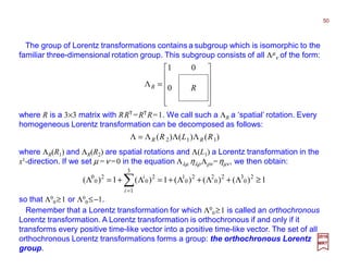
![px
W−−−−y(Λ,p)
Now, since:
This provides us with the three Cartesian values for the boosted
momentum:
2017
MRT
y
mo
Suppose that observer O sees a particle
(mass mo ≠0) with momentum pz in the z-
direction. A second observer O moves relative
to the first with velocity v in the x-direction.
How does O describe the particle’s motion?
Λp
)ˆˆ(ˆˆ ˆˆˆˆˆoˆˆ kikip zzzxxzx γβγγβ +−=+−=Λ cmpp
pz
Λ(v)
y
x
v ↑
−−
−
=
−
−
=Λ
zzz
zzxxxzxx
zzxxxzx
zzz
zzz
xxx
xxx
zx
ˆˆˆ
ˆˆˆˆˆˆˆˆ
ˆˆˆˆˆˆˆ
ˆˆˆ
ˆˆˆ
ˆˆˆ
ˆˆˆ
ˆˆ
00
0100
0
0
00
0100
0010
00
1000
0100
00
00
)(
γγβ
γβγβγγγβ
γβγγβγγ
γγβ
γβγ
γγβ
γβγ
pL
−
=
−−
−
=Λ
cm
cm
cmcm
kpL
oˆˆ
oˆˆˆ
oˆˆo
ˆˆˆ
ˆˆˆˆˆˆˆˆ
ˆˆˆˆˆˆˆ
ˆˆ
0
0
0
0
00
0100
0
0
)(
zz
zxx
zx
zzz
zzxxxzxx
zzxxxzx
zx
γβ
γγβ
γγ
γγβ
γβγβγγγβ
γβγγβγγ
µ
we then have (N.B., with kµ=[moc,0,0,0]T a standard rest momentum for massive particles):
−
=
Λ
Λ
Λ
zz
zxx
ˆˆo
ˆˆˆo
3
2
1
0
γβ
γγβ
cm
cm
p
p
p
)ˆˆ(ˆˆ ˆˆˆˆˆooˆˆoˆˆˆ kikip zzzxxzzzxx γβγγβγβγγβ +−=+−=Λ cmcmcm
x
z
z
Lz(p)
which when applied in the Figure will look like:
45](https://image.slidesharecdn.com/linked-inslides-qft-130507130813-phpapp02/85/Part-IV-Quantum-Fields-45-320.jpg)
![The Poincaré Algebra
and is a space-time translation, i.e., as the product operation of a translation by a real
vector aµ =[τ,a] and a homogeneous Lorentz transformation, Λµ
ν (the translation being
performed after the homogeneous Lorentz transformation.) It can conveniently be
represented by the following matrix equation:
The inhomogeneous Lorentz transformation (or Poincaré group), L={Λ,a}, is defined by:
2017
MRT
ΛΛΛΛ
ΛΛΛΛ
ΛΛΛΛ
ΛΛΛΛ
=
1100001
3
2
1
0
33
3
3
2
3
1
3
0
22
3
2
2
2
1
2
0
11
3
1
2
1
1
1
0
00
3
0
2
0
1
0
0
3
2
1
0
x
x
x
x
a
a
a
a
x
x
x
x
The commutation rules of these generators with themselves are the Poincaré Algebra:
µν
ν
µµµ
axx +Λ== )( xL
ρµσνρνσµµσµρµσνρρσµνρµ
ηηηη MMMMMMiPP +−−== ],[0],[ and
ρµσσµρσρµ
ηη PPMPi −=],[
where the last coordinate, i.e., 1, has no physical significance and is left invariant by the
transformation. The generators for infinitesimal translations are the Hermitian operators
Pµ, and their commutative relations with the Hermitian generators for ‘rotations’ in the
xµ -xν plane, Mµν =−Mν µ are as expressed in contravariant form:
46](https://image.slidesharecdn.com/linked-inslides-qft-130507130813-phpapp02/85/Part-IV-Quantum-Fields-46-320.jpg)
![Lorentz Transformations
We note from (detΛ)2=1 above that either detΛ=+1 or detΛ=−1; those transformations
with detΛ=+1 form a subgroup of either the homogeneous or the inhomogeneous
Lorentz group. Furthermore, from the 00-components of ηµν Λµ
ρ Λν
σ=ηρσ and Λν
σ Λκ
τ ηστ
=ηνκ, we have:
These transformations also form a group.
Now, those transformations with aµ =0 form a subgroup with to the Poincaré group:
with i summed over the values 1, 2, and 3. We see that either Λ0
0≥+1 or Λ0
0≤−1. Those
transformations with Λ0
0≥+1 form a subgroup. Note that if Λµ
ν and Λµ
ν are two such Λs,
then:
ii
ii 00
00
2
0
0
11)( ΛΛ+=ΛΛ+=Λ
0
3
3
0
0
2
2
0
0
1
1
0
0
0
0
0
0
0
0
0
)( ΛΛ+ΛΛ+ΛΛ+ΛΛ=ΛΛ≡ΛΛ µ
µ
)0,()0,()0,( ΛΛ=ΛΛ TTT
2017
MRT
Taking the determinant of ηµν Λµ
ρ Λν
σ=ηρσ gives:
so Λµ
ν has an inverse, [Λ−1]ν
σ, which we see from ηµν Λµ
ρ Λν
σ=ηρσ and takes the form:
σ
µσρ
µν
ρ
νν
ρ
ηη Λ=Λ=Λ−
][ 1
These transformations also form a group. known as the homogeneous Lorentz group.
If we first perform a Lorentz transformation Λ:
ν
ν
ρ
ρ
µρ
ρ
µµ
xxx ΛΛ=Λ=
1)det( 2
=Λ
47](https://image.slidesharecdn.com/linked-inslides-qft-130507130813-phpapp02/85/Part-IV-Quantum-Fields-47-320.jpg)

![and so:
The subgroup of Lorentz transformations with detΛ=+1 and Λ0
0≥+1 is known as the
proper orthochronous Lorentz group.
1)(1)( 2
0
02
0
0
0
3
3
0
0
2
2
0
0
1
1
0
0
0
−Λ−Λ≤ΛΛ+ΛΛ+ΛΛ≡ΛΛ i
i
But (Λ0
0)2=1+Λi
0Λi
0=1+Λ0
iΛ0
i shows that the three-vector [Λ1
0,Λ2
0,Λ3
0] has length
√[(Λ0
0)2−1], and similarly the three-vector [Λ0
1,Λ0
2,Λ0
3] has length √[(Λ0
0)2−1], so the
scalar product of these two three-vector is bounded by:
1)(1)()( 2
0
02
0
0
0
0
0
0
0
0
−Λ−Λ−ΛΛ≥ΛΛ
2017
MRT
49
If we look over the Lorentz transformation properties of Pρ and Mρσ is the case for
homogeneous Lorentz transformations (i.e., aµ =0), we get:
µνσ
ν
ρ
µ
σρ
µρ
µ
ρ
MaUMaU
PaUPaU
ΛΛ=ΛΛ
Λ=ΛΛ
−
−
),(),(
),(),(
1
1
These transformation rules simply say that Mρσ is a tensor and Pρ is a vector. For pure
translations (i.e., with Λµ
ν =δ µ
ν ), they tell us that Pρ is translation-invariant, but Mρσ is
not.](https://image.slidesharecdn.com/linked-inslides-qft-130507130813-phpapp02/85/Part-IV-Quantum-Fields-49-320.jpg)
![The problem of finding the representation of the ‘restricted’ Lorentz group is equivalent
to finding all the representations of the commutation rules above. The finite dimensional
irreducible representation of the restricted group can be labeled by two discrete indices
which can take on a values the positive integers, the positive half-integers, and zero. To
show this, let us define the operators:
2017
MRT
and their commutation rules are:
From these operators, we can construct these invariants of the group:
( )
( )
( )Boost
momentumAngular
Momentum
],,[
],,[
],,[
030201
211323
321
MMM
MMM
PPP
=
=
=
K
J
P
kijkji
kijkji
kijkji
KKJ
JKK
JJJ
ε
ε
ε
=
−=
=
],[
],[
],[
which commute with all the Ji and Ki. They are therefore the invariants of the group and
they are multiples of the identity in anyirreduciblerepresentation.The representations
can thus be labeled by the values of these operators in the given representation.
and
µν
µν MM2
122
=− KJ
ρσµν
µνρσε MM8
1=•− KJ
51](https://image.slidesharecdn.com/linked-inslides-qft-130507130813-phpapp02/85/Part-IV-Quantum-Fields-51-320.jpg)
![which satisfy the following commutation rules:
To make the range of values of the label more transparent, let us introduce the
following generators:
2017
MRT
)(
2
1
)(
2
1
iiiiii KiJiKKiJiJ −=+= and
and
It follows from the commutation rules that a finite dimensional irreducible
representation space, Vjj' can be spanned by a set of (2j +1)(2j' +1) basis vectors
| jmj, j'm'j〉 where j, mj, j' and m'j are integers or half-odd integers, −j ≤ mj ≤ j, −j' ≤ m'j ≤ j'
and in terms of which the J and K operators have the following representation:
0],[
],[
],[
=
=
=
ji
kijkji
kijkji
KJ
JiKK
JiJJ
ε
ε
jjjjj
jjjjjjjj
mjmjmmjmjJ
mjmjmjmjmjmjJiJmjmjJ
′′=′′
′′±+±=′′±=′′±
,;,,;,
,;1,)1)((,;,)(,;,
3
21
h
hm
jjjjj
jjjjjjjj
mjmjmmjmjK
mjmjmjmjmjmjKiKmjmjK
′′′=′′
±′′+′±′′′=′′±=′′±
,;,,;,
1,;,)1)((,;,)(,;,
3
21
h
hm
53](https://image.slidesharecdn.com/linked-inslides-qft-130507130813-phpapp02/85/Part-IV-Quantum-Fields-53-320.jpg)
![One-Particle States
The physical states of particles are described by the Wigner basis states |ΨΨΨΨkmo
( j,mj)〉
(which are equivalent to the states|ΨΨΨΨ(k,mj)〉) for a unitary irreducible representation
of the inhomogeneous Lorentz group (Poincaré group) with Σµ pµ p µ =p02
−p2 =(moc)2.
Thesestatesformthe Hilbert space of the theory and the momentum states |ΨΨΨΨ(p,mj)〉 can
be obtained from the standard state |ΨΨΨΨpmo
( j,mj)〉≡|ΨΨΨΨ( p,mj)〉 by a unitary transformation:
∑
+
−=′
Λ
′−•−
′Λ
Λ
=≡
j
jm
jEp
m
m
j
tE
i
j
j
j
mjpW
pE
pE
xx ),()],([e
)(
)(
)π2(
1
)()( )(
)(
2/3
ΨΨΨΨD
rp
h
h
ψψ µ
Our goal is to find eigenkets of |ΨΨΨΨpmo
( j,mj)〉 as they appear following an homogeneous
Lorentz transformation group U(ΛΛΛΛ,a) product on a state-vector |ΨΨΨΨpmo
( j,mj)〉 is as follows:
where L( p) is some standard Lorentz transformationmatrix that depends on p=pµ and the
momentum states are normalized over intermediate states andweget the coordinate ket:
),()(),( jj mkpLmp ΨΨΨΨΨΨΨΨ =
),()]([)]([)]([)]([
)(
),(
),()]([)]([
)(
),(),(),(
o
oo
1o
o
jmk
jmkjmp
mjpUpLUUpLU
pE
m
aU
mjpUU
pE
m
aUmjaU
ΨΨΨΨ
ΨΨΨΨΨΨΨΨ
LvΛ1
LvΛ1Λ
ΛΛ=
=
−
2017
MRT
The spin j corresponds to the eigenvaluesJ2= j( j +1)h2of J2 and J3 =mj h (mj = j, j −1,…,−j).
Also, U(1,a)|ΨΨΨΨkmo
( j,mj)〉 meansthesamethingas exp(−iΣµ kµ aµ)|ΨΨΨΨkmo
( j,mj)〉(pµ =hkµ ).
57](https://image.slidesharecdn.com/linked-inslides-qft-130507130813-phpapp02/85/Part-IV-Quantum-Fields-57-320.jpg)
![The Lorentz transformations associated with the Poincaré group can be constructed in
which the quantum state differs by only a mixture of the internal spin indices mj (i.e., run-
ning over the discrete values j, j −1,…,−j) but possess the same physical observables.
The effects of the inhomogeneous Lorentz transformations (e.g., acting on the Dirac
fields) can be elucidated by considering the particle states obtained from the irreducible
unitary representations of the Poincaré group. The unitary operation representing the
Lorentz transformations acting on the Poincaré generators are given by the equations
U(Λ,a)PρU−1(Λ,a)=Σµ[Λ−1]ρ
µPµ & U(Λ,a)MρσU−1(Λ,a)=Σµν [Λ−1]ρ
µ [Λ−1]σ
ν (Mµν−aµ Pν −aν Pµ).
Since the momentum four-vector commutes among each other according to [Pµ ,Pν]=0,
the particle states can be characterized by the four-momentum Pµ together with
additional internal degrees of freedom mj. The internal degrees of freedom pertain to the
spin vector which can be affected by transformations in the space-time coordinates.
and the state transforms accordingly for a space-time translation:
),(),( jj mppmpP ΨΨΨΨΨΨΨΨ µµ
=
),(e),(e),(),( j
ap
i
j
aP
i
j mpmpmpaU ΨΨΨΨΨΨΨΨΨΨΨΨ
∑∑ −−
=≡ µ µ
µ
µ µ
µ
hh1
Thus, the one-particle state is an eigenvector of the momentum operator:
2017
MRT
The components of the energy-momentumfour-vector operator Pµ all commute with each
other (i.e., [Pµ,Pν ]=0), so it is natural to express physical state-vectors in terms of
eigenvectors of the four-momentum.This four-momentum Pµ is a trusted observable!
58](https://image.slidesharecdn.com/linked-inslides-qft-130507130813-phpapp02/85/Part-IV-Quantum-Fields-58-320.jpg)
![Under space-time translations, the states |ΨΨΨΨ(p,mj)〉 transforms as:
2017
MRT
It is thus natural to identify the states of a specific particle type with the components
of a representation of the inhomogeneous Lorentz group which is irreducible.
Hence U(ΛΛΛΛ)|ΨΨΨΨ(p,mj)〉 must be a linear combination of the state vectors |ΨΨΨΨ(Λp,mj)〉:
We must now consider how these states transform under homogeneous Lorentz
transformations U(ΛΛΛΛ,0)≡U(ΛΛΛΛ) is to produce eigenvectors of the four-momentum with
eigenvalues Λp (where we use U −1 (ΛΛΛΛ,a)Pµ U(ΛΛΛΛ,a)=Σν [Λ−1]µ
ν Pν ):
),()()(),()(
),(][)(),()]()([)(),()( 11
jj
jjj
mpUpmpUp
mpPUmpUPUUmpUP
ΨΨΨΨΨΨΨΨ
ΨΨΨΨΨΨΨΨΨΨΨΨ
ΛΛ
ΛΛΛΛΛ
µ
ν
ν
ν
µ
ν
ν
ν
µµµ
Λ=Λ=
Λ==
∑
∑ −−
),(),( jj mppmpP ΨΨΨΨΨΨΨΨ µµ
=
We now introduce a label mj to denote all other degrees of freedom (i.e., all the other
total angular momentum orientations), and thus consider state-vectors |ΨΨΨΨ(p,mj)〉 with:
),(e),(),( j
ap
i
j mpmpaU ΨΨΨΨΨΨΨΨ
∑−
= µ µ
µ
h1
∑′
′
′ΛΛ=
j
j
j
m
j
m
mj mppCmpU ),()],([),()( ΨΨΨΨΨΨΨΨΛ
59](https://image.slidesharecdn.com/linked-inslides-qft-130507130813-phpapp02/85/Part-IV-Quantum-Fields-59-320.jpg)
![In other words, if a system is confronted with a homogeneous Lorentz transformation
ΛΛΛΛ, the momentum p is changed to Λp. According to Pµ |ΨΨΨΨ(p,mj)〉=pµ |ΨΨΨΨ(p,mj)〉, the one-
particle state must possess an eigenvalue of Λp as well:
in which U(ΛΛΛΛ,a)Pµ U−1(ΛΛΛΛ,a)=Σν [Λ−1]ν
µ Pν has been used for the Lorentz transformed
momentum generator. It can be seen then that U(ΛΛΛΛ)|ΨΨΨΨ(p,mj)〉 is a linear combination of
the states |ΨΨΨΨ(Λp,m′j)〉, where:
and this, believe it or not, does leave the momenta of all the particle states invariant.
∑∑ ′
′
+
−=′
′
′ΛΛ≡′ΛΛ=
j
jj
j
j
j
m
j
j
mm
j
jm
j
m
m
j
j mppmppmpU ),(),(),()],([),()( )()(
ΨΨΨΨΨΨΨΨΨΨΨΨ DDΛ
),()(),(),( 2
o jjj mpcmmpppmpPP ΨΨΨΨΨΨΨΨΨΨΨΨ == ∑∑ µ
µ
µ
µ
µ
µ
),()()(
),(])[(),()]()()[(),()0,( 1
j
jjj
mpUp
mpPUmpUPUUmpUP
ΨΨΨΨ
ΨΨΨΨΨΨΨΨΨΨΨΨ
Λ
ΛΛΛΛΛ
µ
ν
ν
ν
µµµ
Λ=
Λ== ∑−
in which Dm′jmj
( j) (Λ,p) is termed the Wigner coefficient and, as said previously, they
depend on the irreducible representations of the Poincaré group.
As a special example, the Casimir operator Σµ Pµ Pµ cannot change the value of the
momentum (i.e., its an invariant – as also stated previously):
2017
MRT
60](https://image.slidesharecdn.com/linked-inslides-qft-130507130813-phpapp02/85/Part-IV-Quantum-Fields-60-320.jpg)
![Hence, to distinguish each state, the standard four-momentum given by kµ =[moc,0,0,0] is
chosen, from which all momenta can be achieved by means of a pure Lorentz boost:
which implies that there exists a subgroup of elements consisting of some arbitrary
Wigner rotations, W, and this subgroup is called the little group.
µ
ν
ν
ν
µ
kkW =∑
Notice that a simple three-dimensional rotation, W (which is an element of the
Poincaré group), will render the standard four-momentum invariant:
It is important to distinguish that this little group is not unique in the Lorentz group but it
is actually isomorphic to other subgroups under a similarity transformation. This is
because there is no well-defined frame for the standard momentum kµ due to the
equivalence principle in special relativity.Thedefinitionofthelittle group is dependent
on the choice of the standard momentum as well as the Lorentz transformation Λ.
Wigner’s Little Group
(N.B., the standard four-momentum is non-unique and it also depends on the charac-
teristics of the particle, e.g., whether it is a massive or a massless particle).
kpLp )(=
2017
MRT
),(),(),(),(),( 2
o jjjjjj mkmmkmkmkcmmkH ΨΨΨΨΨΨΨΨΨΨΨΨΨΨΨΨΨΨΨΨ h=== J0p and&
In this momentum rest frame, the state |ΨΨΨΨ(k,mj)〉 is specified in terms of the eigen-
values of the Hamiltonian H=p0, the momentum p, and the z-component of the total
angular momentum operator J as:
61](https://image.slidesharecdn.com/linked-inslides-qft-130507130813-phpapp02/85/Part-IV-Quantum-Fields-61-320.jpg)
![When L(p) is
applied to k we
get the momentum
p. When ΛΛΛΛ is applied
next to p it becomes
Λp. When L−1(Λp) is
applied to Λp we
recover k!
So, the only functions of pµ that are left invariant by all proper orthochronous Lorentz
transformations Λµ
ν are the invariant square p2 =Σµν ηµν pµ pν, and p2 ≤ 0, also the sign of
p0. Hence, for each value of p2, and (e.g., for p2 ≤0) each sign of p0, we can choose a
‘standard’ four-momentum, kµ, and express any pµ of this class as:
where Lµ
ν is some standard Lorentz transformation that dependsonpµ,andalso implicitly
on our choice of the standard kµ. We can define the states |ΨΨΨΨ(p,mj)〉 of momentum p by:
∑=
ν
ν
ν
µµ
kpLp )(
Wigner’s little group is the Lorentz transformation
L−1(Λp) ΛΛΛΛL(p) that takes k to L(p)k =p, and then to
Λp, and then back to k, so it belongs to the
subgroup of the homogeneous Lorentz group.
Operating on this equation with an arbitrary homogeneous
Lorentz transformation U(ΛΛΛΛ), we find:
k µ =[moc,0,0,0]
pµ =Σν Lµ
ν ( p)kνΛ p=Σν Λ0
ν pν
L−1(Λ p) L(p)
ΛΛΛΛ
),()]([)(),( jj mkpUpNmp ΨΨΨΨΨΨΨΨ L=
N(p) is a numerical normalization factor to be chosen on the next slideandwhere U[L(p)]
is a unitary operator associated with the pure Lorentz ‘boost’ thattakes[moc,0] into[p0,p].
The transformation Wµ
ν (i.e., L−1(Λp) ΛΛΛΛL(p) = W(Λ, p)) thus
leaves k µ invariant: Σν Wµ
ν kν =kµ. For any Wµ
ν satisfying this
relationship, we have:
),()]()([)]([)(
),()]([)(),()(
1
1
j
jj
mkppUpUpN
mkpUpNmpU
ΨΨΨΨ
ΨΨΨΨΨΨΨΨ
LΛLL
LΛΛ
4444 34444 21
=
−
ΛΛ=
=
∑
+
−=′
′
′Λ=Λ
j
jm
j
j
mmj
j
jj
mkpmkpU ),()],([),()],([ )(
ΨΨΨΨΨΨΨΨ WW D
where the coefficients Dm′j mj
( j ) [W(Λ, p )] furnish the
representation of the little group.
2017
MRT
62](https://image.slidesharecdn.com/linked-inslides-qft-130507130813-phpapp02/85/Part-IV-Quantum-Fields-62-320.jpg)
![Normalization Factor
Using W=L−1 ΛΛΛΛL and inserting into U(ΛΛΛΛ)|ΨΨΨΨ(p,m)〉=NU[L(Λp)]U[L−1(Λp)ΛΛΛΛL(p)]|ΨΨΨΨ(p,m)〉
and using U(W)|ΨΨΨΨ(k,m)〉=Σm′ Dm′ m(W )|ΨΨΨΨ(k,m′)〉 we get:
or, recalling the definition |ΨΨΨΨ〉=NU[L(p)]|ΨΨΨΨ〉, we finally get:
2017
MRT
for which
The normalization factor N(p) is sometimes chosen to be N(p)=1 but then we would
need to keep track of the p0/k0 factor in scalar products. Instead, the convention is that:
The normalization condition is achieved using the scalar product:
∑′
′ ′ΛΛ
Λ
=
m
mm mppW
pN
pN
mpU ),()],([
)(
)(
),()( ΨΨΨΨΨΨΨΨ DΛ
∑′
′ ′ΛΛ=
m
mm mkpUpWpNmpU ),()]([)],([)(),()( ΨΨΨΨΨΨΨΨ LΛ D
0
0
)(
p
k
pN =
mmmpmp ′−′=′′ δδ )(),(),( ppΨΨΨΨΨΨΨΨ
)()(),(),(
2
kk −′=′′ ′ δδ mmpNmpmp ΨΨΨΨΨΨΨΨ
)(
)()(
)(
)(
)(
)( 0
0
0
0
pE
pE
p
p
pN
pN
p
k
pN
Λ
=
Λ
=
Λ
⇒
Λ
=Λ
and
64](https://image.slidesharecdn.com/linked-inslides-qft-130507130813-phpapp02/85/Part-IV-Quantum-Fields-64-320.jpg)

![The explicit form for W(Λ,p) is:
where the angle θ is defined by tanhθ =√[(p0)2 −mo
2c4]/p0 and the components of the
particle momentum are given by pi (i=1,2,3). The Lorentz boost L(p) transforms the
standard momentum kµ to momentum pµ. In addition, the general Lorentz transformation
ΛL for ‘pure boost’ only is written as:
( )ppkpLpLpW pL
Λ→ →ΛΛ=Λ Λ− )(1
)(),(),(
−+
= ji
ji
i
j
ppp
p
pL
ˆˆ)1(coshsinhˆ
sinhˆcosh
)(
θδθ
θθ
−+
=Λ ji
ji
i
j
L
nnn
n
ˆˆ)1(coshsinhˆ
sinhˆcosh
ξδξ
ξξ
and it can be shown that this is an element of the little group associated with the
standard vector kµ. (N.B., L(Λp) is the Lorentz boost of the momentum (Λp)µ from
standard momentum vector kµ ). Then the Wigner transformation corresponding to the
present choice of kµ is a SO(3) rotation. Furthermore, the Lorentz boost L(p) can be
computed from the boost generator Ki =Mi0=ih(xi ∂0 −x0∂i) where L(p)=exp(−icθ p•K/h).
The explicit form of L(p) is given by:
ˆ
where n is a unit vector along the direction of the boost. This transforms the
momentum pµ to a Lorentz-transformed momentum (Λp)µ.
ˆ 2017
MRT
66
One-Particle States – con’d](https://image.slidesharecdn.com/linked-inslides-qft-130507130813-phpapp02/85/Part-IV-Quantum-Fields-66-320.jpg)
![Considering now a Taylor expansion of the Wigner transformationW(Λ,p)=
L−1(Λp)ΛL(p) as well as the explicit form of the matrix for L(p) just obtained for an
arbitrary Lorentz transformation Λ:
in which the Lorentz boosts, L(p) and L(Λ,p) and the arbitrary Lorentz transformation, Λ,
are parametrized in terms of its generators. In addition, the spatial component of the
Lorentz-transformed momentum is given by pΛ=Λp (N.B., The corresponding Lorentz
boost for the Lorentz transformed momentum starting from the standard vector, kµ, is
given by tanhθ′=|pΛ|/(Λp)0, in which L(Λp)k=Λp).
K+−=Λ µν
µν
Mω
2
1
)ω( 1
thus:
KpKp •−−•′
−
≡
ΛΛ=Λ
ˆω
2
1
ˆ
1
eee
)()(),(
Λ θθ µν
µν
hh
ci
M
ci
pLpLpW
βα
β
αβα
βµν
µναα
pppM
i
pp ]ω[]ω[
2
)( +≡−≅Λ
Consider the inifinitesimal Lorentz transformation being parametrized by the anti-
symmetric tensor ωµν (expressed to first order terms of ω):
2017
MRT
Note that in the above and from now on, we restored the summation convention
where we sum over any space-time index which appears twice in the same term.
67](https://image.slidesharecdn.com/linked-inslides-qft-130507130813-phpapp02/85/Part-IV-Quantum-Fields-67-320.jpg)
![A Taylor series expansion of the Wigner transformation is considered as fallows:
thus:
In the ‘second term’ of this last equation the expression can be re-written as:
K
K
+
∂
ΛΛ∂
+=
+
∂
Λ∂
+Λ=Λ
=
−
=
=
0ω
1
0ω
0ω
ω
)]()([
ω
ω
),(
ω),(),(
µν
µν
µν
µν
pLpL
pW
pWpW
1
K
K
+
−Λ+
∂
Λ∂
+=
+
∂
Λ∂
Λ+
Λ
∂
Λ∂
+≅Λ
=
−
=
−
=
−
=
−
)(
2
)(ω)(
ω
)(
ω
)(
ω
)ω(
)(ω)()ω(
ω
)(
ω),(
0ω
1
0ω
1
0ω
1
0ω
1
pLM
i
pLpL
pL
pLpLpL
pL
pW
µν
µν
µν
µν
µν
µν
µν
µν
1
1
in which the substitution Λp=p′ has been made and, in general, L−1(p′)=ηηηηLT(p′)ηηηη.
2017
MRT
68
−+
′
′′
−
′
+
′
−
′
−
′
∂
∂
+=
∂
Λ∂
=
=
−
22
o
0
o
o
2
o
0
0ω
22
o
0
o
o
2
o
0
0ω
1
11
ω
ω)(
ω
)(
ω
p
pp
cm
p
cm
p
cm
p
cm
p
p
pp
cm
p
cm
p
cm
p
cm
p
pL
pL
kj
kj
j
k
ji
ji
j
i
δδ
µν
µν
µν
µν
1](https://image.slidesharecdn.com/linked-inslides-qft-130507130813-phpapp02/85/Part-IV-Quantum-Fields-68-320.jpg)
![Now, since (Λp)α≅pα−(i/2)[ωµν Mµν]α
β pβ≡pα+[ω]α
β pβ, we get (h=c=1):
and since ξ i =ω0i =−ωi0 and θ k =εijk ωij as well as Ji =εijk Mjk and Ki =Mi0:
βα
β
βα
βµν
µν
µν
α
µν
ppM
ip
]ω[][ω
2ω
)(
ω
0ω
≡−≅
∂
Λ∂
=
in which the axial vector is given by θθθθ=[θ 1,θ 2,θ 3]† and mi =(p××××θθθθ)i as well as:
−
•
≡
−
•
=
−
=
−
=
+−=++−=
ii
ii
k
jkjii
jj
j
k
kjii
j
k
ki
i
ji
ji
i
i
i
i
p
ppp
p
p
p
pJK
i
pMMM
i
p
mp
ξpp
θpp
ξpp
ξ
ξθεξ
ξ
θεξ
ξ
θξ βββ
β
α
0
00
0
0
0
0
0
)ˆ(
)ˆ(
)ˆ(0
]22[
2
]ωωω[
2
]ω[
××××
−−−=
∂
′∂
∑
= nm
nnmiii
i
pppp
p
][ˆˆ][
1
ω
)ˆ(
ω 00
0ω
mpmp
p
ξξµν
µν
At this junction, the sum Σmn pm[p0ξn −|p|mn] describes the relation between the
components of the momentum and its Lorentz boost.
ˆ
2017
MRT
ˆ
69](https://image.slidesharecdn.com/linked-inslides-qft-130507130813-phpapp02/85/Part-IV-Quantum-Fields-69-320.jpg)
![Assuming that any sum over the cross-terms is zero for m≠n, that is:
)ˆ(][ˆ 00
ξpmp •=−∑ ppp
nm
nnm
ξ
in which the boost vector is given by ξξξξ=[ξ 1,ξ 2,ξ 3]†. With the axial vector, θθθθ=[θ 1,θ 2,θ 3]†,
θθθθ and ξξξξ become the parameter vectors associated with the infinitesimal Lorentz
transformation Λ. In addition, the vector normal to both the axial and momentum vectors
is given by m=p××××θθθθ.
Jmpξp
p
Km
p
pξpξ
pmξp
p
m
p
ξp
m
p
ξp
ξp
p
m
p
m
p
ξp
p
•
−
−+•
−•
−−≡
−
−−+•
−
−+•
−
=
−+
•
−
−−
−+−
+−•
=
∂
Λ∂
=
−
))))××××××××
××××××××
ˆ(2)ˆ(1ˆ)ˆ(1
)ˆ(2)ˆ(1ˆ)ˆ(1
ˆ)ˆ(10
ˆˆ1ˆˆ)ˆ(]ω[ˆ]ω[ˆ1
)ˆ(
)(
ω
)(
ω
0
o
0
oo
0
o
0
0
o
0
o
0
oo
0
o
0
oo
0
o
0
o
oo
0
o
0
o
0
oo
0
oo
0
o
0ω
1
p
m
p
i
mm
p
m
p
i
p
m
p
m
p
m
p
m
p
m
p
m
p
m
p
pp
m
p
m
p
m
p
m
p
pp
mp
pppp
m
p
mm
p
mm
p
m
pL
pL
nkinniii
kkk
kj
kj
j
k
jiijjiii
jj
εξ
ξ
δξ
ξ
β
β
β
β
µν
µν
ˆ
Our equation for ωµν [∂L−1(Λp)/∂ωµν ]|ω=0L(p) above (i.e. the ‘second term’) can be
simplified by using the Lorentz boosts from the matrices for L(p) and ΛL further up, and
this can be worked out as:
2017
MRT
70](https://image.slidesharecdn.com/linked-inslides-qft-130507130813-phpapp02/85/Part-IV-Quantum-Fields-70-320.jpg)
![The third term in our Taylor expansion for W(Λ,p) above (i.e., the term obtained above
ωµν [L−1(Λp)(−½i Mµν )]|ω=0L(p)) can also be simplified in terms of its matrix elements
(Note that the expression (−½i ωµν Mµν ) can be re-written as the matrix [ω]):
Jmpθξp
p
Km
p
pξpξ
mp
p
ξm
p
ξp
m
p
ξp
m
p
ξp
m
p
ξp
•
−+−−+•
−•
−−−≡
−+−
−•
−
−
−+•
−
=
−
−
+−
−−•
−
−
−•
−
−
=
−+
−
′′
−+
′
−
′
−
′
=′−
))))××××××××
))))××××××××
ˆ(1)ˆ(
2
ˆ)ˆ(1
ˆ(1ˆ)ˆ(
ˆ)ˆ(10
)ˆˆˆˆ(ˆ)ˆ(
)(ˆ)ˆ(0
ˆˆ1
0
ˆˆ1
)](][ω)][([
o
00
oo
0
o
0
o
0
ooo
o
0
o
0
o
0
oo
0
o
o
0
oooo
o
0
o
0
oo
o
0
o
0
o
0
o
oo
0
o
0
o
oo
0
1
m
pp
i
mm
p
m
p
i
m
p
mm
p
m
mp
m
p
m
p
m
p
m
p
pmmp
m
mp
m
p
m
p
m
p
m
mp
m
p
m
p
m
mp
m
p
pp
m
p
m
p
m
p
m
p
pp
m
p
m
p
m
p
m
p
pLpL
mlimm
m
iii
kkk
lilimmlil
il
iiii
lll
lk
lk
k
l
mmkjj
k
ji
ji
i
j
εθξ
ξ
θεξξξ
ξ
δ
θεξ
ξ
δ
in which ωµν [∂( p′)α/∂ωµν]|ω=0 above has been used for the matrix reprentation of the
arbitrary infinitesimal Lorentz transformation Λ(ω).
2017
MRT
71](https://image.slidesharecdn.com/linked-inslides-qft-130507130813-phpapp02/85/Part-IV-Quantum-Fields-71-320.jpg)
![After some careful re-grouping of the terms from all the matrix elements given in ωµν
[∂L−1(Λp)/∂ωµν]|ω=0L(p) and [L−1(p′)][ω][L(p)] just obtained, the boost terms in our
expansion for W(Λ,p) has cancelled out completely and leaving behind the rotation
terms:
where Ω( p) k =−ε ijk [ωij −(piω0j −pj ω0i)/( p0 +mo)] is the Wigner angle and Jk =½ε ijk Mij
is the rotation generator for the Poincaré group.
Thus, we obtain:
J1
1
1
Jθξp
p
1
•+=
−
−
−+=
−−
−
−=
•
+
−
−≡Λ
)(
)ωω(
)(
1
ω
)(
)(
1
)(
)(
),(
00
o
0
o
0
o
0
pi
Mpp
mp
i
Mpp
mp
i
mp
ipW
ji
ijjiji
jin
njiijji
n
θεξξ
××××
−
−
−+=Λ njinnmppW εθ)ˆ(
)(
0
00
)],([ o
0
ξp
p
1 ××××
2017
MRT
72](https://image.slidesharecdn.com/linked-inslides-qft-130507130813-phpapp02/85/Part-IV-Quantum-Fields-72-320.jpg)
![The Wigner angle can be re-written as a sum of the contributions from the rotation and
the boost:
Here the angle of rotation are represented by the Euler angles θk =ε ijk ωij and the boost
parameter ξi =ξ ni =ω0i. The finite Wigner transformation is given by:
)ˆˆ(
)(
o
0
o
0
pn
p
θ
ξp
θ
××××
××××
mp
mp
p
+
−≡
+
−≡
ξ
J•
∞→
=
Λ=Λ
i
N
N
p
N
WpW
e
,
ω
lim]),ω([
ˆ
2017
MRT
73](https://image.slidesharecdn.com/linked-inslides-qft-130507130813-phpapp02/85/Part-IV-Quantum-Fields-73-320.jpg)
![The representation matrix Dmjσ
( j) [W(Λ,p)] can be constructed from the angular
momentum generators Ji explicitly, depending on the angular momentum of the particle.
For example, spin-1/2 particles will be considered to have appropriate generators as
given by J=½σσσσ according to the isomorphism between the proper Lorentz group and the
SU(2)⊗SU(2) algebra.
J•
=Λ i
pW e),(
The Wigner transformation corresponding to an arbitrary Lorentz transformation Λ is
given by:
where Ω( p)k =−½ε ijk [(piωj
0 −pj ωi
0)/(p0 +mo)] and Jk =½ε ijk Mjk in the absence of rotation.
This can also be written as:
o
0
o
0
ˆ
)(
mpmp
p
+
=
+
−≡
pnξp ××××××××
ξ
Here the boost parameters are represented by ξi =ξni =ωi
0. For an infinitesimal variation
ωµν, the transformation matrix is (e.g., spin-1/2 case described above):
ˆ
+
−
+
•+
+
−=
−
•+
−≅
•+
=Λ
×
××
3
o
0
o
0
2
o
022
32
2222
)2/1(
)(2
ˆ
!3
1
)(2
ˆ
)(2
ˆ
!2
1
1
2!3
1
22!2
1
1
2
sin
2
cos)],([
mpmp
i
mp
I
iIiIpW
p
pnpn
σ
pn
σσ
×××××××××××× ξξξ
D
2017
MRT
74](https://image.slidesharecdn.com/linked-inslides-qft-130507130813-phpapp02/85/Part-IV-Quantum-Fields-74-320.jpg)
![The representation matrix becomes (i.e., spin-1/2 case):
For the sake of convenience, I2×2 is assigned as the 2×2 identity matrix, and σσσσ as the
‘vector’ that is comprized of the Pauli 2×2 matrices [σ1,σ2,σ3]. (Note that the Wigner
angle |ΩΩΩΩ|=Ω is dependent on both the rotation and boost parameters for an arbitrary
Lorentz transformation Λ. In addition, notice that an additional normalization factor of
√[p0/(Λp)0] has been appended to the matrix so as to maintain the condition given
D†(Λ,p) D(Λ,p)=p0/(Λp)0 I2×2).
by using the well known Pauli spin vector σσσσ relation (σσσσ•a)(σσσσ•b)=(a•b)+iσσσσ•(a××××b) and
remembering that ΩΩΩΩ=ΩΩΩΩ /|ΩΩΩΩ|. Thus, with the well known sinξ=ξ−ξ 3/3!+ξ 5/5!−… and cosξ
=1−ξ 2/2!+ξ 4/4!−… identities:
•+
Λ
=Λ
2
sin)ˆ(
2
cos
)(
)],([ 0
0
)2/1(
σ1 i
p
p
pWD
+
−•+
+
−
Λ
=
+
•+
•+
Λ
=
Λ
=Λ
×
×
•
KK
K
32
220
0
2
220
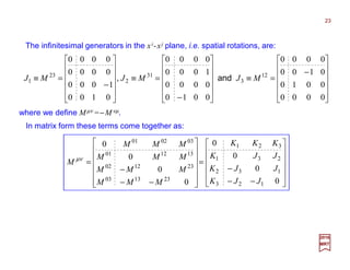
0
2
0
0
)2/1(
2!3
1
2
)ˆ(
2!2
1
1
)(
2!2
1
2!1
1
)(
e
)(
)],([
σ
σσ
σ
iI
p
p
iiI
p
p
p
p
pW
i
D
2017
MRT
ˆ
75](https://image.slidesharecdn.com/linked-inslides-qft-130507130813-phpapp02/85/Part-IV-Quantum-Fields-75-320.jpg)
]([
)]()([)],([
)2/1()2/1(1)2/1(
1)2/1()2/1(
pLpL
pLpLpW
DDD
DD
ΛΛ≡
ΛΛ=Λ
−
−
The representation matrix D(1/2)[W(Λ,p)], in the absence of rotation, is this given by:
Ω
•+
Ω
Λ
=
•−
•+
+
+Λ+
Λ
=Λ
×
××
2
sin)ˆ(
2
cos
)(
2
sinh)]ˆ([
2
sinh)ˆ(
2
cosh)(
]))[((
)/(
)],([
220
0
22o
0
22
o
0
o
0
00
)2/1(
mσ
npσnp
iI
p
p
iImpI
mpmp
pp
pW
ξξξ
××××D
)ˆˆ(sinhsinh
2
1
coshcosh
2
1
2
1
)ˆˆ(
2
sinh
2
sinh
ˆ
2
sin
)ˆˆ(sinhsinh
2
1
coshcosh
2
1
2
1
)ˆˆ(
2
sinh
2
sinh
2
cosh
2
cosh
2
cos
pn
pn
m
pn
pn
•++
=
•++
•
+
=
θξθξ
θξ
θξθξ
θξθξ
××××
&
where coshθ =p0/mo and m=n××××p represents the axis of rotation of the equivalent Wigner
transformation (e.g., of the Dirac spinors in the spin-½ case). Here the parameters ξ and
n are defined in the same manner as the general Lorentz boost as given by the ΛL
matrix.
ˆ
ˆˆ
2017
MRT
ˆ
76](https://image.slidesharecdn.com/linked-inslides-qft-130507130813-phpapp02/85/Part-IV-Quantum-Fields-76-320.jpg)
![∑−=′
′
′ΛΛ
Λ
=Λ
j
jm
j
j
mmj
j
jj
mppW
p
p
mpU ),()],([
)(
),()( )(
0
0
ΨΨΨΨΨΨΨΨ D
With the normalization and the understanding of D, our transformation thus becomes:
where Wα
µ (Λ,p)=(L−1)α
σ (Λp)⊗ Λρ
ν Lν
µ (p) is theWigner Rotation,k≡kµ =[k0 =moc,ki =0],
p≡pν =[p0 =E/c,pi ], and since U(W)|ΨΨΨΨ(k,mj)〉=Σm′j
Dm′jmj
( j) [W(Λ,p)]|ΨΨΨΨ(k,m′j)〉:
2017
MRT
since N(Λp)U[L(Λp)]|ΨΨΨΨ(k,m′j)〉=|ΨΨΨΨ(Λp,m′j)〉⇒U[L(Λp)]|ΨΨΨΨ(k,m′j)〉=N−1(Λp)|ΨΨΨΨ(Λp,m′j)〉
where the normalization constant is N(Λp)=√[k0/(Λp)0]. Finally we have:
),()],([)]([),(])()([)]([),()( 0
0
),(
1
0
0
jj
p
j mkpUpLU
p
k
mkpLpLUpLU
p
k
mpU ΨΨΨΨΨΨΨΨΨΨΨΨ ΛΛ=ΛΛ=
Λ
−
WΛΛ
W
44 344 21
444 3444 21
),(
)(
0
0
)(
0
0
),()()],([
),()],([)(),()(
j
j
jj
j
jj
mp
j
m
j
mm
j
m
j
mmj
mkpLpW
p
k
mkpWpL
p
k
mpU
′Λ
′
′
′
′
′ΛΛ=
′ΛΛ=Λ
∑
∑
ΨΨΨΨ
ΨΨΨΨ
ΨΨΨΨΨΨΨΨ
D
D
77
Isn’t this the most beautiful equation you’ve ever seen? So, this is how particle states
|ΨΨΨΨ( p,mj)〉 transform into when a Lorentz transformation Λ acts on it! That is, using a
quantum mechanical unitary operator U(Λ) that changes momentum p and spin mj!
6447481
64748p = L(p)k](https://image.slidesharecdn.com/linked-inslides-qft-130507130813-phpapp02/85/Part-IV-Quantum-Fields-77-320.jpg)
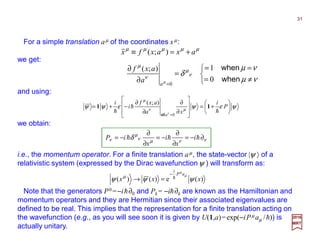
![Mass Positive-Definite
To define the mass positive-definite, we must recall a few definitions such as the unitary
quantum transformation for coordinate and angular momenta:
where P={P1,P2,P3}, J={M23,M31,M12} and K={M10,M20,M30} and their properties are
P
ρ†
=P
ρ
, M
ρσ †
=M
ρσ
and M
ρσ
=−M
σρ
. Now for the definition of invariance under a unitary
transformation of a homogeneous Lorentz Transformation Λ and a uniform translation a:
...ω
2
1
),ω( ++−=+ ρσ
ρσ
ρ
ρεε M
i
PU
h
11
),(),(),(),ω1(),( 1
jj mpmpaUUaU ΨΨΨΨΨΨΨΨ =Λ+Λ −
ε
which also applies to both momenta:
)(),(),(),(),( 11 µννµµνσ
ν
ρ
µ
µνµρ
µ
µ
PaPaMaUMaUPaUPaU +−ΛΛ=ΛΛΛ=ΛΛ −−
&
For the momentum, they commute with each other:
0],[ =νµ
PP
but for the angular momentum they do not:
ρµσσµρρσµ
ηη PPMPi −=],[
nor do the angular momenta together commute:
ρµσνρνσµνσµρµσνρρσµν
ηηηη MMMMMMi +−−=],[
As comparison, we show the case when Λ=1 then a= 0 and a rotation around the 3-axis:
θµ
µ
pJ ˆ
3 e)0,(e),1(
•−−
== hh
i
aP
i
RUaU and
( ))()0,( Λ=Λ UU
2017
MRT
78](https://image.slidesharecdn.com/linked-inslides-qft-130507130813-phpapp02/85/Part-IV-Quantum-Fields-78-320.jpg)
(
Ω•−•−
′ ′=′=Ω
pJJ
hhD
∑∑ ′
′
′
′Ω=′Ω′=Ω
j
jj
j m
j
j
mm
m
jjjj mRmmjRmjmjR )]([,)]([,,)]([ )(
DDD
θϕ
θϕ j
jjjj
j
jj
mi
kmmkmmj
mi
k jjjj
jjjjkj
mm
kmmkmjkmjk
mjmjmjmj
e
2
sin
2
cose
)!()!()!(!
)!()!()!()!(
)1(),,(
222
)(
+−′−′−+
′
Ω
Ω
+−′−′−−+
′−′+−+
−=Ω ∑D
∑∑∑ Ω=′⇒Ω= ′
l
ll
l
l
l
l
l
ll llll
m
mm
m
mmmmR zpzp ˆ,),,(ˆ,ˆ,,)]([ˆ )(
ϕθDD
2017
MRT
Recall also that your mathematical toolbox consists of these fundamental relations:
and
with
Finally:
jjjjjj
mm
j
kikimm
j
mm M
i
′′′ Ω+=Ω+ ][
2
)( )()(
δ1D
In this instance, we take (i.e., Weinberg’s QFT definition – he also uses Θ for our Ω):
where Rik =δik +Ωik with Ωik =−Ωki infinitesimal and for mj running over j, j−1,…, −j. Also:
jjjjjj
jjjjjj
mmjmm
j
mm
j
z
mmjjmm
jj
mm
jj
mJMJ
mjmjJiJMiMJ
′′′
±′′′±
==⇒
+±=±=±⇒
δ
δ
h
hm
)()(
)1)(()()(
)(
3
)(
12
1
)(
2
)(
1
)(
31
)(
23
79](https://image.slidesharecdn.com/linked-inslides-qft-130507130813-phpapp02/85/Part-IV-Quantum-Fields-79-320.jpg)
![Now, let us expand |ΨΨΨΨ(Λp; j,mj)〉=|ΨΨΨΨ(Λp)〉|l,s; j,mj 〉 in the case of an electron (s=±½):
2017
MRT
∑ +−−++−−−−+−−+
−+−+−+−
×
+++
+−+−+−+
+=≡
k ss
jjss
k
sjjs
j
mm
kmsjkmjkmskmkjsk
mjmjmsmsmm
sj
jsjsjjs
mmmmjsmmss
)!()!()!()!()!(!
)!()!()!()!()!()!()1(
)!1(
)12()!()!()!(
),(,;,,;,
ll
ll
ll
lll
ll
l
lll
lll
δC
Using Jz|l,s;j,mj 〉=mjh|l,s;j,mj 〉 we found out that that |l,s;j,mj 〉 is an eigenfunction of Jz
and since Jz commutes with J2 the eigenfunction of Jz is simultaneously an eigenfunction
of J2 which means that |l,s;ml,ms 〉 is not an eigenfunction of J2. To get around this, we
constructed a linear combination of |l,s;ml,ms 〉 instead:
such that |l,s; j,mj 〉 is simultaneously an eigenfunction of Jz and J2. The quantities Cj
mlms
=
〈l,s;ml,ms |l,s; j,mj 〉 are numerical coefficients which are known as Clebsch-Gordan (CG)
coefficients – and for our benefit j=l+s and mj =ml +ms. A general formula for these
coefficients is due to Wigner:
with l=0,1,2,…, s=±½, j =0,1/2,1,3/2,…, ml =l,l−1,…,−l, ms =±s & mj = j, j −1,…,−j.
∑ ∑′
′ Λ′Λ
Λ
=ΛΛ
j s
sj
m mm
sj
j
mmmsj pmmsmjspWmms
p
p
mjpU
l
l ll lll )(,;,,;,)],([,;,
)(
),;()( )(
)(0
0
ΨΨΨΨΨΨΨΨ D
∑∑
±=
+=
±=
==
)½(
½
,;,,;,,;,,;,,;,
s
mmm
s
j
mm
mm
jssj
sj
s
s
mmsmjsmmsmmsmjs
l
l
l
l
l
ll lllll C
80](https://image.slidesharecdn.com/linked-inslides-qft-130507130813-phpapp02/85/Part-IV-Quantum-Fields-80-320.jpg)
![a•+
∂
∂
=
∂
∂
+
∂
∂
+
∂
∂
+
∂
∂
=∇ ∇∇∇∇
t
a
z
a
y
a
x
a
t
a
a tzyxt
µµ
Point P at the tip of the distance vector xµ ={ct,r} is given in 4-dimensional Rectangular
(Cartesian) Coordinates by the intersection of constant x, constant y and constant z
planes and time t. The speed of light c is a constant of motion (the same everywhere!)
∂
∂
=
∂
∂
−
∂
∂
−
∂
∂
−
∂
∂
=∇ φ
φφφφφ
φµ ∇∇∇∇,,,,
tzyxt
x
r
O
The Laplacian ∇∇∇∇• ∇∇∇∇≡∇2 =∂2/∂x2+∂2/∂y2 +∂2/∂z2
leads to the D’Alembertian:
The divergence ∇∇∇∇• A=∂Ax /∂x+∂Ay/∂y +∂Az/∂z gives:
P
2017
MRT
A
],[],,,[ atzyxt aaaaaa ==µ
y
φ
z
If the scalar product is A•B =Ax Bx +Ay By +Az Bz, then:
ba•−=−−−= ttzzyyxxtt babababababa µµ
−
∂
∂
=
∂
∂
−
∂
∂
−
∂
∂
−
∂
∂
∇ ∇∇∇∇,,,,
tzyxt
µ
The gradient ∇∇∇∇ψ =∂ψ/∂xi +∂ψ/∂yj+ ∂ψ/∂zk of a
scalar function ψ :
ˆ ˆ ˆ
Del ∇∇∇∇=∂/∂xi+∂/∂yj+∂/∂zk =[∂/∂x,∂/∂y,∂/∂z] is now:ˆ ˆ ˆ
τ = ct
Boosts & Rotations
Electrodynamics provides the differential equations for the
potentials: φ =ρ /εo and A= j/εo and the continuity
equation: ∂φ/∂t + ∇∇∇∇•A=0. In this new in four-dimensional
notation: Aµ ={φ,A} we get Aµ = jµ/εo and ∇µ Aµ =0.
y
z
x
y
z
x
x0 = ct v
The transformation laws which give φ and A in a moving
system in terms of φ and A in a stationary system. Since
Aµ ={φ,A} is a four-vector, the equation must just look like
t= γ(t −|v|z/c2) and z= γ(z −|v|t) with γ =(1 −|v|2/c2)−1/2 except
that t is replaced by φ, and r is replaced by A. Thus:
v
22
2
)(1)(1 c
A
AAAAA
c
cA z
zxxyy
z
v
v
v
v
−
−
===
−
−
=
φφ
φ ,,,
If the vector A = Axi + Ay j+ Azk =[ Ax , Ay , Az ], then
we have the definition of the 4-vector aµ :
ˆ ˆ ˆ
=∇−
∂
∂
=
∂
∂
−
∂
∂
−
∂
∂
−
∂
∂
=∇∇ 2
2
2
2
2
2
2
2
2
2
2
tzyxt
µµ
So = (1/c2)∂t−∇2 =ηµν ∂µ∂ν =∂µ∂µ with ∂µ =∂/∂µ.
81](https://image.slidesharecdn.com/linked-inslides-qft-130507130813-phpapp02/85/Part-IV-Quantum-Fields-81-320.jpg)
![ρσ
ρσ
ρ
ρ M
i
P
i
UaU ω
2
1
ε)εω,(),(
hh
+−=+=Λ 11
]ωinTerms[)ωω()ωδ)(ωδ( 2
O+++=++=ΛΛ= ρσσρσρσ
ν
σ
ν
ρ
µ
ρ
µ
µνσ
ν
ρ
µ
µνρσ ηηηη
µµ
ν
µ
ν
µ
ν
µ
εω =+=Λ aδ and
−
−
=
−+−
−
=Λ==
)(
)(
ˆˆ)1(100
0100
0010
00
2
ctz
y
x
zt
z
y
x
t
c
c
xx
z
y
x
t
v
v
vvv
v
γ
γ
γγ
γγ
νµ
ν
µ
The Lorentz transformation transformsframe xν (say x,y,z,t) intoframe x µ (say x, y,z,t):
assuming the inertial frameis going in the x3 (+z) direction.If both ω µ
ν and εµ are taken to
be an infinitesimal Lorentz transformation and an infinitesimal translation, respectively:
This allows us to study the transformation:
The linear unitary operator U=1+iε T was constructed:
where the generators G of translation (Pµ ) and rotation (Mµν ) are given by P1, P2, and
P3 (the components of the momentum operator), M23, M31, and M12 (the components of
the angular momentum vector), and P0 is the energy operator.
2017
MRT
x2 = y
x3 = z
x1 = x
x2 = y
x3 = z
x1 = x
x0 = ct β =|v|/c
82](https://image.slidesharecdn.com/linked-inslides-qft-130507130813-phpapp02/85/Part-IV-Quantum-Fields-82-320.jpg)
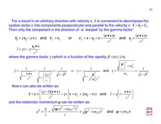
![These equations can be expressed in matrix form as:
ν
ν
µ
ν
µµ
γ
γ
γ
γ
x
x
x
x
ctx
ct
c
c
tc
x
x
x
tcx
x Λ=
=
Λ=
−+−
−
=
=
=
=
3
2
1
0
3
2
1
0
ˆˆ)1( rvv1
v
v
r
T
T
where 1 is the identity matrix, v is velocity written as a column vector, vT is its transpose
(i.e., the equivalent of a row vector) and v is its unit vector.
−+−−−
−−+−−
−−−+−
−−−
=
−+−
−
=Λ
2
2
ˆ
2
ˆˆ
2
ˆˆ
ˆ
2
ˆˆ
2
2
ˆ
2
ˆˆ
ˆ
2
ˆˆ
2
ˆˆ
2
2
ˆ
ˆ
ˆˆˆ
)1(1)1()1(
)1()1(1)1(
)1()1()1(1
ˆˆ)1(
)(
β
β
γ
β
ββ
γ
β
ββ
γγβ
β
ββ
γ
β
β
γ
β
ββ
γγβ
β
ββ
γ
β
ββ
γ
β
β
γγβ
γβγβγβγ
γ
γ
γ
γ
ν
µ
zyzxz
z
zyyxy
y
zxyxx
x
zyx
vv1
v
v
v
T
T
c
c
More generally for a boost in any arbitrary direction [β x =vx/c,β y =vy/c,β z =vz/c]:
2017
MRT
ˆ ˆ ˆ ˆ ˆ ˆ
ˆ
84](https://image.slidesharecdn.com/linked-inslides-qft-130507130813-phpapp02/85/Part-IV-Quantum-Fields-84-320.jpg)
![
−+−−−
−−+−−
−−−+−
−−−
=
−+−
−
=
2
32313
2
3
32
2
212
2
2
3121
2
1
2
1
2
3
2
2
2
1
2
2
ˆ)1(1ˆˆ)1(ˆˆ)1(1ˆ
ˆˆ)1(ˆ)1(1ˆˆ)1(1ˆ
ˆˆ)1(ˆˆ)1(ˆ)1(11ˆ
1ˆ1ˆ1ˆ
ˆˆ)1(ˆ1
ˆ1
)(
pppppp
pppppp
pppppp
ppp
ppp
p
γγγγ
γγγγ
γγγγ
γγγγ
γδγ
γγ
µ
ν
T
T
jijii
i
pL
Now, since we are using a momentum p represention we generally have for a boost in
any arbitrary direction kµ =[k0 =moc,ki =0] with pν =[p0 =E/c,pi ]:
2017
MRT
where 1 is the unit/identity matrix, p is the momentum written as a column vector, pT is its
transpose (another row vector) and p is the momentum direction unit vector and since γ
=1/√(1−β 2)=1/√(1−|v|2/c2), we have γβ =√(γ 2−1) and p=γ mov with |p|=γ mo|v|. With
these, we also have a unit vector p parallel to the direction of v:
ˆ
ˆ ˆ
o
42
o
22
ˆˆ
m
cmci
iii
+
≡≡⇒=
p
p
p
pppp γand
The result is:
=
=
=
===
=
333
33
322
33
311
330
0
3
o
3
323
22
222
22
211
220
0
2
o
2
313
11
212
11
111
110
0
1
o
1
3
3
0
o
02
2
0
o
01
1
0
o
00
0
0
o
0
ˆˆ)(ˆˆ)(ˆˆ)(0)(
ˆˆ)(ˆˆ)(ˆˆ)(0)(
ˆˆ)(ˆˆ)(ˆˆ)(0)(
0)(0)(0)()(
)(
pppppp
pppppp
pppppp
pLppLppLpppLmp
pLppLppLpppLmp
pLppLppLpppLmp
ppLmpppLmpppLmpppLmp
pL µ
ν
85](https://image.slidesharecdn.com/linked-inslides-qft-130507130813-phpapp02/85/Part-IV-Quantum-Fields-85-320.jpg)
![2017
MRT
Since the maximum momentum can be moc and the unit time vector labelled êt (which
allows us to set the standard momentum as p0 =E/c):
⊗
⊗=
=
z
y
x
t=cvp
k
k
e
e
e
eo
ˆ
ˆ
ˆ
][
]ˆ[][
zyx kkk
cm
µ
=
=
=>
κ
κ
µµ
0
0
0
0
0
0
0
0 oo mm
k
k
k and
and ki ⊗êj is the input standard momentum direction p=hk. This gives us the column
kets:
ˆ ˆ
86](https://image.slidesharecdn.com/linked-inslides-qft-130507130813-phpapp02/85/Part-IV-Quantum-Fields-86-320.jpg)
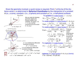
![J
To calculate this rotation, we need to choose a standard boost L(p) which carries the
four-momentum from kµ = [moc,0,0,0] to pµ. From above, this is conveniently chosen as:
jijijijij
i
i
i
ii
i
pL
cm
pLpL
cm
p
pL
pppp
p
p
p
ˆˆ)1()1(coshˆˆ)(
ˆ1sinhˆ)()(
cosh)(
2
o
0
0
o
0
0
0
−+=−+=
−====
===
γδθδ
γθ
γθ
where θ =p/moc. Here pi is the same unit vector pi/|p|, and γ =√(|p||||2 +mo
2c2)/moc=p0/moc.ˆ
2017
MRT
hh
hh
jzjjjz
jj
mJmjmmjJ
jjmjjjmj
=⇒=
+⋅=⇒+⋅=
,,
)1(,)1(, 22
JJ
| ΨΨΨΨO ( p,mj )〉
mo
Jz = mj h
p
Suppose that observer O sees a particle
(spin-mj and mass mo ≠0) with momentum p in
the y-direction and spin z-component mj . A
second observer O moves relative to the first
with velocity v in the z-direction. How does O
describe the relativistic particle’s state?
Note that for a massive particle (i.e., of mass mo and four-mo-
mentum pµ =[p0c,p]) the standard boost L(p) may be written as:
−+
−
−
−
−+
−
−
−
−+
=
2
2
3
2
o
0
2
23
2
o
0
2
13
2
o
0
o
3
2
32
2
o
0
2
2
2
2
o
0
2
12
2
o
0
o
2
2
31
2
o
0
2
21
2
o
0
2
2
1
2
o
0
o
1
o
3
o
2
o
1
2
o
0
1111
1111
1111
)(
p
p
cm
p
p
pp
cm
p
p
pp
cm
p
cm
p
p
pp
cm
p
p
p
cm
p
p
pp
cm
p
cm
p
p
pp
cm
p
p
pp
cm
p
p
p
cm
p
cm
p
cm
p
cm
p
cm
p
cm
p
pL
88](https://image.slidesharecdn.com/linked-inslides-qft-130507130813-phpapp02/85/Part-IV-Quantum-Fields-88-320.jpg)
![J
]cos,sinsin,cossin[ˆ θϕθϕθ=p
where 0≤θ ≤π and 0≤ϕ ≤2π.
θϕ
θϕ
23
ee)]ˆ([
)()(0
01
)ˆ()ˆ()ˆ(
23
1
J
i
J
i
RU
RR
RRR hh=⇒
==−
pppp RR
Now, suppose we take p to have polar (θ ) and azimutal (ϕ) angles:ˆ
2017
MRT
In this case, for a particle of mass mo =0 and helicity-σ, we have:
with the little-group element W(Λ,p) (the Wigner rotation) given by:
)ˆ()()ˆ()ˆ()ˆ()ˆ()()(),( 1111
ppBpppBpW −−−−
== RRRRpRpRp RRRRRRRR RRRR
Then we can take R(p) as a rotation by angle θ around the 2-axis, which takes [0,0,1]T
into [sinθ ,0,cosθ]T, followed by a rotation by the angle ϕ around the 3-axis:
ˆ
Suppose that observer O sees a massless
particle (helicity-σ and mass mo = 0) with unit
momentum p in the z-direction with basis ket |k〉
=col[0,0,1]. R2(p) rotates |p〉 by angle θ around
the y-axis into col[sinθ ,0, cosθ ]. Then R3(p)
rotates |p〉 by the angle ϕ around the z-axis.
ˆ
1
0
0
)( pB1.
col[sinθ , 0,cosθ ]
y
x
zϕ
First
Rotation
θ
Second
Rotation
|p〉ˆ
1
0
0
)()(2 pBR θ2.
3.
=
1
0
0
)()()()( 23 pBRRpRB θϕ
| k 〉 = col[0,0,1]
U[R(p)]|ΨΨΨΨ(p,mj)〉
U[L(Rp)R(p)B(|p|)]|ΨΨΨΨ(k,mj)〉ˆ
|ΨΨΨΨ( p,mj)〉 = |p〉×|mj 〉ˆ
ˆ
pˆ
∑
∑
∑
′
−−−
′
+
−=′
′
+
−=′
−
′
′=
′=
′=
=
−
j
jj
j
jj
j
jj
m
j
j
mm
j
jm
j
j
mmj
j
jm
j
j
mm
jj
mkRBRRBRB
p
B
mBB
p
B
mpBU
mpB
p
B
mpUB
p
B
mpBU
),(])ˆ()()ˆ()ˆ()()ˆ([)(
)(
),()],([)(
)(
),()(
),(])()([)(
)(
),()()(
)(
),()(
)ˆ(
1
)ˆ(
11)(
0
0
)(
0
0
1)(
0
0
0
0
1
ΨΨΨΨ
ΨΨΨΨΨΨΨΨ
ΨΨΨΨ
ΨΨΨΨΨΨΨΨ
444 8444 764444 84444 76 pLpL
ppppppp
p
ppWp
p
pLpLp
p
p
p
RRRR
RRRR
RRRR
R
RRD
D
RD
R
∑
+
−=′
′′=
j
jm
jjjj
j
mpmjRmjB
p
B
mpBU ),(,)]([,)(
)(
),()( 0
0
ΨΨΨΨΨΨΨΨ θp
p
since Rp = R(p)p and B(|p|) is a Lorentz boost. We finally get:ˆ
ˆ ˆ
ˆ
ˆ
σE/c
≈≈≈≈
89](https://image.slidesharecdn.com/linked-inslides-qft-130507130813-phpapp02/85/Part-IV-Quantum-Fields-89-320.jpg)
![2017
MRT
−
−
=
γγ
γγ
001
0100
0010
100
)(
2
2
pB
As just shown, it is very important to note that when Λµ
ν is an arbitrary three-
dimensional rotation R(3), the Wigner rotation W(Λ,p) is the same as R(3) for all p. To
see this, note that the boost Lµ
ν (p) above may be expressed as L(p)=R(p)B(|p|)R−1(p),
where R(p) is a rotation that takes the 3-axis into the direction of p, and:
ˆ ˆ
ˆ
)ˆ(
001
0100
0010
100
)ˆ(
1000
0cossin0
0sincos0
0001
)ˆ(
001
0100
0010
100
)ˆ(
)]ˆ()()ˆ([)]ˆ()()ˆ([
)()(),(
1
2
2
1
2
2
1
111
1
pppp
ppBpppBp
LLW
−
−
−
−−−
−
−
−
ΩΩ−
ΩΩ
−
−
=
=
=
RRRR
RRRR
ppp
γγ
γγ
γγ
γγ
RR
RRR
RR RRRR
Then, for a three-dimensional rotation RRRR, we have the following Wigner rotation about
the 3-axis with L(p)=R(p)B(|p|)R−1(p) and L(Bp)=R(Rp)B−1(|p|)R−1(Rp):ˆ ˆ ˆ ˆ
90](https://image.slidesharecdn.com/linked-inslides-qft-130507130813-phpapp02/85/Part-IV-Quantum-Fields-90-320.jpg)
![2017
MRT
The state of a moving massive particle can be shown to have exactly the same trans-
formation under rotation as in non-relativistic quantum mechanics (i.e., W(Λ= R,p)= R).
)(
100
0cossin
0sincos
100
0cossin
0sincos
cos0sin
010
sin0cos
100
0cossin
0sincos
)ˆ()ˆ( 3
1
ϕϕϕ
ϕϕ
αα
αα
ββ
ββ
γγ
γγ
RRR =
−=
−
−
−=−
pp RR
ϕ
ϕ
3
e)]ˆ([
)(0
01
)ˆ()ˆ()ˆ(
3
1
J
i
RU
R
RRR h=⇒
==−
pppp RR
Even in this general case, the rotation R−1( Rp) R R(p) takes the 3-axis into the
direction p, and then into the direction Rp, and then back to the 3-axis, so it must
be just a rotation by some azimutal angle ϕ around the 3-axis:
ˆ
ˆˆ
ˆ
444 8444 764444 84444 76 )(
1
)ˆ(
11
)ˆ()()ˆ()ˆ()()ˆ(),(
1
p
RBRRBRp
LpL
ppppppW −−−
−
= RRRR
R
and:
In conclusion, the Wigner’s formula (J3 ∝ϕ)for the d-matrixelementsd m′jmj
( j) (ϕ) still form
a Unitary Group U(ϕ) and most of all, the whole of the dictionary we have learnt already
for the Spherical Harmonics, the Clebsch-Gordan coefficients and the Wigner-Eckart
Theorem apply in the same exact way in relativistic field theory as it does in quantum
mechanics – as it does for any problem in which Dm′jmj
( j) [W(Λ,p)] for all spin-j!
Then, for an arbitrary rotation R we see that R−1( Rp) RR(p) since it is given by:ˆˆ
91](https://image.slidesharecdn.com/linked-inslides-qft-130507130813-phpapp02/85/Part-IV-Quantum-Fields-91-320.jpg)
![]0,,0,[]0,ˆ,0[ˆ 22
0
ppp cEpcEp =⇒== µ
and
ppp Λ=
Λ⇒Λ=Λ⇒=
0
0
0
)(])([)()( LkLpkpLp µµµ
µ
νν
Now, for the W-boson problem (see Figure). This first problem requires us to take p as:ˆ
2017
MRT
For a particle of rest mass MW >0 and spin σ =1 we have the
one-particle state which is mass positive-definite for the W-boson:
with the Wigner Rotation W(Λ, p), which is given by the following
group multiplication:
])1,()(
)0,()(
)1,()([
)(
),()(
)(
)1,()](
)1(
11
)1(
10
)1(
110
0
1,0,1
)1(
10
0
+ΛΩ+
ΛΩ+
−ΛΩ
Λ
=
′ΛΩ
Λ
=+=Λ
++
+
+−
+−=′
+′∑
p
p
p
p
p
p
p
p
pU
ΨΨΨΨ
ΨΨΨΨ
ΨΨΨΨ
ΨΨΨΨΨΨΨΨ
D
D
D
D
σ
σ σσ
0
0
0
)(
WcM
pL
y
z
Ω
p2
| k 〉 = [MW c,0,0,0]T
ΛΛΛΛL(p)ˆ
We can take |k〉=[0,0,0]T into p2 using L(p) as a boost along p2 followed by a boost Λ(β3)
with rapidity β3 along the 3-axis, which takes [0,p2,0]T into something like [0, p2,−p3]T:
ˆ ˆ
)()(),( 1
ppp LΛLW Λ=Λ −
with E=√[( p2c)2 +(MWc2)2]. and the unit momentum is, by definition for massive particles:
Quantum Fields – Problem 1.
]0,0,0,[ WcMk =µ
Suppose that observer O sees a W boson
(spin-1 and mass MW ≠0) with momentum p2 in
the y-direction and spin z-component Jz = σh =
h. A second observer O moves relative to the
first with velocity v in the z-direction. How does
O describe the |ΨΨΨΨ(p,σ)〉 state?
= [0,p2 , − p3 ]T| Λp 〉 ˆ ˆ MW
ˆ
ˆ
ˆ
ˆ ˆ
92
22
W
2
2 )()( cMcpE +=](https://image.slidesharecdn.com/linked-inslides-qft-130507130813-phpapp02/85/Part-IV-Quantum-Fields-92-320.jpg)

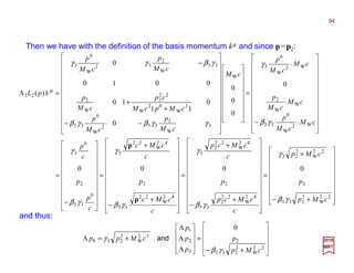
![k
v
v
jkjkjip ˆ
)(1
ˆˆ
1
ˆˆˆˆ0
2
22
W
2
2
2
2
3
22
W
2
23
2
22
W
2
2332
c
cMpc
p
cMp
pcMpp
−
+
=
−
+
=+=Λ −−−−−−−−−−−−++++
β
β
γβ
Finally we get the eigenvector for the boosted momentum Λp:
k
v
v
jk
v
v
jkjpp ˆ
1
1
ˆˆ
1
ˆˆˆ
2
W
2
W
2
2
2
22
W
2
2
232
−
+
=
−
+
==Λ≡Λ
c
cM
cM
p
c
p
c
cMp
c
ppp −−−−−−−−−−−−
so that:
x
Λ3(v)
L2(p)
W−1(Ω)
2017
MRT
y
z
| k 〉col[MW c,0,0,0] =
We see that the effect of a Lorentz boost L2(p) on the initial unit
momentum p2 followed by a Lorentz transformation Λ3(v) which
has the effect of creating (as seen from O) a momentum vector p3
in the negative 3-axis direction:
Jz =h
Suppose that observer O sees a W boson
(spin-1 and mass MW ≠0) with momentum p2 in
the y-direction and spin z-component Jz = σh =
h. A second observer O moves relative to the
first with velocity v in the z-direction. How does
O describe the |ΨΨΨΨ(p,σ)〉 state?
p2
p3
2
W
2
W
2
3
1
1
−
+
−=
c
cM
cM
p
c
p
v
v
The effect of the Wigner rotation W(Λ,p) will produce a rotation
(negative in this case) around the 1-axis which results in an angle
Ω between the 2-axis and the boost vector Λp ≡p2 j −−−− p3k.*
J
MW
ˆ
ˆ
ˆ ˆ
*It is sad to say but in many texts authors suggest that to find the answer to this problem you
only have to calculate the Wigner rotation W(Λ, p)=L−1(Λp)ΛL(p), then extract the angle Ω
and calculate D ( j)
m′jmj
=exp(iΩ J/h). The derivation that follows will be a little more practical.
ˆ
95](https://image.slidesharecdn.com/linked-inslides-qft-130507130813-phpapp02/85/Part-IV-Quantum-Fields-95-320.jpg)
![2017
MRT
Using group properties described earlier, with the vector product of the 3- and 2-axis:
)()(),( 23
1
23123 pLpLpW ΛΛ=Λ −
−= ××××××××
ΩΩ
Ω
+
+−Ω
+
+
ΩΩ
−
−
=
ΩΩ
Ω−Ω
+
+
−
−
=ΛΛ=Λ −
−
cossin00
sin
)(W
1cos
)(
10
0010
sincos0
00
0100
0010
00
cossin00
sincos00
0010
0001
1000
0
)(
10
0010
00
00
0100
0010
00
),()()(
2
W
02
22
2
2
W
02
W
22
2
W
2
W
2
W
2
2
W
0
333
333
2
W
02
W
22
2
W
2
W
2
2
W
0
333
333
1
12323
cMpcM
cp
cMpcM
cp
cM
p
cM
p
cM
p
cM
p
cMpcM
cp
cM
p
cM
p
cM
p
pWpLpL
γγβ
γβγ
γγβ
γβγ
××××
and since L(Λp)L−1(Λp)=1 we can then go through the matrix multiplicationwiththe order:
)()()()()( 1
123
1
23
1
1123 ΩΛΛ=ΩΩ −
−
−−
−−= WpLpLWW ××××××××
444 3444 21
1
we get:
)()()]()([)( 1
123
1
232323 ΩΛΛΛ=⋅Λ −
−
−
WpLpLpLpL ×××××××××××× 1
then:
96](https://image.slidesharecdn.com/linked-inslides-qft-130507130813-phpapp02/85/Part-IV-Quantum-Fields-96-320.jpg)
![2017
MRT
We finally obtain for the boost matrix L3××××2 (Λp) as a function of the deflection angle Ω:
Ω+Ω−Ω+Ω−
Ω
+
+−Ω
+
+
Ω−ΩΩ+Ω
=Λ
cossinsincos0
sin
)(
1cos
)(
10
0010
cossinsincos0
)(
3
W
2
333
W
2
332
W
0
33
2
W
02
W
22
2
2
W
02
W
22
2
W
2
33
W
2
33
W
2
32
W
0
3
23
γγβγγβγβ
γβγβγγ
cM
p
cM
p
cM
p
cMpcM
cp
cMpcM
cp
cM
p
cM
p
cM
p
cM
p
pL ××××
Ω=Ω
+
++−
Ω+Ω=Ω
+
+−
cossin
)(
1
sincossin
)(
1
W
2
332
W
02
W
22
2
3
3
W
2
332
W
02
W
22
2
cM
p
cMpcM
cp
cM
p
cMpcM
cp
γβγ
γγβ
+
++
−=Ω
)(
1
tan
2
W
02
W
22
2
3
W
2
33
cMpcM
cp
cM
p
γ
γβ
Since L3××××2 (Λp) is symmetric we can “extract” the [L3××××2 (Λp)]3
2=[L3××××2 (Λp)]2
3 components:
and at first we obtain:
which we can reduce further with the goal of having only to calculate the ratio p2 /MW c.
97](https://image.slidesharecdn.com/linked-inslides-qft-130507130813-phpapp02/85/Part-IV-Quantum-Fields-97-320.jpg)
![2017
MRT
Going through patiently with the algebra we obtain:
+
++−+
++
++
−=Ω
22
2
2
W
42
W
22
2
2
W
2
3
2
W
42
W
22
2
2
W
2
2
W
42
W
22
23
1
tan
cpcMcMcpcMcMcMcpcM
cpcMcMcp
β
β
++
+−++
+
+
+
−=Ω
2
W
2
2
W
22
3
2
W
2
W
2
2
W
2
3
11111
11
tan
cM
p
cM
p
cM
p
cM
p
cM
p
β
β
+
+
+
+
−−
−≅Ω ...
11
111arctan
2
W
2
2
W
2
2
W
2
cM
p
cM
p
ccM
p
c
vv
Reducing ruther and dividing both the numerator and denominator by MW
2c4 we get:
By dividing by 1+√[(p2/MW c)2 +1] and using the approximation (1+ x)−1 =1−x+… where
x=√[1−(|v|/c)2]×[1+…/(1+√…)] we finally get the Wigner Angle Ω which is given by:
So with only the ratio p2/MW c and |v| we can calculatethis relativisticdeflection angle.
98](https://image.slidesharecdn.com/linked-inslides-qft-130507130813-phpapp02/85/Part-IV-Quantum-Fields-98-320.jpg)
![Ω−
Ω
±=
Ω
Ω−
±=Ω
2
2
sin1
sin
cos
cos1
tan
Finally, by using the following trigonometric identities relating tanΩ to cosΩ and/or sinΩ:
Ω
Ω+
=
Ω
Ω+
=Ω
Ω+
=
Ω+
=Ω
tan
tan1
tan
tan1
sin
tan1
1
tan1
1
cos
2
2
2
22
and
we find that:
such that the boost matrix becomes:
Ω+−
+
Ω
Ω+
−
−
Ω
Ω+
−
+
Ω+−
+
−
−
Ω
Ω+
+
+
+−
Ω+
+
+
+
Ω+−
−
Ω
Ω+
Ω
Ω+
−
+
Ω+−
+
−
=Λ
22
3
2
W
2
2
3
3
2
2
3
2
W
2
2
3
3
2
W
2
2
3
3
2
2
W
2
2
W
2
22
W
2
2
W
2
W
2
22
3
3
2
W
2
2
2
3
3
2
W
2
2
3
2
W
2
2
3
23
tan1
1
1
1
tan
tan1
1tan
tan1
1
1
tan11
01
1
tan
tan1
11
1
tan1
1
11
10
0010
tan1
1
1tan
tan1
tan
tan1
1tan11
1
01
1
1
)(
ββ
β
ββ
β
β
β
β
β
β
β
ββ
cM
pcM
p
cM
p
cM
p
cM
p
cM
p
cM
p
cM
p
cM
pcM
p
cM
p
pL ××××
2017
MRT
Sparing you the beast of a representation this will give… but now you have a few ways
of calculating it: either by using the relation Ω=arctan{−(|v|/c)(p2/MW c)[1−…]} or the
one above by using tanΩ and its square, with p2/MW c and β3=|v|/c given beforehand.
99](https://image.slidesharecdn.com/linked-inslides-qft-130507130813-phpapp02/85/Part-IV-Quantum-Fields-99-320.jpg)
![])1,()cos1()0,(sin2)1,()cos1[(1
2
1
)1,()(
4/1
2
2 +ΛΩ++ΛΩ+−ΛΩ−
−=+Λ
−
ppp
c
pU ΨΨΨΨΨΨΨΨΨΨΨΨΨΨΨΨ
v
σ =+1 σ =0 σ =−1
σ′=+1
σ′ =0
σ′ =−1
We then obtain for the relativistic one-particle state of spin-1 as seen from observer O:
])1,()()0,()()1,()([
),()(
)0)(())(0()0)(0())((
),()],([),()],([)1,()(
)1(
11
)1(
10
)1(
113
1
1
)1(
10
332
0
3
1
1
)1(
10
30
3
20
2
10
1
00
0
1
1
)1(
10
0
2
+ΛΩ+ΛΩ+−ΛΩ=
′ΛΩ
−+++
=
′ΛΛ
Λ+Λ+Λ+Λ
=′ΛΛ
Λ
=+=Λ
++++−
+
−=′
+′
+
−=′
+′
+
−=′
+′
∑
∑∑
ppp
p
p
pp
ppW
p
pppp
ppW
p
p
pU
ΨΨΨΨΨΨΨΨΨΨΨΨ
ΨΨΨΨ
ΨΨΨΨΨΨΨΨΨΨΨΨ
DDD
D
DD
γ
σ
γβγ
σσσ
σ
σ
σ
σ
σ
σ
µ
µ
)cos1(
2
1
Ω+
σσ′
0
)cos1(
2
1
Ω− 0
0
0
0Ωsin
2
2 0
The D( j = 1)
σ′ +1(Ω) were provided by the following representation:
as well as the final representation (with cosΩ and sinΩ or Ω=arctan(…) as given above):
2017
MRT
y
z z
Suppose that observer O sees a W boson
(spin-1 and mass MW ≠0) with momentum p2 in
the y-direction and spin z-component Jz = σh =
+h. A second observer O moves relative to the
first with velocity v in the z-direction. How does
O describe the |ΨΨΨΨ(p,σ)〉 state?
| ΨΨΨΨO (p,σ = +1)〉 | ΨΨΨΨO (Λp,σ ′)〉
∑′
=
+′
Λ
σ
σ ][
)( )1(
10
0
Wj
p
p
D
hh 2)1(ˆ1ˆˆˆ 222
2
12
232 =+=+
−−=−=Λ
−
jjcMp
cc
ppp W Jk
vv
jkjp &
p2
Λ(v)
y
x
v →→→→MW
Jz =hJ
ˆ
Λpˆ
100](https://image.slidesharecdn.com/linked-inslides-qft-130507130813-phpapp02/85/Part-IV-Quantum-Fields-100-320.jpg)
![2017
MRT
Mass Zero
Weinberg suggests that we first have to ‘work out’ the structure of the little group and
tells us to consider an arbitrary little-group element Wµ
ν , with Wµ
ν kν =kµ, where kµ is
light-like four-vector, the standard four-momentum for this case (i.e., kµ =[0,0,1,1] with c ≡
1). Acting on a time-like four-vector tµ =[0,0,0,1], such that a Lorentz transformation must
yeild a four-vector Wµ
ν tν whose length and scalar product with Wµ
ν kν =kµ are the same
as those of tµ :
1)(1))(( −==−== µ
µ
µ
ν
ν
µ
µ
µ
ρµ
ρν
ν
µ
ktktWtttWtW and
Any four-vector that satisfies the second condition (i.e., (Wµ
ν tν )kµ =−1) may be written:
]1,,,[ ζζβαν
ν
µ
+=tW
and the first condition (i.e., (Wµ
ν tν )(Wρ
µ tρ )=−1) then yeilds the relation:
)( 22
2
1
βαζ +=
It follows that the effect of Wµ
ν on tν is the same as that of the Lorentz transformation:
−
−
−
−+
=
ζβαζ
ββ
αα
ζβαζ
βαν
µ
1
10
01
1
),(S
This does not mean that W equals S(α,β), but it does mean that S−1 (α,β)W is a
Lorentz transformation that leaves tµ invariant (i.e., it is therefore a pure rotation!)
101](https://image.slidesharecdn.com/linked-inslides-qft-130507130813-phpapp02/85/Part-IV-Quantum-Fields-101-320.jpg)
![2017
MRT
For ϕ, α, and β infinitesimal, the general group element is:
−−
−
−−
=⇒
−
−−
−
−−−
+
=
→
=
=
=
00
0
0
00
ω
cossin
sincos
1000
0100
0010
0001
0
)0(
1sin
0cos
βα
βϕβ
αϕα
βα
ζβαζ
βϕϕβ
αϕϕα
ζβαζ
ν
µ
ϕ
ζ
ϕ
ϕ
ν
µ
Q
W
ν
µ
ν
µ
ν
µ
δβαϕ ω),,( +=W
where (note that we are using the result for W(ϕ ,α,β) but we use the antisymmetric
properties of ωµ
ν and the equality −α =αcosϕ −βsinϕ and −β =αsinϕ +βcosϕ):
From U(1+ω)=1+½(i/h)ωρσ Mρσ (we consider no translation so that ε =0) we see then
that the corresponding Hilbert space operator is decoupled to 1 followed by 16 terms:
)]ωωωω(
)ωωωω(
)ωωωω(
)ωωωω[(
2
1
)ωωωω(
2
1
ω
2
1
)],,([
33
33
23
23
13
13
03
03
32
32
22
22
12
12
02
02
31
31
21
21
11
11
01
01
30
30
20
20
10
10
00
00
3
3
2
2
1
1
0
0
MMMM
MMMM
MMMM
MMMM
i
MMMM
i
M
i
WU
++++
++++
++++
+++++=
++++=+= ∑∑∑
h
hh
1
11
σ
σ
σ
σ
σ
σ
σ
σ
σ
σ ρ
ρσ
ρσβαϕ
103](https://image.slidesharecdn.com/linked-inslides-qft-130507130813-phpapp02/85/Part-IV-Quantum-Fields-103-320.jpg)
![Hence, by inserting the components of the ωρσ matrix and factoring for α, β and ϕ :
)]()()([
2
1
)]()()[(
2
1
)(
2
1
)000
000(
2
1
)],,([
12212332022013310110
12212332022013310110
23133212023121012010
3323130332221202
3121110130201000
MMMMMMMMMM
i
MMMMMMMMMM
i
MMMMMMMMMM
i
MMMMMMMM
MMMMMMMM
i
WU
+−+−+−+−+−+=
+−+−+−+−+−+=
−−++−+−−++=
⋅+⋅−⋅−⋅+⋅+⋅+⋅+⋅−
⋅+⋅−⋅+⋅⋅+⋅+⋅+⋅+=
ϕβα
ϕϕββββαααα
βαβϕβαϕαβα
βαβϕβ
αϕαβαβαϕ
h
h
h
h
1
1
1
1
]2)(2)(2[
2
1
)]2()22()22([
2
1
)]()()([
2
1
)],,([
1223021301
1223021301
12122323020213130101
MMMMM
i
MMMMM
i
MMMMMMMMMM
i
WU
ϕβα
ϕβα
ϕβαβαϕ
+−−+−−+=
+−−+−−+=
++−−−−+−−−−+=
h
h
h
1
1
1
In essence this is an acceptable solution:
Recalling that Mµν =−Mνµ, we decompose further:
])()([)],,([ 1223021301
MMMMM
i
WU ϕβαβαϕ +−−+−−+=
h
1 2017
MRT
104](https://image.slidesharecdn.com/linked-inslides-qft-130507130813-phpapp02/85/Part-IV-Quantum-Fields-104-320.jpg)
![But for the sake of driving things contrary to Weinberg’s notation again, we use
temporal-spacial ordering of indices:
31221
1223021301
)()(
)()()],,([
J
i
JK
i
JK
i
M
i
MM
i
MM
i
WU
ϕβα
ϕβαβαϕ
hhh
hhh
++−++−+=
+−−+−−+=
1
1
)()],,([ 33 ϕβαϕβαβαϕ JBA
i
J
i
B
i
A
i
WU +++=+++=
hhhh
11
So, finally, we have:
where:
2017
MRT
−−
−
=
−−
−
=
0
0
0
0
0
0
0
0
123
132
231
321
231303
231202
131201
030201
JJK
JJK
JJK
KKK
MMM
MMM
MMM
MMM
M µν
where we used the Mµν matrix representation arrived at earlier (especially M12 ≡ J3 ):
12
2302
21
1301
JKMMBJKMMA +−=−−=+−=−−= and
Weinberg defines his A and B as −J2 + K1 and −J1 + K2, respectively.
105](https://image.slidesharecdn.com/linked-inslides-qft-130507130813-phpapp02/85/Part-IV-Quantum-Fields-105-320.jpg)
![Massless particles are not observed (e.g., in any laboratory experiment) to have any
continuous degree of freedon like an infinitesimal angle ϕ so this means that states are
distinguished by the eigenvalue of the remaining generator:
),(),(3 εεε kkJ ΨΨΨΨΨΨΨΨ =
Since the momentum k is in the 3-direction, ε gives the component of angular
momentum in the direction of motion, or helicity.
We are now in a position to calculate the Lorentz transformation properties of general
massless particles states. The relation U(W)=1+(i/h)Aα +(i/h)Bβ +(i/h)J3ϕ generalises
for finite α and β to:
βα
βα
B
i
A
i
SU hh
+
= e)],([
ϕ
ϕ
3
e)]([
J
i
RU h=
and for finite ϕ to:
2017
MRT
106](https://image.slidesharecdn.com/linked-inslides-qft-130507130813-phpapp02/85/Part-IV-Quantum-Fields-106-320.jpg)
![An arbitraryelementW of the little groupcan be put in the form W(ϕ,α,β)=S(α ,β)R(ϕ ),
so that:
2017
MRT
and therefore the previously developped equation U(W)|ΨΨΨΨ(k,ε)〉 =Σε' Dε'ε (W)|ΨΨΨΨ(k,ε′)〉
gives:
),(e),(ee),()(
3
εεε
ϕεϕβα
kkkWU
i
J
i
B
i
A
i
ΨΨΨΨΨΨΨΨΨΨΨΨ hhhh ==
+
εε
ϕε
εε δ ′′ = h
i
W e)(D
where ϕ is the angle defined by expressing W as in the equation W(ϕ,α,β)=S(α ,β)R(ϕ ).
The Lorentz transformation rule for a massless particle of arbitrary helicity is now given
by the U(Λ)|ΨΨΨΨ(p, ε )〉 =[N(p)/N(Λp)]Σε' Dε' ε [W(Λ,p)]|ΨΨΨΨ(Λp, ε′)〉 and N(p)=√(k0/p0)
equations (adapted from the Mass Positive-Definite case and replacing mj by ε) as:
),(e
)(
),()(
),(
0
0
εε
ϕε
p
p
p
pU
p
i
Λ
Λ
=Λ
Λ
ΨΨΨΨΨΨΨΨ h
with ϕ(Λ,p) defined by:
)],([)],(),,([)()(),( 1
pRppSpLpLpW ΛΛΛ≡ΛΛ≡Λ −
ϕβα
107](https://image.slidesharecdn.com/linked-inslides-qft-130507130813-phpapp02/85/Part-IV-Quantum-Fields-107-320.jpg)
],([ )( JiBiAi
RUSU == +
and
−
=
−−
−
−
+
==
1000
0cossin0
0sincos0
0001
)(
1
10
01
1
),()(),(),,(
ϕϕ
ϕϕ
ϕ
γβαγ
ββ
αα
γβαγ
βαϕβαβαϕ ν
µ
ν
µ
RSRSW andwhere
Suppose that observer O sees a massless
particle with momentum p in the y-direction
and polarization vector in the z-direction. A
second observer O moves relative to the first
with velocity v in the z-direction. How does O
describe the same relativistic particle’s state?
An arbitrary element W of the little group can be put in the form
W(ϕ,α,β )=S(α,β)R(ϕ), and:
where ϕ is the angle defined by expressing W as in W =S⊗ R
above. The Lorentz transformation rule for a massless particle of
arbitrary helicity ε is given by (with the basis k=kµ = [κ,0,0,κ]):
| ΨΨΨΨO ( p,ε )〉 | ΨΨΨΨO (Λp,ε )〉
2017
MRT
p
εεεε≈≈≈≈
| ΨΨΨΨ≈ 〉
ϕε
h
i
p
p
e
)(
0
0
Λ
),(e),(ee),()( 3
εεε ϕεϕβα
kkkU iJiBiAi
ΨΨΨΨΨΨΨΨΨΨΨΨ hhhh
== +
W
And therefore, with U(W)| ΨΨΨΨ〉 =Σε' Dε'ε (W)| ΨΨΨΨ 〉, we get:
εε
ϕε
εε δ ′
Λ
′ = h),(
e)( pi
WD
),(e
)(
),()(
),(
0
0
εε
ϕε
p
p
p
pU
p
i
Λ
Λ
=
Λ
ΨΨΨΨΨΨΨΨ hΛ
since (Λ p)0 =Λ0
µ pµ and can be found with pµ =[p0,0]=[|p|2, 0].
E/c
O
ΛΛΛΛ(v)
108](https://image.slidesharecdn.com/linked-inslides-qft-130507130813-phpapp02/85/Part-IV-Quantum-Fields-108-320.jpg)
![2017
MRT
To calculate the little-group element
+−
−+
=
=
u
u
u
u
u
u
u
u
uB
2
1
00
2
1
0100
0010
2
1
00
2
1
22
22
κ
p
]),,([)],(),,([)],(),,(),,([)()(),( 1
ppRppSpppWpLpLpW ΛΛΛ=ΛΛΛ=ΛΛ≡Λ −
ϕβαβαϕ
for a given Λ and p we need to fix a convention for the standard Lorentz transformation
that take us from k=kµ = [κ,0,0,κ] to p=pµ. This may conveniently be chosen to have the
form:
=
κ
p
p BRpL )ˆ()(
where B(u=|p|/κ ) is a pure boost along the 3-axis (e.g., z-direction):
and R(p) is a pure rotation that carries the 3-axis (e.g., z-direction) into the direction of
the unit vector p.
ˆ
ˆ
109](https://image.slidesharecdn.com/linked-inslides-qft-130507130813-phpapp02/85/Part-IV-Quantum-Fields-109-320.jpg)


![Again, now for the calculation based on the data provided:
Suppose that observer O sees a photon with
momentum p in the y-direction and polarization
vector in the z-direction. A second observer O
moves relative to the first with velocity v in the
z-direction. How does O describe the same
photon?
| ΨΨΨΨO (p,σ)〉 | ΨΨΨΨO (Λp,σ)〉
2017
MRT
σσσσ
| ΨΨΨΨ≈ 〉
ϕσ
h
i
p
p
e
)(
0
0
Λ
E/c
ν =0 ν =1 ν =2 ν =3
µ = 0
µ = 1
µ = 2
µ = 3
κ
κ
p
p
2
122
+
νµ
In this case, the Β µ
ν are given by (with γ =1/√(1 −β2) and β =v/c ):
κ
κ
p
p
2
122
−
κ
κ
p
p
2
122
−
1
1
κ
κ
p
p
2
122
+
00
00
0
0
0
0
00
Quantum Fields – Problem 2.
O
),(e
)(
),()(
),(
0
0
σσ
ϕσ
p
p
p
pU
pB
i
Λ
Λ
=Λ ΨΨΨΨΨΨΨΨ h
or, by expansion:
where the normalization constant is the same as found in Problem 1 (i.e., √γ3).
−Λ++Λ=Λ
Λ
=Λ
ΛΩ−ΛΩΛΩ
)1,(e)1,(e),(e
)(
),()(
),(),(
3
),(
0
0
ppp
p
p
pU
p
i
p
i
p
i
ΨΨΨΨΨΨΨΨΨΨΨΨΨΨΨΨ hhh γεε
ε
| k 〉
≈≈≈≈p
B(|p|/κκκκ) RRRRL(p)ˆ
col[κ ,0, κ, 0]= ΛΛΛΛ(v)
112](https://image.slidesharecdn.com/linked-inslides-qft-130507130813-phpapp02/85/Part-IV-Quantum-Fields-112-320.jpg)
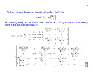

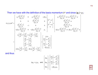
![kjikjip ˆ
1
ˆ1
2
ˆ1
2
ˆˆ1
2
ˆ1
2 2
3
23
2
2
2
2
2
2
2
2
2332
2
2
2
2
2
2
2
β
βκκ
γβ
κκ
−
−
+=
−
+=Λ
p
p
p
p
p
p
p
p
p
p
−−−−++++−−−−++++
Finally we get the eigenvector for the boosted momentum Λp:
k
v
v
jipp
v
ˆ
1
ˆ1
1
2
1ˆ1
1
2
1
1
2
2
22
2
22
2
2
2
0 p
c
c
p
p
p
p
c
p
p
−
−
−=Λ≡
−
≡Λ Λ −−−−++++
κκ
and
so that the four-vector (Λp)µ is given by:
x
Λ3(v)
L2(p)
W−1(Ω)
y
z
We see that the effect of a Lorentz boost L2(p) on the initial unit
momentum p2 followed by a Lorentz transformation Λ3(v) which
has the effect of creating (as seen from O) two component
vectors p1 and p2, magnitudes being equal to ½[1−1/(p2 /κ)2]p2, in
the positive 1- and 2-axis directions and a momentum vector p3 in
the negative 3-axis direction:p2
2
2
3
1
p
c
c
p
−
−=
v
v
The effect of the Wigner rotation W(Λ,p) will produce a rotation
(negative in this case) around the 1-axis which results in an angle
Ω between the 2-axis but also some dispersion resulting in the
overall boost vector Λp ≡p1 i ++++ p2 j −−−−p3 k.
ˆ
ˆ
ˆ ˆ
p3ˆ
ˆ
Suppose that observer O sees a photon with
momentum p in the y-direction and polarization
vector in the z-direction. A second observer O
moves relative to the first with velocity v in the
z-direction. How does O describe the same
photon?
ˆ
ˆˆ
2017
MRT
Λpˆ ≈≈≈≈
p2ˆ
p1ˆ
Ω
116](https://image.slidesharecdn.com/linked-inslides-qft-130507130813-phpapp02/85/Part-IV-Quantum-Fields-116-320.jpg)

![2017
MRT
We finally obtain for the boost matrix L3××××2 (Λp) as a function of the deflection angle Ω:
Ω+Ω
−
Ω+Ω
−
−
+
−
−
−
Ω−Ω
+
Ω
−
−Ω−Ω
−+
=Λ
cossin
2
1)(
sincos
2
1)(
0
2
1)(
001
2
1)(
coscos
2
1)(
00
sin
2
1)(
sincos
2
1)(
0
2
1)(
)(
3
2
2
2
333
2
2
2
33
2
2
2
33
2
2
2
33
2
2
2
2
2
2
333
2
2
2
3
2
2
2
3
23
γ
κ
κ
γβγ
κ
κ
γβ
κ
κ
γβ
κ
κ
γβ
κ
κ
κ
κ
γγβ
κ
κ
γ
κ
κ
γ
p
p
p
p
p
p
p
p
p
p
p
p
p
p
p
p
pL ××××
Ω
−
−=Ω−
Ω+Ω
−
−=
cos
2
1)(
sin
sincos
2
1)(
0
2
2
2
333
3
2
2
2
33
κ
κ
γβγ
γ
κ
κ
γβ
p
p
p
p
−
=Ω⇒
−
=Ω
κ
κ
κ
κ
2
2
2
2
2
2
1
2
1
arctan
1
2
1
tan
p
p
cp
p
c
vv
Since L3××××2 (Λp) is symmetric we can ‘extract’ the [L3××××2 (Λp)]3
2=[L3××××2 (Λp)]2
3 components:
and we obtain:
118
So with only the ratio p2 /κ and |v| we can calculate the photon’s relativistic deflection.](https://image.slidesharecdn.com/linked-inslides-qft-130507130813-phpapp02/85/Part-IV-Quantum-Fields-118-320.jpg)
![Finally, by using the same trigonometric identities relating tanΩ to cosΩ and/or sinΩ:
Ω
Ω+
=Ω
Ω+
=Ω
tan
tan1
sin
tan1
1
cos
2
2
and
such that the boost matrix becomes:
Ω+
+
Ω
Ω+−
Ω
Ω+
+
Ω+
−
−
+
−
−
−
Ω+
−
Ω+
+
Ω
Ω+−
−
Ω
Ω+
−
Ω+
−+
=Λ
2
3
2
2
2
2
33
2
3
2
2
2
2
33
2
2
2
33
2
2
2
2
33
22
2
2
2
2
2
2
3
2
33
2
2
2
2
3
2
2
2
3
23
tan1
1
tan
tan1
2
1)(
tan
tan1
tan1
1
2
1)(
0
2
1)(
001
2
1)(
tan1
1
tan1
1
2
1)(
00
tan
tan1
2
1)(
tan
tan1
tan1
1
2
1)(
0
2
1)(
)(
γ
κ
κ
γβγ
κ
κ
γβ
κ
κ
γβ
κ
κ
γβ
κ
κ
κ
κ
γγβ
κ
κ
γ
κ
κ
γ
p
p
p
p
p
p
p
p
p
p
p
p
p
p
p
p
pL ××××
2017
MRT
We can now either use the relation Ω=arctan{½(|v|/c)[( p2/κ)2 −1]/(p2/κ)} or the one
above by using tanΩ and its square, with p2/κ and β3=|v|/c given beforehand to calculate
things.
119](https://image.slidesharecdn.com/linked-inslides-qft-130507130813-phpapp02/85/Part-IV-Quantum-Fields-119-320.jpg)
![The Klein-Gordon Equation
When Schrödinger wrote down the non-relativistic equation (i.e., ih∂t|ΨΨΨΨ〉=(h2 /2m)|ΨΨΨΨ〉)
now bearing his name, he formulated the corresponding relativistic equation. The
equation is derived by inserting the operator substitution E → ih∂t and p →−ih∇∇∇∇r (with
p=[E/c,p]=ih∂µ where ∂µ =∂/∂xµ ={∂/∂ct,∇∇∇∇} and ∂µ =∂/∂xµ ={∂/∂ct,−∇∇∇∇}) into the
relativistic relation between energy and momentum for a free particle:
where mo is the rest mass of the particle. We then obtain the Klein-Gordon equation:
2017
MRT
42
o
222
cmcE += p
where the d’Alembertian operator is defined as =(1/c2)∂2/∂t2 −∇2 =Σµν ηµν ∂µ ∂ν =Σµ∂µ ∂µ.
The amplitude ϕ is a one-component scalar quantity which under an inhomogeneous
Lorentz transformation, xµ =Λµ
ν xν +aµ, transforms as ϕ (x)=ϕ (x) or equivalently as
ϕ (x) =ϕ [Λ−1(x−a)].
In natural units (i.e., h≡c≡1) and the Dirac notation ϕ (x)=〈x|ϕ〉 with x =xµ =[t,r], we get:
),()(
),( 42
o
2222
tcmc
t
t
r
r
ϕ
ϕ
+∇−=
∂
∂
− hh
0)( 2
o =+ ϕxm
120](https://image.slidesharecdn.com/linked-inslides-qft-130507130813-phpapp02/85/Part-IV-Quantum-Fields-120-320.jpg)

![The Dirac Equation
The Dirac equation has special importance because it describes particles of spin-½,
and both electrons and protons have spin-½. Many other elementary particles, including
the neutron, the µ meson, &c., have spin-½.
In 1928, Dirac discovered the relativistic equation which now bears his name while trying
to overcome the difficulties of negative probability densities of the Klein-Gordon
equation.
2017
MRT
(where =∂2/∂t2 +∇2) if it is to describe a free particle of rest mass mo, since this equation
implies that the energy momentum relation for a free particle p2 =mo
2c2 is satisfied,
and that in the correspondence limit, classical relativity still remains a valid concept.
The reasoning which led Dirac to the Dirac equation was as follows: If we wish to
prevent the occurrence of negative probabilities densities, we must then avoid
time derivatives in the expression for the probability density ρ. The wave equation
must therefore not contain time derivatives higher than first order. Relativistic
covariance, furthermore, requires that there be essentially complete symmetry in the
treatment of the spatial and time components. We must therefore also require that only
first-order spatial derivatives appear in the wave equation. Thus the Dirac wave function
must satisfy a first-order linear differential equation in all four x≡xµ =[t,r] coordinates.
The linearity is required in order that the superposition principle of quantum mechanics
hold. Finally, we must also require ψ(x) that obey the equation:
0)(2
22
o
=
+ x
cm
ψ
h
122](https://image.slidesharecdn.com/linked-inslides-qft-130507130813-phpapp02/85/Part-IV-Quantum-Fields-122-320.jpg)

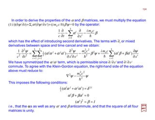


![In terms of the γ matrices, the equation −ihβ∂0ψ −ihΣiβαi∂iψ +mo cψ =0 now reads:
2017
MRT
pγ •−===⋅=/
00
ppppp γγγγ µ
µµ
µ
where γµ is defined by γµ =ηµν γν . With this notation, natural units (i.e., h≡c≡1) and the
Dirac notation ψ (x)=〈x|ψ〉 with x ≡xµ =[t,r], we get:
0oo
=
+•−=
+∂− ψψγ µ
µ
hh
cm
i
cm
i ∂∂∂∂γ
Feynman has introduced the so-called ‘slash’ notation to simplify the equation even
further. For example, he denoted by p the ‘reduced’ quantity:
0)( o =+∂/− ψxcmi
where ∂≡γ µ ∂µ =γ 0 ∂0 +γγγγ •∇∇∇∇.
where our summation convention has been reintroduced. With this last equation, we
have written the Dirac equation in a covariant form where space and time derivatives are
treated alike.
127](https://image.slidesharecdn.com/linked-inslides-qft-130507130813-phpapp02/85/Part-IV-Quantum-Fields-127-320.jpg)
![The Dirac equation (cαααα•p+βmo c2)ψ =Eψ may also be written in two-component form
by means of the Pauli spin matrices:
2017
MRT
where
so that in place of the 4 coupled equations we have:
With σσσσ =[σx,σy,σz] it is seen that
and the 2×2 identity matrix:
−
=
−
=
=
10
01
0
0
01
10
zyx
i
i
σσσ and,
=
10
01
I
−
=
=
I
I
0
0
0
0
βand
σσσσ
σσσσ
αααα
0)(
0)(
2
o
2
o
=+−•
=−+•
vu
uv
Ecmc
Ecmc
ψψ
ψψ
p
p
σσσσ
σσσσ
=
=
4
3
2
1
ψ
ψ
ψ
ψ
ψ
ψ vu and
129](https://image.slidesharecdn.com/linked-inslides-qft-130507130813-phpapp02/85/Part-IV-Quantum-Fields-129-320.jpg)

![Further ψu=[(σσσσ•p)(σσσσ•p)/2mo]ψu reduction of equation is possible with the aid of the
identity (σσσσ•A)(σσσσ•B)=(A•B)+iσσσσ•(A××××B) (which is easily verified from the definitions of
the Pauli matrices – See Landau-Lifshitz Quantum Mechanics). Therefore:
2017
MRT
2
))(( p=•• pp σσσσσσσσ
or, with p=−ih∇∇∇∇:
This equation is still in two-component form since ψu is a two-component function. But
each component of ψu satisfies this equation too so that we can drop all subscripts and
write:
and, substituting in ψu=[(σσσσ•p)(σσσσ•p)/2mo]ψu we get:
uu
m
p
E ψψ
o
2
2
=′
uu
m
E ψψ 2
o
2
2
∇−=′
h
ψψ 2
o
2
2
∇−=′
m
E
h
which is the time-independent Schrödinger equation for a free particle.
131](https://image.slidesharecdn.com/linked-inslides-qft-130507130813-phpapp02/85/Part-IV-Quantum-Fields-131-320.jpg)
![The states of positive energy and spin ±½ are represented by the solutions u1 =
col[1 0 0 0] and u2=col[0 1 0 0] whereas the states of negative energy and spin ±½ are
represented by the solutions u3=col[0 0 1 0] and u4 =col[0 0 0 1].
2017
MRT
2
o
0
3
2
o
0
3 1
2
0
1
1
0
0
0
1
0
0
0
0
1
cmpcmp
uu
=
−=Σ
=
+=Σ
=
= γγ and
which shows that antifermions (i.e., positrons) have negative parity.
Using a parity transformation such that γ 0ψ (t,−r)=ψ (t,r), we get:
2
o
0
3
2
o
0
3 1
4
0
1
3
0
1
0
0
0
0
1
0
0
cmpcmp
uu
−=
−=Σ
−=
+=Σ
−
=
−
= γγ and
which shows that fermions (i.e., electrons, protons, neutrons) have positive parity
whereas:
132](https://image.slidesharecdn.com/linked-inslides-qft-130507130813-phpapp02/85/Part-IV-Quantum-Fields-132-320.jpg)
![We are now in a position to investigate the Lorentz invariance of the Dirac equation
and to establish its connection with the representation of the inhomogeneous Lorentz
group. Under an inhomogeneous Lorentz transformation xµ =Λµ
ν xν +aµ with ηµν Λµ
ρ Λν
σ=
ηρσ the Dirac equation will be form-invariant if we define:
and if S(Λ) satisfies the condition S(Λ)−1γ λ S(Λ)=Λλ
µγ µ ; S(Λ) is a 4×4 matrix which
operates on the components of ψ, i.e., the equation above written explicitly reads:
2017
MRT
Let us now exhibit the actual form of S for a given Lorentz transformation. For the
infinitesimal Lorentz transformation Λ=1 +ελ, xµ =xµ +ελ µ
ν xν (λ µν =−λνµ ), we write
S(Λ) to first order in ε as follows: S(1 +ελ)=1 +εT and [S(1 +ελ)]−1=S−1(1 +ελ)=1 −εT.
For the infinitesimal situations, the equation S(Λ)−1γ λ S(Λ)=Λλ
µγ µ can be rewritten as:
where ∂µ =∂/∂xµ . Note that the γ matrices remainunalteredunderLorentz transformation.
The form-invariance of the Dirac equation is the statement that in the new frame ψ
obeys the equation:
)]([)()()()( 1
axSxSx −ΛΛ=Λ= −
ψψψ
∑=
−
−ΛΛ=
4
1
1
)]([)()(
β
βαβα ψψ axSx
0)()( o =+∂− xcmi ψγ µ
µ
ν
ν
µµν
ν
µµµµµµ
γλεγγγγεγεγεγ +=Λ=−+=+−=−
)()1()1(1
TTTTSS
where T must be such that γ µ T− Tγ µ =λµ
ν γν and is given by T =(1/8)λµν (γµ γν − γν γµ ).
133](https://image.slidesharecdn.com/linked-inslides-qft-130507130813-phpapp02/85/Part-IV-Quantum-Fields-133-320.jpg)
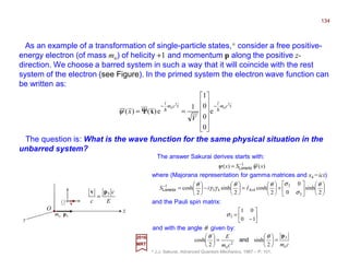
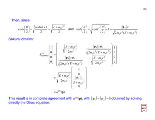
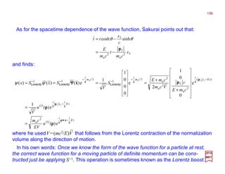
(
)(),(),(
1
axS
xaUxaUx
−ΛΛ=
Λ==Λ
−
ψ
ψψψ
ψψ =Λ ),( aU
=≡
0
0
i
i
i
σ
σ
ααααα
1
1
1
322
1
1 Σ
20
0
)(
ii
RT +=
+=−=
σ
σ
αα
h
137](https://image.slidesharecdn.com/linked-inslides-qft-130507130813-phpapp02/85/Part-IV-Quantum-Fields-137-320.jpg)
![where D, the infinitesimal generator, is determined by using equations xµ =xµ +ελ µ
ν xν
and S(1 +ελ)=1 +εT by equation 〈x|U(Λ,a)|ψ〉=〈x |ψ 〉=U(Λ,a)ψ(x)=S(Λ)ψ [Λ−1(x−a)]:
For an infinitesimal quantum transformation, we write:
2017
MRT
D
i
aU ε
h
+=Λ 1),(
For an infinitesimal rotation about the 3-axis, T=½iΣ3 and only λ21 =−λ12 =+1 are
different from zero, so that:
Thus, a Dirac particle has in addition to its orbital momentum, r××××p, an intrinsic angular
momentum ΣΣΣΣ of magnitude h/2. It is to be noted that the spin operator ½ΣΣΣΣ is not a
constant of motion, since [H,ΣΣΣΣ]≠0.The same is true for the orbital angular momentum;
however, the total angular momentum J=(h/2)ΣΣΣΣ++++(r××××p) is a constant of the motion.
so that
3323 )(Σ pr ××××+= hD
)( ρ
σ
σ
ρ
λ ∂−−= xTiD h
L
L
h
+∂−+=
+
∂
∂
−+=
−+=
+
)()()(
)(
)()()1(
)()1(1
xxTx
x
x
xxT
xxTD
i
ψλεψ
ψ
λεψε
λεψεε
µ
ν
ν
µ
µ
µ
138](https://image.slidesharecdn.com/linked-inslides-qft-130507130813-phpapp02/85/Part-IV-Quantum-Fields-138-320.jpg)
![We now consider the Dirac equation with electromagnetic coupling.
in which v is the velocity of a particle with positive charge q and rest mass mo, A and ϕ
are the vector and scalar potentials, respectively. The fields are then given by:
2017
MRT
ϕq
c
q
vmL −•+= Av2
o
2
1
It will now be assumed that the same modification can be introduced into the free-
particle Dirac equation (cαααα•p+βmo c2)ψ =Eψ so that the proper equation for a particle in
a field with vector potential A and scalar potential ϕ is:
ϕ∇∇∇∇××××∇∇∇∇ −
∂
∂
−==
tc
A
EAB
1
and
ψϕβψ ])([ 2
o qcmqcE ++−•= Apαααα
In two-component form, by analogy to the equations cσσσσ•pψv+(moc2 −E)ψu=0 and
cσσσσ•pψu−(moc2 +E)ψv =0, we set:
vvu
uuv
Eqcmqc
Eqcmqc
ψψϕψ
ψψϕψ
=−−−•
=++−•
)()(
)()(
2
o
2
o
Ap
Ap
σσσσ
σσσσ
The free-particle Dirac equation (cαααα•p+βmo c2)ψ =Eψ must now be modified to
include effects due to external fields. Classical considerations suggest how this may be
accomplished. In the presence of external fields a possible Lagrangian for the system is:
139](https://image.slidesharecdn.com/linked-inslides-qft-130507130813-phpapp02/85/Part-IV-Quantum-Fields-139-320.jpg)
![2017
MRT
The identity (σσσσ•A)(σσσσ•B)=(A•B)+iσσσσ•(A××××B) gives (σσσσ•A)2 =ππππ2 +iσσσσ•(ππππ××××ππππ)=[p−(q/c)A]2 −
i(q/c)σσσσ•(p××××A++++A××××p). But p××××A=−ih∇∇∇∇××××A−A××××p, therefore we get:
As in the free particle case, we shall be interested mainly in the ‘large’ component ψu.
From the equations σσσσ•(cp−−−−qA)ψv+(moc2 +qϕ)ψu=Eψu and σσσσ•(cp−−−−qA)ψu−(moc2 −qϕ)ψv=
Eψv, we set:
where
Our objective now is to obtain an approximation to the equation above to order v2/c2.
Ap
c
q
cmqEqcmE
cm
KcmEE −=
−′+
=
−+′
=−=′ ππππand,
]2/)[(1
1
2
2
2
o
2
o
2
o2
o
ϕϕ
uu K
m
qE ψψϕ )()(
2
1
)(
o
ππππσσσσππππσσσσ ••=−′
uu
cm
q
c
q
m
qE ψψϕ
•−
−=−′ AAp ××××∇∇∇∇σσσσ
o
2
o 22
1
)(
h
and the approximation to (E′− qϕ)ψu=(1/2mo)(σσσσ•ππππ)K(σσσσ•ππππ)ψu with K=1 is:
AAp ××××∇∇∇∇σσσσππππσσσσ •−
−=•
cm
q
c
q
o
2
2
2
)(
h
140](https://image.slidesharecdn.com/linked-inslides-qft-130507130813-phpapp02/85/Part-IV-Quantum-Fields-140-320.jpg)
![2017
MRT
Substitution of the above simplification into the equation (E′−qϕ)ψ = […]ψ above gives:
Therefore:
Hence, the transformed equation Ω−1(E′−qϕ)Ω−1ψu, to order v2/c2, becomes:
A number of simplifications are possible with the aid of:
ψϕϕ
ϕψϕ
•
−′+•−′•−
−′
•
+•−•=−′
22
o
2
22
o
22
o
2
4
23
o
2
o
8
)(
)())()((
4
1
)(
8
)(
)(
8
1
)(
2
1
)(
cm
qEqE
cm
qE
cmcmm
qE
ππππσσσσ
ππππσσσσππππσσσσ
ππππσσσσ
ππππσσσσππππσσσσ
ϕϕϕϕ
ϕϕϕϕϕ
∇∇∇∇××××ππππσσσσ∇∇∇∇∇∇∇∇ππππσσσσ∇∇∇∇σσσσ∇∇∇∇σσσσππππσσσσ
∇∇∇∇σσσσσσσσσσσσππππσσσσππππσσσσ
•+•−=••−••
•=•−•=•−′−−′•
ii
qiqqqEqE
2))(())((
)())(())((
h
hpp
))()((22
))()((2))]()(())([(
)])(())()[(())(()()(
2
22
ππππσσσσππππσσσσ∇∇∇∇××××ππππσσσσ∇∇∇∇∇∇∇∇
ππππσσσσππππσσσσππππσσσσππππσσσσππππσσσσ
ππππσσσσππππσσσσππππσσσσππππσσσσππππσσσσ
•−′•+•−•=
•−′•+••−′−−′•−
−•−′−−′••=•−′+−′•
ϕϕϕ
ϕϕϕ
ϕϕϕϕ
qEqq
qEqEqE
qEqEqEqE
hh
ψϕϕψϕ
•−•+•−•=−′ ∇∇∇∇××××ππππσσσσ∇∇∇∇∇∇∇∇ππππσσσσππππσσσσ 22
o
22
o
2
4
23
o
2
o 48
)(
8
1
)(
2
1
)(
cm
q
cm
q
cmm
qE
hh
142](https://image.slidesharecdn.com/linked-inslides-qft-130507130813-phpapp02/85/Part-IV-Quantum-Fields-142-320.jpg)
![Also, from the relation (σσσσ•A)2 =[p–(q/c)A]2−(qh/c)σσσσ•∇∇∇∇××××A obtained earlier, we get:
and, to order v2/c2, we finally have:
2017
MRT
ppp ××××∇∇∇∇))))××××∇∇∇∇∇∇∇∇××××∇∇∇∇∇∇∇∇××××∇∇∇∇××××ππππ
ππππσσσσ
ϕϕϕϕϕ 2222
4
4
4
2
1
(
111
)(
1
c
i
ccc
c
p
c
−=−−==
=•
h
AAp ××××∇∇∇∇σσσσππππσσσσ •−
−=•
cm
q
c
q
mm o
2
o
2
o 22
1
)(
2
1 h
where E′=E−moc2. This equation, which may be regarded as the Schrödinger equation
for an electron interacting with fields describable by the potentials A and ϕ, is the
starting point for discussions of atomic and molecular properties.
With q =−e, where e is the electronic charge, we obtain for an electron to order v2/c2:
ψϕϕ
ψϕ
•−•−−
−•+
+=+′
p
AAp
××××∇∇∇∇σσσσ∇∇∇∇∇∇∇∇
××××∇∇∇∇σσσσ
22
o
22
o
2
23
o
4
o
2
o
488
22
1
)(
cm
e
cm
e
cm
p
cm
e
c
e
m
eE
hh
h
143](https://image.slidesharecdn.com/linked-inslides-qft-130507130813-phpapp02/85/Part-IV-Quantum-Fields-143-320.jpg)
![This is the energy associated with the scalar potential energy, ϕ (105 cm−1).
This significance of the various terms and their energies, indicated to within an order of
magnitude, are (the ‘cm−1’ scale is given by the wave number 1/λ ≅ 8000 cm−1):
This contains the kinetic energy (i.e., p2 /2mo) and interaction term (i.e., (e/2moc)(p • A + A• p)
+ e2A2/2moc2) with a field represented by a potential vector A (105 cm−1). The interaction terms
are responsible or contribute to numerous physical processes among which are absorption,
emission and scattering of electromagnetic waves, diamagnetism, and the Zeeman effect.
2017
MRT
ϕe
The spin-orbit interaction (10-103 cm−1). More precisely, itis (eh/8moc2){σσσσ •[p −−−− (e/c)A]×××× E −−−−
σσσσ • E ×××× [p −−−− (e/c)A]} and it arises from the fact that the motion of the magnetic moment gives
rise to an electric moment for the particle which then interacts with the electric field.
This term appears in the expression of the relativistic energy:
and is therefore a relativistic correction to the kinetic energy (i.e., p2/2m) (0.1 cm−1).
The interaction of the spin magnetic moment (i.e., µS = 2⋅e/2mo⋅h/2) with a magnetic field B=
∇∇∇∇ ×××× A (1 cm−1). Thus, it is the magnetic moment of one Bohr magneton, eh/2moc
(i.e., µB = 9.2741×10⁻²⁴ A⋅m2 or J/T) with the magnetic field.
2
o2
1
+ Ap
c
e
m
A××××∇∇∇∇σσσσ •
cm
e
o2
h
23
o
4
8 cm
p
L+−+≅+ 23
o
2
2
o
2222
o
82
)(
cm
p
m
p
cmcpcm
4
ϕ∇∇∇∇∇∇∇∇ •− 22
o
2
8 cm
eh
This term produces an energy shift in s-states and is known as the Darwin (1887-1962) term
(< 0.1 cm−1). It is thus a correction to the direct point charge interaction due to the fact that in the
representation (Foldy-Wouthuysen), the particle is not concentrated at a point but is spread out
over a volume with radius whose magnitude is roughly that of a Compton wavelength, h/moc.
p××××∇∇∇∇σσσσ ϕ•− 22
o4 cm
eh
ϕe
c
e
m
−
+
2
o2
1
Ap
As a combination, this term represents the interaction of a point charge with the
electromagnetic field.
144](https://image.slidesharecdn.com/linked-inslides-qft-130507130813-phpapp02/85/Part-IV-Quantum-Fields-144-320.jpg)
![The solution in the Coulomb field has important applications, particularly to the energy
levels of the hydrogen atom and to the calculation of x-ray spectra due to the K and L
electrons of the heavy elements.
2017
MRT
In the general case of hydrogen-like atoms (e.g., the Hydrogen atom H1 has Z=1), the
energy levels En j are described by the total angular momentum quantum number j with:
2222
22
2
o
])½([
1
Zjn
Z
cmE jn
α
α
−++′
+=
where n′=0,1,2,….; j =1/2,3/2,…; α =e2/4πhc ≅1/137 and can be approximated by:
+
−
+
+−≈ L
njn
Z
n
Z
cmcmE jn
4
3
½
1
1
2
1 2
2
22
2
o
22
o
α
α
and where the principle quantum number n = n′+j +½ =1,2,….
The observed fine structure of the levels of hydrogen and hydrogen-like atoms,
particularly Helium He+, is in good agreement with the Dirac theory. FIN
The atomic number is the number of protons found in the nucleus of an atom and
therefore identical to the charge number of the nucleus. It is conventionally represented
by the symbol Z. The atomic number uniquely identifies a chemical element. In an atom
of neutral charge, the atomic number is also equal to the number of electrons.
145](https://image.slidesharecdn.com/linked-inslides-qft-130507130813-phpapp02/85/Part-IV-Quantum-Fields-145-320.jpg)

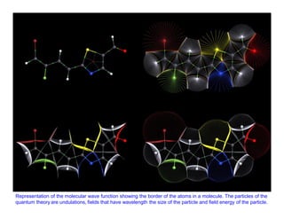


The document summarizes key concepts from quantum mechanics and symmetries. It states that physical states are represented by rays in a Hilbert space, with observables represented by Hermitian operators. The probability of measuring a state is given by the inner product of the state vectors. Symmetries are represented by either unitary or antiunitary operators on the Hilbert space. Symmetries that can be continuously connected to the identity must be represented by unitary operators. Symmetries form a group, with transformations combining according to the group multiplication rule.


