This lecture discusses operator methods in quantum mechanics. Some key points: 1. Operators allow quantum mechanics to be formulated without relying on a particular basis. The Hamiltonian operator H acts on state vectors. 2. Dirac notation represents state vectors as "kets" and defines inner products between states. A resolution of identity allows expanding states in a basis. 3. Hermitian operators correspond to physical observables. Their eigenfunctions form a complete basis. The time-evolution operator evolves states forward in time. 4. The uncertainty principle relates the uncertainties of non-commuting operators like position and momentum. Symmetries of the Hamiltonian are represented by unitary operators that commute with it.

1. Lecture 3
Operator methods in quantum mechanics

2. Background
Although wave mechanics is capable of describing quantum
behaviour of bound and unbound particles, some properties can not
be represented this way, e.g. electron spin degree of freedom.
It is therefore convenient to reformulate quantum mechanics in
framework that involves only operators, e.g. ˆH.
Advantage of operator algebra is that it does not rely upon
particular basis, e.g. for ˆH = ˆp2
2m , we can represent ˆp in spatial
coordinate basis, ˆp = −i ∂x , or in the momentum basis, ˆp = p.
Equally, it would be useful to work with a basis for the
wavefunction, ψ, which is coordinate-independent.

3. Operator methods: outline
1 Dirac notation and definition of operators
2 Uncertainty principle for non-commuting operators
3 Time-evolution of expectation values: Ehrenfest theorem
4 Symmetry in quantum mechanics
5 Heisenberg representation
6 Example: Quantum harmonic oscillator
(from ladder operators to coherent states)

4. Dirac notation
Orthogonal set of square integrable functions (such as
wavefunctions) form a vector space (cf. 3d vectors).
In Dirac notation, state vector or wavefunction, ψ, is represented
symbolically as a “ket”, |ψ .
Any wavefunction can be expanded as sum of basis state vectors,
(cf. v = xˆex + yˆey + · · · )
|ψ = λ1|ψ1 + λ2|ψ2 + · · ·
Alongside ket, we can define a “bra”, ψ| which together form the
scalar product,
φ|ψ ≡
∞
−∞
dx φ∗
(x)ψ(x) = ψ|φ ∗

5. Dirac notation
For a complete basis set, φi , we can define the expansion
|ψ =
i
φi |i
where j|ψ =
i
φi j|i
δij
= φj .
For example, in the real space basis, |ψ = dx ψ(x)|x .
Then, since x|x = δ(x − x ),
x |ψ = dx ψ(x) x |x
δ(x−x )
= ψ(x )
In Dirac formulation, real space representation recovered from inner
product, ψ(x) = x|ψ ; equivalently ψ(p) = p|ψ .

6. Operators
An operator ˆA maps one state vector, |ψ , into another, |φ , i.e.
ˆA|ψ = |φ .
If ˆA|ψ = a|ψ with a real, then |ψ is said to be an eigenstate (or
eigenfunction) of ˆA with eigenvalue a.
e.g. plane wave state ψp(x) = x|ψp = A eipx/
is an eigenstate of
the momentum operator, ˆp = −i ∂x , with eigenvalue p.
For every observable A, there is an operator ˆA which acts upon the
wavefunction so that, if a system is in a state described by |ψ , the
expectation value of A is
A = ψ|ˆA|ψ =
∞
−∞
dx ψ∗
(x)ˆAψ(x)

7. Operators
Every operator corresponding to observable is linear and Hermitian,
i.e. for any two wavefunctions |ψ and |φ , linearity implies
ˆA(α|ψ + β|φ ) = α ˆA|ψ + β ˆA|φ
For any linear operator ˆA, the Hermitian conjugate (a.k.a. the
adjoint) is defined by relation
φ|ˆAψ = dx φ∗
(ˆAψ) = dx ψ(ˆA†
φ)∗
= ˆA†
φ|ψ
Hermiticity implies that ˆA†
= ˆA, e.g. ˆp = −i ∂x .

8. Operators
From the definition, ˆA†
φ|ψ = φ|ˆAψ , some useful relations follow:
1 From complex conjugation, ˆA†
φ|ψ ∗
= ψ|ˆA†
φ = ˆAψ|φ ,
i.e. (ˆA†
)†
ψ|φ = ˆAψ|φ , ⇒ (ˆA†
)†
= ˆA
2 From φ|ˆAˆBψ = ˆA†
φ|ˆBψ = ˆB† ˆA†
φ|ψ ,
it follows that (ˆAˆB)†
= ˆB† ˆA†
.
Operators are associative,i.e. (ˆAˆB)ˆC = ˆA(ˆB ˆC),
but not (in general) commutative,
ˆAˆB|ψ = ˆA(ˆB|ψ ) = (ˆAˆB)|ψ = ˆB ˆA|ψ .

9. Operators
A physical variable must have real expectation values (and
eigenvalues) ⇒ physical operators are Hermitian (self-adjoint):
ψ|ˆH|ψ ∗
=
∞
−∞
ψ∗
(x)ˆHψ(x)dx
∗
=
∞
−∞
ψ(x)(ˆHψ(x))∗
dx = ˆHψ|ψ
i.e. ˆHψ|ψ = ψ|ˆHψ = ˆH†
ψ|ψ , and ˆH†
= ˆH.
Eigenfunctions of Hermitian operators ˆH|i = Ei |i form complete
orthonormal basis, i.e. i|j = δij
For complete set of states |i , can expand a state function |ψ as
|ψ =
i
|i i|ψ
In coordinate representation,
ψ(x) = x|ψ =
i
x|i i|ψ =
i
i|ψ φi (x), φi (x) = x|i

10. Resolution of identity
|ψ =
i
|i i|ψ
If we sum over complete set of states, obtain the (useful) resolution
of identity,
i
|i i| = I
i
x |i i|x = x |x
i.e. in coordinate basis, i φ∗
i (x)φi (x ) = δ(x − x ).
As in 3d vector space, expansion |φ = i bi |i and |ψ = i ci |i
allows scalar product to be taken by multiplying components,
φ|ψ = i b∗
i ci .

11. Example: resolution of identity
Basis states can be formed from any complete set of orthogonal
states including position or momentum,
∞
−∞
dx|x x| =
∞
−∞
dp|p p| = I.
From these definitions, can recover Fourier representation,
ψ(x) ≡ x|ψ =
∞
−∞
dp x|p
eipx/
/
√
2π
p|ψ =
1
√
2π
∞
−∞
dp eipx/
ψ(p)
where x|p denotes plane wave state |p expressed in the real space
basis.

12. Time-evolution operator
Formally, we can evolve a wavefunction forward in time by applying
time-evolution operator.
For time-independent Hamiltonian, |ψ(t) = ˆU(t)|ψ(0) , where
time-evolution operator (a.k.a. the “propagator”):
ˆU(t) = e−i ˆHt/
follows from time-dependent Schr¨odinger equation, ˆH|ψ = i ∂t|ψ .
By inserting the resolution of identity, I = i |i i|, where |i are
eigenstates of ˆH with eigenvalue Ei ,
|ψ(t) = e−i ˆHt/
i
|i i|ψ(0) =
i
|i i|ψ(0) e−iEi t/

13. Time-evolution operator
ˆU = e−i ˆHt/
Time-evolution operator is an example of a Unitary operator:
Unitary operators involve transformations of state vectors which
preserve their scalar products, i.e.
φ|ψ = ˆUφ|ˆUψ = φ|ˆU† ˆUψ
!
= φ|ψ
i.e. ˆU† ˆU = I

14. Uncertainty principle for non-commuting operators
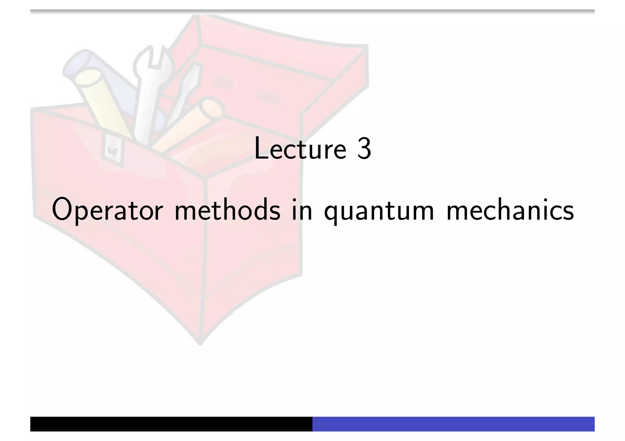
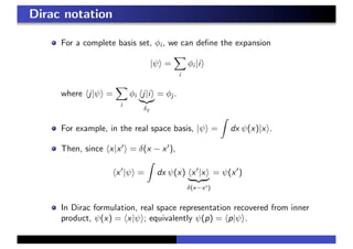
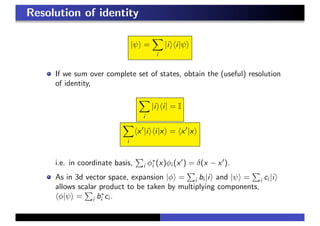
For non-commuting Hermitian operators, we can establish a bound
on the uncertainty in the expectation values of ˆA and ˆB:
Given a state |ψ , the mean square uncertainty defined as
(∆A)2
= ψ|(ˆA − ˆA )2
ψ = ψ|ˆU2
ψ
(∆B)2
= ψ|(ˆB − ˆB )2
ψ = ψ| ˆV 2
ψ
where ˆU = ˆA − ˆA , ˆA ≡ ψ|ˆAψ , etc.
Consider then the expansion of the norm ||ˆU|ψ + iλ ˆV |ψ ||2
,
ψ|ˆU2
ψ + λ2
ψ| ˆV 2
ψ + iλ ˆUψ| ˆV ψ − iλ ˆV ψ|ˆUψ ≥ 0
i.e. (∆A)2
+ λ2
(∆B)2
+ iλ ψ|[ˆU, ˆV ]|ψ ≥ 0
Since ˆA and ˆB are just constants, [ˆU, ˆV ] = [ˆA, ˆB].

15. Uncertainty principle for non-commuting operators
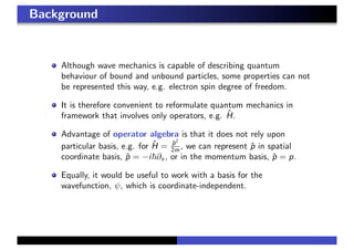
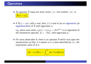
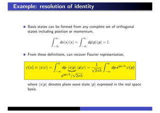
(∆A)2
+ λ2
(∆B)2
+ iλ ψ|[ˆA, ˆB]|ψ ≥ 0
Minimizing with respect to λ,
2λ(∆B)2
+ iλ ψ|[ˆA, ˆB]|ψ = 0, iλ =
1
2
ψ|[ˆA, ˆB]|ψ
(∆B)2
and substituting back into the inequality,
(∆A)2
(∆B)2
≥ −
1
4
ψ|[ˆA, ˆB]|ψ 2
i.e., for non-commuting operators,
(∆A)(∆B) ≥
i
2
[ˆA, ˆB]

16. Uncertainty principle for non-commuting operators
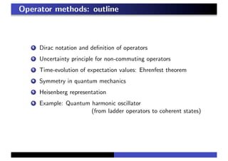
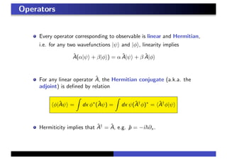
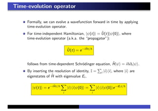
(∆A)(∆B) ≥
i
2
[ˆA, ˆB]
For the conjugate operators of momentum and position (i.e.
[ˆp, ˆx] = −i , recover Heisenberg’s uncertainty principle,
(∆p)(∆x) ≥
i
2
[ˆp, x] =
2
Similarly, if we use the conjugate coordinates of time and energy,
[ˆE, t] = i ,
(∆t)(∆E) ≥
i
2
[t, ˆE] =
2

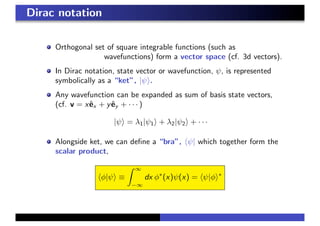
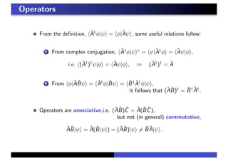
17. Time-evolution of expectation values
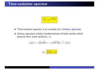
For a general (potentially time-dependent) operator ˆA,
∂t ψ|ˆA|ψ = (∂t ψ|)ˆA|ψ + ψ|∂t
ˆA|ψ + ψ|ˆA(∂t|ψ )
Using i ∂t|ψ = ˆH|ψ , −i (∂t ψ|) = ψ|ˆH, and Hermiticity,
∂t ψ|ˆA|ψ =
1
i ˆHψ|ˆA|ψ + ψ|∂t
ˆA|ψ +
1
ψ|ˆA|(−i ˆHψ)
=
i
ψ|ˆH ˆA|ψ − ψ|ˆAˆH|ψ
ψ|[ˆH, ˆA]|ψ
+ ψ|∂t
ˆA|ψ
For time-independent operators, ˆA, obtain Ehrenfest Theorem,
∂t ψ|ˆA|ψ =
i
ψ|[ˆH, ˆA]|ψ .

18. Ehrenfest theorem: example
∂t ψ|ˆA|ψ =
i
ψ|[ˆH, ˆA]|ψ .
For the Schr¨odinger operator, ˆH = ˆp2
2m + V (x),
∂t x =
i
[ˆH, ˆx] =
i
[
ˆp2
2m
, x] =
ˆp
m
Similarly,
∂t ˆp =
i
[ˆH, −i ∂x ] = − (∂x
ˆH) = − ∂x V
i.e. Expectation values follow Hamilton’s classical equations of
motion.

19. Symmetry in quantum mechanics
Symmetry considerations are very important in both low and high
energy quantum theory:
1 Structure of eigenstates and spectrum reflect symmetry of the
underlying Hamiltonian.
2 Transition probabilities between states depend upon
transformation properties of perturbation =⇒ “selection
rules”.
Symmetries can be classified as discrete and continuous,
e.g. mirror symmetry is discrete, while rotation is continuous.

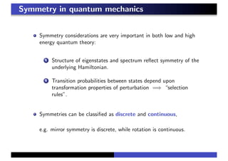
20. Symmetry in quantum mechanics
Formally, symmetry operations can be represented by a group of
(typically) unitary transformations (or operators), ˆU such that
ˆO → ˆU† ˆO ˆU
Such unitary transformations are said to be symmetries of a
general operator ˆO if
ˆU† ˆO ˆU = ˆO
i.e., since ˆU†
= ˆU−1
(unitary), [ ˆO, ˆU] = 0.
If ˆO ≡ ˆH, such unitary transformations are said to be symmetries of
the quantum system.

21. Continuous symmetries: Examples
Operators ˆp and ˆr are generators of space-time transformations:
For a constant vector a, the unitary operator
ˆU(a) = exp −
i
a · ˆp
effects spatial translations, ˆU†
(a)f (r)ˆU(a) = f (r + a).
Proof: Using the Baker-Hausdorff identity (exercise),
e
ˆA ˆBe−ˆA
= ˆB + [ˆA, ˆB] +
1
2!
[ˆA, [ˆA, ˆB]] + · · ·
with e
ˆA
≡ ˆU†
= ea·
and ˆB ≡ f (r), it follows that
ˆU†
(a)f (r)ˆU(a) = f (r) + ai1 ( i1 f (r)) +
1
2!
ai1 ai2 ( i1 i2 f (r)) + · · ·
= f (r + a) by Taylor expansion

22. Continuous symmetries: Examples
Operators ˆp and ˆr are generators of space-time transformations:
For a constant vector a, the unitary operator
ˆU(a) = exp −
i
a · ˆp
effects spatial translations, ˆU†
(a)f (r)ˆU(a) = f (r + a).
Therefore, a quantum system has spatial translation symmetry iff
ˆU(a)ˆH = ˆH ˆU(a), i.e. ˆpˆH = ˆHˆp
i.e. (sensibly) ˆH = ˆH(ˆp) must be independent of position.
Similarly (with ˆL = r × ˆp the angular momemtum operator),



ˆU(b) = exp[− i
b · ˆr]
ˆU(θ) = exp[− i
θˆen · ˆL]
ˆU(t) = exp[− i ˆHt]
effects



momentum translations
spatial rotations
time translations

23. Discrete symmetries: Examples
The parity operator, ˆP, involves a sign reversal of all coordinates,
ˆPψ(r) = ψ(−r)
discreteness follows from identity ˆP2
= 1.
Eigenvalues of parity operation (if such exist) are ±1.
If Hamiltonian is invariant under parity, [ˆP, ˆH] = 0, parity is said to
be conserved.
Time-reversal is another discrete symmetry, but its representation
in quantum mechanics is subtle and beyond the scope of course.

24. Consequences of symmetries: multiplets
Consider a transformation ˆU which is a symmetry of an operator
observable ˆA, i.e. [ˆU, ˆA] = 0.
If ˆA has eigenvector |a , it follows that ˆU|a will be an eigenvector
with the same eigenvalue, i.e.
ˆAU|a = ˆU ˆA|a = aU|a
This means that either:
1 |a is an eigenvector of both ˆA and ˆU (e.g. |p is eigenvector
of ˆH = ˆp2
2m and ˆU = eia·ˆp/
), or
2 eigenvalue a is degenerate: linear space spanned by vectors
ˆUn
|a (n integer) are eigenvectors with same eigenvalue.
e.g. next lecture, we will address central potential where ˆH is
invariant under rotations, ˆU = eiθˆen·ˆL/
– states of angular
momentum, , have 2 + 1-fold degeneracy generated by ˆL±.

25. Heisenberg representation
Schr¨odinger representation: time-dependence of quantum system
carried by wavefunction while operators remain constant.
However, sometimes useful to transfer time-dependence to
operators: For observable ˆB, time-dependence of expectation value,
ψ(t)|ˆB|ψ(t) = e−i ˆHt/
ψ(0)|ˆB|e−i ˆHt/
ψ(0)
= ψ(0)|ei ˆHt/ ˆBe−i ˆHt/
|ψ(0)
Heisenberg representation: if we define ˆB(t) = ei ˆHt/ ˆBe−i ˆHt/
,
time-dependence transferred from wavefunction and
∂t
ˆB(t) =
i
ei ˆHt/
[ˆH, ˆB]e−i ˆHt/
=
i
[ˆH, ˆB(t)]
cf. Ehrenfest’s theorem

26. Quantum harmonic oscillator
The harmonic oscillator holds priviledged position in quantum
mechanics and quantum field theory.
ˆH =
ˆp2
2m
+
1
2
mω2
x2
It also provides a useful platform to illustrate some of the
operator-based formalism developed above.
To obtain eigenstates of ˆH, we could seek solutions of linear second
order differential equation,
−
2
2m
∂2
x +
1
2
mω2
x2
ψ = Eψ
However, complexity of eigenstates (Hermite polynomials) obscure
useful features of system – we therefore develop an alternative
operator-based approach.

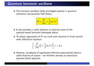
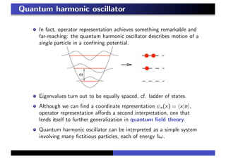
27. Quantum harmonic oscillator
ˆH =
ˆp2
2m
+
1
2
mω2
x2
Form of Hamiltonian suggests that it can be recast as the “square
of an operator”: Defining the operators (no hats!)
a =
mω
2
x + i
ˆp
mω
, a†
=
mω
2
x − i
ˆp
mω
we have a†
a =
mω
2
x2
+
ˆp2
2 mω
−
i
2
[ˆp, x]
−i
=
ˆH
ω
−
1
2
Together with aa†
=
ˆH
ω + 1
2 , we find that operators fulfil the
commutation relations
[a, a†
] ≡ aa†
− a†
a = 1
Setting ˆn = a†
a, ˆH = ω(ˆn + 1/2)

28. Quantum harmonic oscillator
ˆH = ω(a†
a + 1/2)
Ground state |0 identified by finding state for which
a|0 =
mω
2
x + i
ˆp
mω
|0 = 0
In coordinate basis,
x|a|0 = 0 = dx x|a|x x |0 = x +
mω
∂x ψ0(x)
i.e. ground state has energy E0 = ω/2 and
ψ0(x) = x|0 =
mω
π
1/4
e−mωx2
/2
N.B. typo in handout!

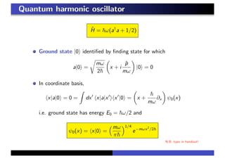
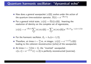
29. Quantum harmonic oscillator
ˆH = ω(a†
a + 1/2)
Excited states found by acting upon this state with a†
.
Proof: using [a, a†
] ≡ aa†
− a†
a = 1, if ˆn|n = n|n ,
ˆn(a†
|n ) = a†
aa†
a†
a + 1
|n = (a†
a†
a
ˆn
+a†
)|n = (n + 1)a†
|n
equivalently, [ˆn, a†
] = ˆna†
− a†
ˆn = a†
.
Therefore, if |n is eigenstate of ˆn with eigenvalue n, then a†
|n is
eigenstate with eigenvalue n + 1.
Eigenstates form a “tower”; |0 , |1 = C1a†
|0 , |2 = C2(a†
)2
|0 , ...,
with normalization Cn.

30. Quantum harmonic oscillator
ˆH = ω(a†
a + 1/2)
Normalization: If n|n = 1, n|aa†
|n = n|(ˆn + 1)|n = (n + 1),
i.e. with |n + 1 = 1√
n+1
a†
|n , state |n + 1 also normalized.
|n =
1
√
n!
(a†
)n
|0 , n|n = δnn
are eigenstates of ˆH with eigenvalue En = (n + 1/2) ω and
a†
|n =
√
n + 1|n + 1 , a|n =
√
n|n − 1
a and a†
represent ladder operators that lower/raise energy of
state by ω.

31. Quantum harmonic oscillator
In fact, operator representation achieves something remarkable and
far-reaching: the quantum harmonic oscillator describes motion of a
single particle in a confining potential.
Eigenvalues turn out to be equally spaced, cf. ladder of states.
Although we can find a coordinate representation ψn(x) = x|n ,
operator representation affords a second interpretation, one that
lends itself to further generalization in quantum field theory.
Quantum harmonic oscillator can be interpreted as a simple system
involving many fictitious particles, each of energy ω.

32. Quantum harmonic oscillator
In new representation, known as the Fock space representation,
vacuum |0 has no particles, |1 a single particle, |2 has two, etc.
Fictitious particles created and annihilated by raising and lowering
operators, a†
and a with commutation relations, [a, a†
] = 1.
Later in the course, we will find that these commutation relations
are the hallmark of bosonic quantum particles and this
representation, known as second quantization underpins the
quantum field theory of relativistic particles (such as the photon).

33. Quantum harmonic oscillator: “dynamical echo”
How does a general wavepacket |ψ(0) evolve under the action of
the quantum time-evolution operator, ˆU(t) = e−i ˆHt/
?
For a general initial state, |ψ(t) = ˆU(t)|ψ(0) . Inserting the
resolution of identity on the complete set of eigenstates,
|ψ(t) = e−i ˆHt/
n
|n n|ψ(0) =
i
|n n|ψ(0) e−iEnt/
e−iω(n+1/2)t
For the harmonic oscillator, En = ω(n + 1/2).
Therefore, at times t = 2π
ω m, m integer, |ψ(t) = e−iωt/2
|ψ(0)
leading to the coherent reconstruction (echo) of the wavepacket.
At times t = π
ω (2m + 1), the “inverted” wavepacket
ψ(x, t) = e−iωt/2
ψ(−x, 0) is perfectly reconstructed (exercise).

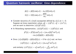
34. Quantum harmonic oscillator: time-dependence
In Heisenberg representation, we have seen that ∂t
ˆB =
i
[ˆH, ˆB].
Therefore, making use of the identity, [ˆH, a] = − ωa (exercise),
∂ta = −iωa, i.e. a(t) = e−iωt
a(0)
Combined with conjugate relation a†
(t) = eiωt
a†
(0), and using
x = 2mω (a†
+ a), ˆp = −i m ω
2 (a − a†
)
ˆp(t) = ˆp(0) cos(ωt) − mωˆx(0) sin(ωt)
ˆx(t) = ˆx(0) cos(ωt) +
ˆp(0)
mω
sin(ωt)
i.e. operators obey equations of motion of the classical harmonic
oscillator.
But how do we use these equations...?

35. Quantum harmonic oscillator: time-dependence
ˆp(t) = ˆp(0) cos(ωt) − mωˆx(0) sin(ωt)
ˆx(t) = ˆx(0) cos(ωt) +
ˆp(0)
mω
sin(ωt)
Consider dynamics of a (real) wavepacket defined by φ(x) at t = 0.
Suppose we know expectation values, p2
0 = φ|ˆp2
|φ , x2
0 = φ|x2
|φ ,
and we want to determine φ(t)|ˆp2
|φ(t) .
In Heisenberg representation, φ(t)|ˆp2
|φ(t) = φ|ˆp2
(t)|φ and
ˆp2
(t) = ˆp2
(0) cos2
(ωt) + (mωx(0))2
sin2
(ωt)
−mω(x(0)ˆp(0) + ˆp(0)x(0))
Since φ|(x(0)ˆp(0) + ˆp(0)x(0))|φ = 0 for φ(x) real, we have
φ|ˆp2
(t)|φ = p2
0 cos2
(ωt) + (mωx0)2
sin2
(ωt)
and similarly φ|ˆx2
(t)|φ = x2
0 cos2
(ωt) +
p2
0
(mω)2 sin2
(ωt)

36. Coherent states
The ladder operators can be used to construct a wavepacket which
most closely resembles a classical particle – the coherent or
Glauber states.
Such states have numerous applications in quantum field theory and
quantum optics.
The coherent state is defined as the eigenstate of the annihilation
operator,
a|β = β|β
Since a is not Hermitian, β can take complex eigenvalues.
The eigenstates are constructed from the harmonic oscillator ground
state the by action of the unitary operator,
|β = ˆU(β)|0 , ˆU(β) = eβa†
−β∗
a

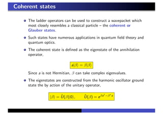
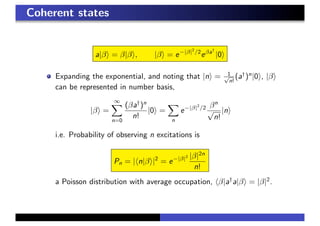
37. Coherent states
|β = ˆU(β)|0 , ˆU(β) = eβa†
−β∗
a
The proof follows from the identity (problem set I),
aˆU(β) = ˆU(β)(a + β)
i.e. ˆU is a translation operator, ˆU†
(β)aˆU(β) = a + β.
By making use of the Baker-Campbell-Hausdorff identity
e
ˆX
e
ˆY
= e
ˆX+ ˆY + 1
2 [ ˆX, ˆY ]
valid if [ˆX, ˆY ] is a c-number, we can show (problem set)
ˆU(β) = eβa†
−β∗
a
= e−|β|2
/2
eβa†
e−β∗
a
i.e., since e−β∗
a
|0 = |0 ,
|β = e−|β|2
/2
eβa†
|0

38. Coherent states
a|β = β|β , |β = e−|β|2
/2
eβa†
|0
Expanding the exponential, and noting that |n = 1√
n!
(a†
)n
|0 , |β
can be represented in number basis,
|β =
∞
n=0
(βa†
)n
n!
|0 =
n
e−|β|2
/2 βn
√
n!
|n
i.e. Probability of observing n excitations is
Pn = | n|β |2
= e−|β|2 |β|2n
n!
a Poisson distribution with average occupation, β|a†
a|β = |β|2
.

39. Coherent states
a|β = β|β , |β = e−|β|2
/2
eβa†
|0
Furthermore, one may show that the coherent state has minimum
uncertainty ∆x ∆p = 2 .
In the real space representation (problem set I),
ψβ(x) = x|β = N exp −
(x − x0)2
4(∆x)2
−
i
p0x
where (∆x)2
= 2mω and
x0 =
2mω
(β∗
+ β) = A cos ϕ
p0 = i
mω
2
(β∗
− β) = mωA sin ϕ
where A = 2
mω and β = |β|eiϕ
.

40. Coherent States: dynamics
a|β = β|β , |β =
n
e−|β|2
/2 βn
√
n!
|n
Using the time-evolution of the stationary states,
|n(t) = e−iEnt/
|n(0) , En = ω(n + 1/2)
it follows that
|β(t) = e−iωt/2
n
e−|β|2
/2 βn
√
n!
e−inωt
|n = e−iωt/2
|e−iωt
β
Therefore, the form of the coherent state wavefunction is preserved
in the time-evolution, while centre of mass and momentum follow
that of the classical oscillator,
x0(t) = A cos(ϕ + ωt), p0(t) = mωA sin(ϕ + ωt)

41. Summary: operator methods
Operator methods provide a powerful formalism in which we may
bypass potentially complex coordinate representations of
wavefunctions.
Operator methods allow us to expose the symmetry content of
quantum systems – providing classification of degenerate
submanifolds and multiplets.
Operator methods can provide insight into dynamical properties of
quantum systems without having to resolve eigenstates.
Quantum harmonic oscillator provides example of
“complementarity” – states of oscillator can be interpreted as a
confined single particle problem or as a system of fictitious
non-interacting quantum particles.