A Calabi-Yau manifold is a smooth space that represents a deformation which smooths out an orbifold singularity. This document discusses superstring theory and fermions in string theories. It introduces the spinning string action and shows that the Neveu-Schwarz model contains a tachyon ground state while the Ramond model contains massless fermions. Combining the two sectors using the Gliozzi-Scherk-Olive projection results in a model with N=1 supersymmetry in ten dimensions.

1. From First Principles January 2017 – R4.7
Maurice R. TREMBLAY
PART X – SUPERSTRING THEORY
A Calabi-Yau manifold is an
example of a smooth space
(i.e., it is Ricci flat – RΜΝ =0)
that represents a deformation
which, from a space-time
point of view, smooths out an
orbifold singularity (i.e., an
infinite amount of curvature
located at each of the points.)
Chapter 2

2. Contents
2017
MRT
PART X – SUPERSTRING THEORY
A History of the Origins of String
Theories
The Classical Bosonic String
The Quantum Bosonic String
The Interacting String
Fermions in String Theories
String Quantum Numbers
Anomalies
The Heterotic String
Compactification and N=1 SUSY
Compactification and Chiral Fermions
Compactification and Symmetry
Breaking
Epilogue: Quantum Gravity
Appendix I: The Gamma Function
Appendix II: The Beta Function
Appendix III: Feynman’s Take on
Gravitation
Appendix IV: Review of Supersymmetry
Appendix V: A Brief Review of Groups
and Forms
References

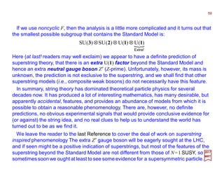
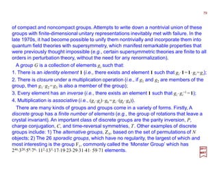
3. If all elementary particles are to be described by strings, it is necessary to introduce
fermionic degrees of freedom. One method of doing this is to invoke the spinning string.
We recall that the Lagrangian S=−[1/(4πα′)]∫dξ 0dξ 1√hhab(∂x/∂ξ a)⋅(∂x/∂ξ b) (c.f., The
Classical Bosonic String chapter) in D dimensions can be interpreted as a set of D
scalar fields xµ(ξ 0,ξ 1) on the two-dimensional world sheet described by ξ 0,ξ 1. To define
the spinning string, we add a similar set of two-dimensional Majorana spinors, λµ(ξ 0,ξ 1),
and use, instead of S=−[1/(4πα′)]∫dξ 0dξ 1 ηab(∂x/∂ξ a)⋅(∂x/∂ξ b) (c.f., The Classical
Bosonic String chapter) the Lagrangian of N=1 SUGRA in two space-time dimensions.
The action can be written as:
3
2017
MRT
∫ ∂−∂∂
′π
−= )(
4
1 2
µ
µ
µ
µ
λρληξ
α
b
a
ba
ab
ixxdS
Fermions in String Theories
where ρ a are two-dimensional Dirac matrices that obey:
abba
ηρρ 2},{ =
with:






−
=
10
01ab
η
A convenient representation of the ρ-matrices is:





 −
=





=
01
10
01
10 10
ρρ and
As usual λ is our last equation for S above denotes λ†ρ 0.
_

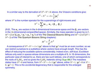
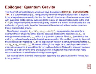
4. (N.B., This action S above has been obtained by starting from the general N=1
SUGRA Lagrangian in two dimensions, which contains a zweibein ea
α and a world-sheet
Majorana spin-3/2 field ψ a. These have been eliminated by using reparametrization
invariance and local SUSY so that we can work in a superconformal gauge in which ea
α =
δ a
α and ψα=0).
4
2017
MRT
By the way, the λµ are spinors on the two dimensional world sheet, but are vectors in
the physical D-dimensional space, so it is not obvious at this stage how, or whether, this
theory can produce fermions (i.e., space-time spinors).
We follow the procedure of the The Classical Bosonic String chapter to obtain the
classical equations of motion. Consider first the open string. For the bosonic variable,
xµ, we obtain the same equations as before, which have the general open string solution
[1/√(2α′)]xµ(τ,σ)=qµ +αm
µτ +iΣn≠0(1/n)αn
µ exp(−inτ)cos(nσ). On the other hand,
minimization of the action with respect to variations in λµ gives the Dirac equation:
0=∂ µ
λρ a
a
as one would expect, provided that we impose the boundary condition (N.B., This
condition ensures that the boundary terms vanish when we integrate by parts):
( )π0010
andatT
== σλδρρλ µ
µ

5. With the representation of ρa given by the matrices ρ0 =[::] and ρ1 =[::] above, if we
write the two-spinor λ as:
5
2017
MRT






=
2
1
λ
λ
λ
the boundary condition λµTρ0ρ1δλµ=0 above becomes:
( )002211 ==⋅−⋅ σλδλλδλ at
This is satisfied if λ1=±λ2 (and δλ1=±δλ2) at each end of the string. The relative sign
between λ1 and λ2 is simply a matter of convention, which we will fix by choosing:
( )021 == σλλ at
But at the other end of the string, σ =π, there are still two distinct choices:
21 λλ =:(R)modelthe Raymond
and
21 λλ −=:(NS)modelthe Schwarz-Neveu

6. Using λ=[λ1 λ2]T above we can write the Dirac equation ρa∂aλµ =0, in component
form:
6
2017
MRT
0)(0)( 21 =∂−∂=∂+∂ λλ στστ and
which have the general solution:
)()( 2211 στλστλ +=−= ff and
where f1 and f2 are arbitrary functions. The requirement λ1 =λ2 (at σ =0) above then
gives:
21 ff =
and the alternative boundary conditions λ1 =λ2 (R) and λ1 =−λ2 (NS) above become:
)()()π2()()()π2( 1111 NSandR ττττ ffff −≡+≡+
It follows that we can write, in analogy to [1/√(2α′)]xµ(τ,σ)=qµ +αm
µτ +iΣn≠0(1/n)αn
µ
⋅exp(−inτ)cos(nσ), &c., for the R model:
∑ 







′= +−
−−
n
ni
ni
nd )(
)(
e
e
),( στ
στ
αστλ
where n are the integers 0,±1,±2,… with dn*=d−n. For the NS model:
∑ 







′= +−
−−
r
ri
ri
rb )(
)(
e
e
),( στ
στ
αστλ
where r are the half-odd-integers ±1/2,±3/2,±5/2,… with br*=b−r.

7. The constraints that arise from the gauge fixing (i.e., ea
α =δ a
α and ψα=0) involve
generalizations of the Virasoro operators Ln
L,R ≡−½Σk=±∞ αk
L,R ⋅αn−k
L,R =0 and Ln
L=Ln
R=0
(for all n) (c.f., The Classical Bosonic String chapter):
7
2017
MRT
0
2
1
2
1
2
1
=⋅





−−⋅−≡ ∑∑ −−
k
kkn
k
knkn ddnkL αα
together with:
0=⋅∑ −
k
kknd α
for the R model, and:
0
2
1
2
1
2
1
=⋅





−−⋅−≡ ∑∑ −−
r
rrn
k
knkn bbnrL αα
0=⋅∑ −
r
kkrb α
together with:
for the NS model.

8. Quantization of the system can now be carried out as in the The Quantum Bosonic
String chapter. The principal difference is that the dn and br obey anticommutation
relations:
8
2017
MRT
0,0, },{},{ srsrmnmn bbdd ++ −=−= δηδη µννµµννµ
and
It turns out that the consistency of the quantization procedure requires:
10=D
for open strings, rather than D=26 needed by the bosonic string.
Again the constraints can be solved most simply in the light-cone gauge, where they
serve to eliminate all but the transverse degrees of freedom.

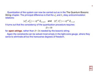
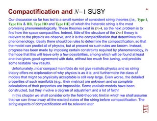
9. In the NS model, we find the mass spectrum:
9
2017
MRT
2
12
−+=′ ∑∑ −−
r
rr
n
nn rM bb ⋅⋅⋅⋅αααα⋅⋅⋅⋅ααααα
The −½ arises from the reordering needed to get the operators into normal order. We
can evaluate this term by following the regularization method of M 2 “=” (1/α′)Σn αααα−n⋅⋅⋅⋅ααααn +
[1/(2α′)]ΣµΣn[αn
µ,α−n
µ ] of the The Quantum Bosonic String chapter et seq.ˆ
ˆ ˆ
We put:
Then we use:








−
−
++=
+=′
∑∑∑∑
∑∑
>>
−−
−−
00
2
2
2
”“
2
1
2
1
”“
rnr
rr
n
nn
r
rr
n
nn
rn
D
r
rM
bb
bb
⋅⋅⋅⋅αααα⋅⋅⋅⋅αααα
⋅⋅⋅⋅αααα⋅⋅⋅⋅ααααα
∑∑∑∑∑
∞
=
−
−
−
−
−−
=
−






−−==−=
1,...2,1,...,,...,,,,...,, 2
1
1
2
1
2
4
2
2
2
4
2
3
2
2
2
1
2
5
2
3
2
1 n
s
s
s
s
ss
r
s
nnrrr
or:
∑∑
∞
=
−=
1,...,,
2
1
2
5
2
3
2
1 n
nr

10. The constant term [(D−2)/2](Σn>0−Σr>0) above is therefore, using ζ(−1)=−1/12 (c.f., The
Quantum Bosonic String chapter):
10
2017
MRT
2
1
12
1
2
3
2
2
12
1
2
3
2
2
”“
2
3
2
2
1
−=⋅⋅
−
−=





−⋅
−
=








⋅
−
∑
∞
=
DD
n
D
n
when D=10 (N.B.,Σnn=1+2+3+…+∞=−1/12=ζ(−1)!)
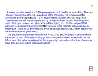
The ground state of the NS spinning string is therefore a tachyon with M2 =−1/(2α′)
from α ′M2 =Σnαααα−n⋅⋅⋅⋅ααααn +Σrrb−r ⋅⋅⋅⋅br −½ above. The first excited state is a massless vector
(i.e., b−½ |0〉), while at M2 =−1/(2α′) we have a vector (i.e., αααα−1 |0〉) and an antisymmetric
tensor (i.e., b−½
µb−½
ν |0〉). (N.B., In this model there are no space-time fermions).

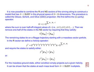
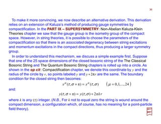
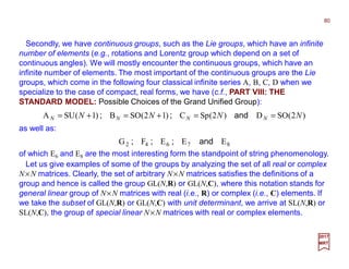
11. In contrast, the R model does have fermions. To see how they arise, note that a
special case of the anticommutation relations {dn
µ,dm
ν}=−ηµνδn+m,0 above is:
11
2017
MRT
µννµ
η−=},{ 00 dd
which implies:
µµ
Γ= id
2
1
0
the Γµ being the Dirac matrices appropriate for the dimension D=10. These operators
only have spinor representations, so the ground state has to be a D=10 Lorentz spinor.
(i.e., we cannot define a unique vacuum state |0〉 satisfying d0 |0〉 =0 because this would
be incompatible with (d0
µ)2=±½ which follows from {d0
µ,d0
ν}=−ηµν above). Other states
are then obtained by acting on this ground-state spinor with dn and αn (n<0). The mass
spectrum is given by:
∑=
−− +=′
,..3,2,1
2
)(
n
nnnn nM dd ⋅⋅⋅⋅αααα⋅⋅⋅⋅ααααα
where the absence of any reordering constant is due to the fact that it cancels between
the αn and dn terms. The ground state |½〉 is therefore a massless fermion. The first
excited space has [mass]2 equal to 1/α′ and is a Rarita-Schwinger spin-3/2 particle (e.g.,
formed by α−1
µ and d−1
µ acting on the ground-state spinor).

12. It is now possible to combine the R and NS sectors of the spinning string to construct a
model that has N=1 SUSY in the physical space of D=10 dimensions. The procedure is
called the Gliozzi, Scherk, and Olive (GSO) projection. We first define the (G-parity)
operator:
12
2017
MRT
1
)1(
−∑ −
−= r rr
G
bb ⋅⋅⋅⋅
where the sum is over half-off-integral values of r (i.e., ±1/2,±3/2,±5/2,…). Then we
remove one-half of the states in the NS sector by requiring that they satisfy:
NSNS φφ =G
The remaining states lie on a Regge trajectory starting with a massless vector particle.
In the R sector we define a helicity operator:
∑ −
−ΓΓΓΓΓΓΓΓΓΓ= r rr dd ⋅⋅⋅⋅
)1)(( 98765432105
γ
and require the states to satisfy either:
RR ψψγ =5
or:
RR ψψγ −=5
For the massless ground state, either condition simply projects out a given helicity.
It can be shown that the states at each mass level form N=1 SUSY multiplets.

13. We now turn to the closed spinning string. Again the bosonic part is like that discussed
in the The Classical Bosonic String chapter and yields [1/√(2α′)]XL
µ = ½qµ +α0
µ (τ +σ )+
½iΣn≠0(1/n)αn
µ L exp[−2in(τ +σ )] and [1/√(2α′)]XR
µ =½qµ +α0
µ (τ −σ )+½iΣn≠0(1/n)αn
µ R
⋅exp[−2in(τ −σ)]. For the fermionic variables we have the general right- or left-moving
solutions given in λ1 = f1(τ −σ ) and λ2 = f2(τ +σ ) above, and we must also impose the
boundary conditions the Raymond model (R): λ1 =λ2 and the Neveu-Schwarz model
(NS): λ1 =−λ2 above, which relate λ(τ ,0) to λ(τ ,π). There are clearly four possibilities
according to whether we impose R or NS type boundary conditions on the right- and left-
moving excitations:
13
2017
MRT
)0,()π,(-
)0,()π,(
)0,()π,(
-
)0,()π,(
)0,()π,(
-
)0,()π,(-
2,12,1
22
11
22
11
2,12,1
τλτλ
τλτλ
τλτλ
τλτλ
τλτλ
τλτλ
−=



=
−=



−=
=
=
NSNS
RNS
NSR
RR

14. In the R-R case, the ground state is a massless boson formed from the tensor product
of two spinors. In the NS-NS case the original SUSY is broken and the ground state is a
tachyon with M2 =−2/α ′, while the first excited state contains a massless spin-2 boson.
The NS-R and R-NS sectors have massless spin-3/2 and spin-1/2 particles as their
ground state and all the excited states are similarly fermionic.
14
2017
MRT
11 55
=−=== LRLR
GG γγand
Again it is possible to define GSO operators and so construct space-time SUSY
models by combining these sectors. The operator G and γ 5 analogous to G=(−1)Σ rb−r⋅⋅⋅⋅br−1
and γ 5 =(Γ0Γ1Γ2Γ3Γ4Γ5Γ6Γ7Γ8Γ9)(−1)Σ rd−r⋅⋅⋅⋅dr above can be defined independently for the R
and L excitations. We thereby obtain three possible types of SUSY string, which are
conventionally called Type IIA, Type IIB, and Type I.
Type IIA (closed String)
Here we use states for which:
This model has N=2 SUSY (i.e., it is supersymmetric in both the L and R sectors). The
massless ground state is an N=2 multiplet containing a graviton of spin 2 and also
particles of spin 3/2, 1, 1/2, and 0. Because of γ 5R =−γ 5L =1 above, both helicities occur,
so the theory is not chiral. At the massless level the theory gives the version of N=2, D=
10 SUGRA that is obtained by a trivial dimensional reduction from N=1, D=11 (i.e., 4 for
space-time plus 7 for a compact manifold) SUGRA discussed in PART IX – SUPER-
SYMMETRY: N=1 SUGRA in Eleven Dimensions.

15. 15
2017
MRT
This model also has N=2 SUSY. The massless ground state is a chiral multiplet
containing the graviton. This N=2, D=10 SUGRA theory cannot be obtained by
dimensional reduction from D=11.
Type IIB (closed string and open string)
Here we have:
11 55
==== LRLR
GG γγand
Type I (closed string and open string)
Here we impose on the Type IIB string the additional condition that the string be
unorientable (i.e., symmetrical under the interchange σ →−σ ). The theory then has only
one supersymmetry and the ground state of the closed string is the chiral graviton
multiplet of the N=1, D=10 SUGRA theory. The open strings form the corresponding
vector multiplet.
I do have to highlight that N=1 SUGRA in ten dimensions removes (e.g., by truncation
of the dimensionally reduced N=1 SUGRA of D=11) the two major difficulties met in N=1
SUGRA in eleven dimensions (i.e., the impossibility of having chiral fermions and the
inadequacy of the gauge group) by the simple prescription of going down from D=11 to
D=10 dimensions! Spinors still have 32 components, so the maximum SUSY, when we
compactify to obtain physical 4-space, is N=8.
Also, the SO(32) Type I superstring is singled out as completely free of anomalies.

16. The graviton multiplet of this theory contains the following fields:
16
2017
MRT
Degrees of freedom .
Symmetric tensor gMN 35
L handed Majorana (vector) spinor ψM 56
Antisymmetric tensor BMN 28
R handed Majorana spinor λ 8
Scalar φ 1
In addition to this multiplet, and in contrast to the D=11 model, it is possible to include
also a Yang-Mills multiplet containing:
Degrees of freedom .
Vector field AM
α 8
L handed Majorana spinor χ α 8
Thus, there are, in principle, two sorts of gauge vector fields in four dimensions: those
that arise from the metric tensor gMN through the Kaluza mechanism, which are
determined by the isometry group of the compact 6-dimensional manifold, and the
fields AM
α from the Yang-Mills multiplet. In applications of this model, the former are
usually ignored (i.e., a compact manifold with no isometries is used), and so Kaluza’s
idea is abandoned completely. Unfortunately, two new problems arise from the arbitrary
nature of the gauge groups. For two particular choices of the gauge group, SO(32)
(Type HO) and E8⊗E8 (Type HE) (N.B., H is for Heterotic – see next chapter) the
anomalies can be made to vanish provided some extra terms are added to the
Lagrangian. What is even more striking is that these extra terms automatically occur
when the model is extracted as the low-energy limit of a superstring theory!

17. Before we can hope to describe the real world by strings, we must find a way of
introducing internal quantum numbers such as charge, color, &c. The physical picture of
a string is of an object that is extended in space, so we have to decide how the charge,
for example, is to be distributed along the string. Clearly, we should do this in a way that
respects the reparametrization invariance, and should avoid any possibility of obtaining
nonquantized charges when strings split (e.g., Figure 2 of the The Interacting String
chapter).
String Quantum Numbers
17
2017
MRT

18. The first satisfactory method, suggested by H. M. Chan and J. E. Paton (1969), had its
beginning in the original manifestation of strings in hadron physics. There, each open
string was assumed to carry a quark (e.g., u, d, or s) at one end and an antiquark (e.g.,
u, d, or s ) at the other. These quarks and antiquarks are regarded as the fundamental 3
and 3 representations of a flavor U(3). Each string then has two U(3) labels and can be
regarded as a meson in the adjoint representation of the group. An external line in a
scattering diagram is therefore associated with one of the 9 (i.e.,=3⊗3=8⊕1) λi
matrices (i=1,2,…,9) of the fundamental representation of SU(3)⊗U(1) (c.f., Table of the
PART VIII – THE STANDARD MODEL: Noether’s Theorem and Global Invariance
chapter where we used the index early Latin index a instead of the above middle Latin
index i). Each scattering amplitude contains a factor:
18
2017
MRT
)(Tr Lkji λλλ
where i, j, k, … label the external particles. If these external particles join different edges
of the world-sheet, several such trace factors are required (e.g., for the diagram in the
Figure we require the factor Tr(λ1λ2)Tr(λ3λ4λ5)).
A diagram in which the trace (Tr) factor has the form Tr(λ1λ2)Tr(λ3λ4λ5).
2
1
3
5
4
−−−−
−−−−
− − −

19. The string diagrams then have continuous quark lines. For example, in the Figure –
Left we see the duality diagram for the single string particle exchange contribution to π+
+K0 →K+ +φ (N.B., π± =ud,du, K0 =ds and K± =us,su are spin-0 mesons while φ is a spin-1
meson) and in the Figure – Right the corresponding diagram for the crossed process K−
+K0 →π− +φ. These duality diagrams picture mesons as qq states bound by stringlike
interactions. Their similarity to the QCD picture explains the (partial) success of such
duality ideas in hadron physics.
19
2017
MRT
Duality diagram for (Left) π+ +K0 →K+ +φ and the crossed process (Right) K− +K0 →π− +φ.
K−K+π+
π−
φK0
s
u
sd
φK0
s
u
ds
−−−−−
−

20. We can also apply this method to introduce internal quantum numbers into
superstrings by imagining that the end of a string is associated with a representation R
of some group and the other end with its conjugate representation R. However, there is a
consistency condition that must be satisfied, because at a pole in a scattering amplitude
(see Figure) the residue must factorize into two, similar, scattering amplitudes. This
condition is only satisfied if R is the fundamental representation of one of the groups
(c.f., Appendix V: A Brief Review of Groups and Forms) U(N), SO(N), or Sp(2N). In the
case of U(N), because R and R are different, the strings are oriented, whereas for SO(N)
or Sp(2N) they are unoriented.
20
Note that in the Chan-Paton method, since quantum numbers are introduced at the
ends of the strings, a closed string can only be a group singlet with no quantum
numbers. This accords with the original identification of the hadronic closed string as a
Pomeron.
2017
MRT
Showing how the residue of a pole in a 3 → 3 amplitude is the product of two 3→ 1 amplitudes.
×
−
−

21. Other methods of introducing quantum numbers onto strings is similar to that used to
introduce spin (and can be regarded as a variant of Kaluza’s idea of associating internal
symmetries with extra space dimensions). For example, we replace the bosonic action
(c.f., the The Classical Bosonic String chapter):
21
by:
2017
MRT
ba
ab xx
ddS
ξξ
ηξξ
α ∂
∂
⋅
∂
∂
′π
−= ∫
10
4
1








∂
∂
∂
∂
+
∂
∂
⋅
∂
∂
′π
= ∫ b
i
a
i
ba
ab xx
ddS
ξ
φ
ξ
φ
ξξ
ηξξ
α
10
4
1
where the φ i are the extra space variables. At this stage the O(N) symmetry associated
with rotations among the φ i in simply an extension of the Lorentz group acting on the xµ.
However, as we shall see in the The Heterotic String chapter, it is possible to treat the φ i
differently and thereby obtain genuine internal symmetries.

22. Typically, in quantized field theories, when a symmetry at the classical level is broken
through quantum corrections these lead to anomalies. Such anomalies can spoil the
renormalizability of the theory, so it may be essential for them to cancel out. If they do,
this puts important restrictions on the theory. On the other hand, the presence of other
types of anomaly is essential to obtain agreement with experiment. Examples include
the decay of the neutral pion and the U(1) problem.
Anomalies
22
The renormalizability of a gauge field theory depends crucially on the cancellation of
the infinities that occur in the various sectors of the theory. This cancellation is a
consequence of relations between Green’s functions that follow from local gauge
invariance. For QED these relations are called the Ward-Takahashi identities, while in
non-Abelian gauge theories they are known as Slavnov-Taylor identities. These
identities are required to prove that the theory is renormalizable. However, there is a
class of diagrams containing closed fermion loops coupled to axial vectors that does not
satisfy such identities. They are variously referred to as the axial vector, of γ 5, or chiral
anomalies. The key result is ∂µJ5µ =2imψ γ5ψ −(e2/8π2)Fµν Fµν (with Fµν =½εµνρσ Fρσ ) for
which the last term is the contribution of the anomaly. For a theory to be renormalizable
these anomalous diagrams must cancel among themselves.
2017
MRT
Because parity is not conserved in weak interactions, a realistic unified theory must
be chiral (i.e., it must treat left- and right-handed fermions differently). With this being
said, we therefore meet the problem of anomalies, and we will try to arrange things
so that they cancel. Amazingly, we will find that for the superstring this is possible for
only two gauge groups: SO(32) and E8⊗E8!
_ ~ ~

23. To see why, we begin by thinking about particle field theories in 10 dimensions. The
analog of (e2/8π2)Fµν Fµν for the anomalous contribution to the divergence of an axial
current J5µ contains the ε symbol with 10 indices:
23
which implies that the simplest diagram producing an anomaly has six external legs (i.e.,
the axial current and the five fields Fµν ).
2017
MRT
10987654321
109876543215
µµµµµµµµµµ
µµµµµµµµµµµ
µ
ε FFFFFJ ∝∂
~
J5λ
Jµ
Jν
γµ
γν
k−p
k+p
p +q
k
γλγ5
q
p
From the usual Feynman rules, the amplitude for this process is:
4444444 34444444 21444444 3444444 21
νµ
µλννλµλµν γγγγγγγγ
JJ
mpkmqkmkmqkmpkmk
kd
T ∫ 





−/+/−/−/−/
+
−/+/−/−/−/
−=
111111
Tr
)π2(
554
4
)3(
The superscript (3) indicates that this is just the third-order contribution.
For example, consider how the axial vector boson couples to two vector bosons. The
lowest-order contribution to this coupling is the triangle diagram with p↔q and µ ↔ν :

24. Thus, instead of the triangle diagrams we now have to consider the hexagon diagram
(see Figure). When we allow for the crossed diagrams (i.e., various orderings of the
vector particles), the group-theoretical factor that occurs in the anomaly is:
24
where Ta are matrices corresponding to the fermion representation of the gauge group,
and the ai label the gauge bosons at each vertex. The complete anomaly is obtained by
summing over all the fermions representations that are included in the theory.
2017
MRT








∑Perm
654321
Tr aaaaaa
TTTTTT
The hexagon coupling of six vector bosons, ai. The internal line is a fermion.
a1 a4
a2 a3
a6 a5

25. As an example, consider the N=1, D=10 SUGRA of the Fermions in String Theories
chapter (c.f., the Type I (closed string and open string) paragraph), which is the low-
energy limit of the Type I superstring. Here the fermions must be in the adjoint represen-
tation of the gauge group, so the freedom to cancel the anomalies does not exist and, in
fact, Tr(ΣPermTa1Ta2…Ta6) above is never zero (for all ai), regardless of the gauge group.
Hence, this version of N=1, D=10 SUGRA (i.e., minimally coupled) is not anomaly-free.
25
For the moment we shall ignore this apparent disaster and turn to the corresponding
calculation of the Type I superstring, which, in spite of its relation to the above particle
theory, gives more promising results. The appropriate hexagon diagram is shown in the
Figure. If we recall the discussion of the String Quantum Numbers chapter, we can
immediately write down the group-theoretical factor as:
2017
MRT
The string diagram analogous to the previous Figure. Again, the internal line is a fermion.
)(Tr)(Tr
Perm
654321
Iaaaaaa




∑ λλλλλλ
where λa are matrices in the fundamental representation of the group. The final factor
Tr(I) is the contribution of the inner loop in the Figure and contributes a factor equal to
the dimension of the fundamental representation.

26. The previous Figure is, however, not the only hexagon diagram in string theory, since
we must also include twisted diagrams. Diagrams with an odd number of twists (see
Figure) are unorientated because there is only one edge, to which all the external
particles are attached (N.B., the internal loop in the Figure – Left is a Möbius strip). The
basic kinematics of these diagrams is the same as for the planar diagram (see previous
Figure), so they all give the same anomaly. The group factors, however, differ in three
ways:
26
2017
MRT
Unorientated diagrams, in which there is only one edge.
We therefore reach the remarkable conclusions that, for SO(32), and only for SO(32),
the anomaly cancels between the planar and the unorientable diagrams.
1. There is no Tr(I) factor, since there is no free edge;
2. There is a factor (±1) due to the interchange (an odd number of times) of the edges of
the strip. In fact, we find −1 for SO(N) groups and +1 for Sp(2N) groups. (N.B., These
diagrams are not possible for U(N) groups because the string in the loop would have RR
rather than RR on its two edges);
3. There is a factor 32 corresponding to the different arrangements of twists (i.e., 6 ways
of having 1 twist or 5 twists, and 20 for 3 twists).
−

27. The final step in the argument is to show that the nonplanar diagrams with 2, 4, or 6
twists (see Figure) are finite and do not contribute to the anomaly. We omit details of this
calculation here, but note that the result is the key to resolving the apparent
contradiction between N=1, D=10 SUGRA and superstrings. To understand why, we
make use of the group-theoretic relation Tr(T6)=(N−32)Tr(λ6)+15Tr(λ4)Tr(λ2) where T6
means any symmetrical product of six matrices in the adjoint representation of SO(N),
and λ6 is the corresponding product of the fundamental representation. If follows that for
SO(32), where the first term cancels, the anomaly from the Tr(T6) relation above is
associated with the second term. This is of course the factor arising from the nonplanar
string diagram (see Figure).
27
2017
MRT
A nonplanar diagram with particles attached to both ends.
The problem, then, is why does field theory have such a term in the anomaly whereas
string theory does not? The answer is that the nonplanar string diagram automatically
includes, in addition to the one-loop field-theory diagrams, tree diagrams in which states
of the closed string are exchanged (c.f., The Interacting String chapter). These diagrams
are themselves anomalous (i.e., they break certain gauge invariances) and cancel the
anomaly in the loops.

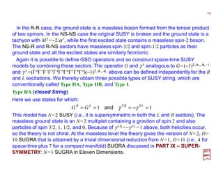
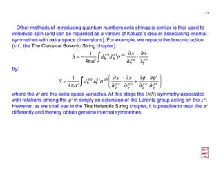
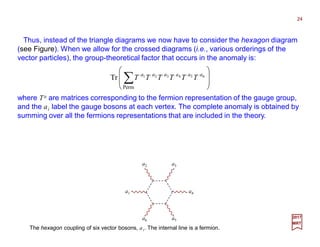
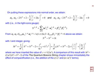
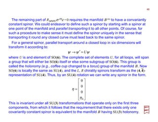
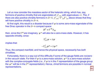
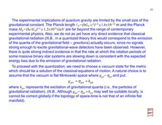
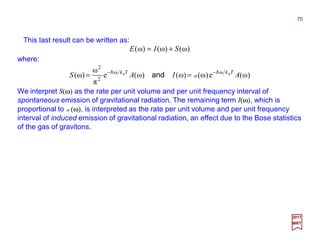
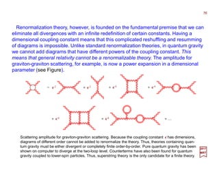
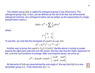
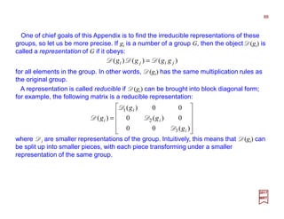
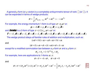
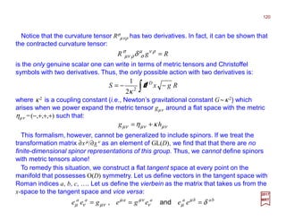
28. The relevant tree diagram involves the exchange of the antisymmetric tensor field BMN
of D=10 SUGRA (c.f., Fermions in String Theories chapter) as in the Figure. The group
factor associated with this diagram clearly factorizes like the last term of the Tr(T6)
relation above. To understand the couplings in the Figure, we first note that BMN appears
in the Lagrangian through a term:
28
where HMNP is the curl of BMN, that is:
2017
MRT
MNP
MNP HH
A coupling of two vector bosons to four vector bosons through the exchange of the antisymmetric tensor
field BMN.
BMN
][ NPMMNP BH ∂=
where […] means that the expression has to be antisymmetrical in the bracketed indices
(e.g., the same way that gauge field appears in the Lagrangian through Fµν =∂µ Aν −∂ν Aµ
≡∂[µ Aν ] as in L =−¼Fµν Fµν−Jµ Aµ of the PART VIII – THE STANDARD MODEL: Field
Equations chapter).

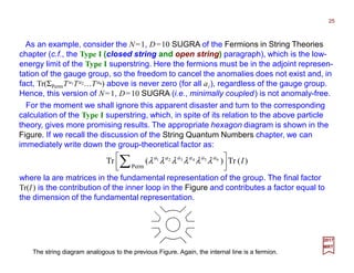
29. In order to maintain a supersymmetry when Yang-Mills multiplets are included, H must
be modified to H′, given by:
29
where ω(Y-M)
MNP is the so-called Yang-Mills Chern-Simon 3-form defined by (c.f.,
Appendix V: A Brief Review of Groups and Forms):
2017
MRT
)M-Y(
ωMNPMNPMNP HH −=′






−= ][][
)M-Y(
3
1
Trω PNMNPMMNP AAAgFA
Here AM and FMN are matrices in the adjoint representation of the gauge group.
It is clear that when we use H′ rather than H in HMNP HMNP above there is a coupling
between BMN and two vector field AM (i.e., the left-hand vertex of the previous Figure).
However, ω(Y-M) is not gauge-invariant, so, in order to maintain the gauge invariance of
the Lagrangian, B must also transform nontrivially under a gauge transformation, a
somewhat surprising conclusion since it appears to be a gauge singlet.
On the other hand, the coupling of B to four gauge bosons, which can occur through a
term:
)(Tr 10987654321
10987654321
MMMMMMMMMM
MMMMMMMMMM
FFFFBε
is only gauge-invariant if B is invariant. It follows that the diagram in the previous Figure
violates gauge invariance, and it is this that allows it to cancel the anomaly!

30. In the original version of N=1, D=10 SUGRA, the coupling ε M1…M10 BM1M2
Tr(FM3M4… M9M10
)
above was not included (because of the requirement of gauge invariance). Remarkably,
however, such a term occurs naturally in the low-energy limit of the superstring, with
exactly the right coefficient to cancel the anomaly if we take the gauge group to be
SO(32)!
30
In addition to the gauge anomalies that we have discussed so far, anomalies also
occur if some of the gauge bosons on the external lines (e.g., the hexagon coupling of
six gauge vector bosons, ai – see first Figure) are replaced by gravitons. Fortunately,
however, these cancel under exactly the same circumstances as the gauge anomalies.
In order to effect this cancellation for N=1, D=10 SUGRA, it is necessary to include also
a gravity 3-form ω(Lor)
MNP in H′MNP above defined in an analogous way to ω(Y-M)
MNP above,
with Aµ replaced by the spin connection ωM
mn, and FMN by the tensor RMN
mn. (N.B., From
PART IX – SUPERSYMMETRY that ωµ
mn plays a similar role to Aµ if we regard general
relativity as a local gauge theory). In fact, the usual conventions require:
2017
MRT
)Lor()M-Y(
ωω −−=′ HH
This additional term does not occur in the simplest form of D=10 SUGRA but it can be
added, and again it occurs automatically in the low-energy limit of the superstring.
In conclusion, the SO(32) Type I superstring is singled out as completely free of
anomalies! By examining its low-energy limit, we learn how the N=1, D=10 SUGRA
theory can also be made anomaly free when SO(32) is the gauge group.

31. Now we find another nice example of the interplay of ideas in theoretical physics. The
argument from superstring theory that we have used to construct the anomaly-free
SO(32) field theory also works for another gauge group, namely E8⊗E8, which has the
same number of generators. Later (c.f., the Compactification of Chiral Fermions chapter)
we shall find that this group is considerably more promising from the point of view of
phenomenology. Unfortunately, however, it is not an allowed group for the type of
superstrings that we considered in the previous String Quantum Numbers chapter and
we are thus led to ask whether there is an alternative way of putting internal quantum
numbers onto strings… Such a method has already been suggested in that chapter and
in the next chapter we shall see how we can employ it to construct the E8⊗E8 string.
31
2017
MRT

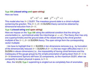
32. The key idea of the heterotic string (meaning hybrid vigor) is to treat right- and left-
moving modes differently. It is a closed string in D=10 for which we take the action to be
(c.f., S=−[1/(4πα′)]∫dξ 0dξ 1ηab(∂x/∂ξ a)⋅(∂x/∂ξ b) of the The Classical Bosonic String and
S=−[1/(4πα′)]∫d2ξ(η ab∂a xµ∂b xµ −iλµρa∂λµ) of the Fermions in String Theories chapters):
32
2017
MRT
∫ 







∂−∂−
∂
∂
∂
∂
′
−= +− A
A
ba
ab xx
ddS λλψψ
ξξ
ηξξ
α
µ
µµ
µ
22
π4
1 10
where ψ µ and λA are Majorana-Weyl fermions on the two-dimensional world-sheet. The
ψ µ are right-moving modes (i.e., functions only of ξ 0 −ξ 1), and the λA (with A=1,2,…,N)
are a set of Lorentz-scalar, left-moving modes (i.e., functions only of ξ 0 +ξ 1). Derivatives
with respect to ξ 0 ±ξ 1 are denoted by ∂±, respectively. From the ψ µ and the right-moving
parts of xµ we construct and N=1 SUSY theory as in the Fermions in String Theories
chapter.
The Heterotic String
_

33. There is, however, no SUSY associated with the left-moving modes. If the λA were
bosonic we would have a (10+N)-dimensional string for which consistency would require
N=16. But in fact, because fermionic modes only contribute half as much to the
cancellation of the conformal anomaly, we require N=32. We separate the λA into two
sets, containing r and 32−r fields, respectively, and impose R or NS conditions. Thus we
have four possibilities: R-R, R-NS, NS-R, and NS-NS, where the first symbol describes
the boundary condition of the first r fields.
33
2017
MRT
where the 8/12 gives the contribution of the ten xµ fields.
1
24
32
2412
8
2
1
)0(-
1
1612
32
2412
8
2
1
)0(-
16
1
24
32
1212
8
2
1
)0(-
1
12
32
1212
8
2
1
)0(-
−=




 −
++−=
+−=




 −
−+−=
+−=




 −
+−−=
=




 −
−−−=
rr
rrr
rrr
rr
α
α
α
α
NSNS
RNS
NSR
RR
The normal ordering constants can be calculated (c.f., as before in the Fermions in
String Theories chapter) and we find:

34. Now, as we noted before in the The Classical Bosonic String chapter, the constraints
require the eigenvalues of the number operators for the right- and left-moving modes to
be equal, so, since summation over the modes give integer values for the former and
either integer or half-odd-integer values for the latter, it follows that the reordering
constant must be integral or half-odd-integral. Hence, we can only allow r=0, 8, or 16.
The r=0 case gives an SO(32) theory of the Type HO already discussed (c.f., Fermions
in String Theories); the r=8 solution does not lead to anything useful; so we take r=16.
34
2017
MRT
Since the ground state of the right-movers has zero mass, the same must be true of
the left-movers. In the NS-NS sector the massless ground state is obtained by operating
with b−½
Ab−½
B |0〉 (i.e., on the vacuum – where b−½
A are creation operators associated
with the λA, &c.) If we take A≤16 and B≥16, or vice versa, these states form the (16,16)
representation of O(16)⊗O(16). On the other hand, with A and B both ≤ or both >16, they
form the (120,1) or (1,120) representations. Of course, at this stage, since we have not
treated the various λA differently, the separation is artificial and in fact the states together
form the adjoint representation of SO(32).
We now include the massless ground states, which are the vacuum states, of the
R-NS and NS-R sectors. By analogy with the discussion of the R sector in the
Fermions in String Theories chapter, these form the spinor representation of the first
or second O(16), respectively. There are in fact two such spinor representations, of
opposite chirality, with dimension 128.

35. It is now possible to define a GSO-type projection (c.f., the Fermions in String Theories
chapter) that removes the (16,16) and one of the chiralities. The remaining states
combine to give the (248,1) and (1,248) adjoint representations of E8⊗E8 (Type HE)
These states are all Lorentz singlets, so, by taking the tensor product with the ground
state of the right movers, we obtain a Yang-Mills, E8⊗E8, N=1 SUSY multiplet! (N.B.,
Although we apparently broke the SO(32) symmetry of the heterotic action S above by
treating A≤16 and A>16 differently, we arrive at a gauge group E8⊗E8, which actually has
the same number of generators).
35
2017
MRT
The graviton multiplet that completes the N=1, D=10 SUGRA theory is obtained from
the tensor product of the right-moving ground state and the lowest xµ excitation for the
left-movers. It is rather surprising that this apparently contrived construction, of which we
have only given an outline here, really works!

36. To make it more convincing, we now describe an alternative derivation. This derivation
relies on an extension of Kaluza’s method of producing gauge symmetries by
compactification. In the PART IX – SUPERSYMMETRY: Non-Abelian Kaluza-Klein
Theories chapter we saw that the gauge group is the isometry group of the compact
space. However, in string theories, it is possible to choose the parameters of the
compactification so that there is an associated degeneracy between string excitations
and momentum excitations in the compact directions, thus producing a larger symmetry
group.
36
2017
MRT
( )24...,,1,0),()π,( ==+ µστστ µµ
xx
and:
rkyy π2),()π,( +=+ στστ
where k is any (±) integer. (N.B., For k not to equal zero the string is wound around the
compact dimension, a configuration which, of course, has no meaning for a point-particle
field theory).
In order to understand this mechanism, we discuss a simple example first. Suppose
that one of the 25 space dimensions of the closed bosonic string of the The Classical
Bosonic String and The Quantum Bosonic String chapters is rolled up into a circle. As
shown in the op cit: Compactification chapter, we denote this coordinate by y and the
radius of the circle by r, so points labeled y and y +2πr are the same. The boundary
condition for the closed string then becomes:

37. We now separate the solution into L- and R-moving parts (c.f., xµ(τ,σ )=XL
µ(τ +σ )+XR
µ
(τ −σ)). For the xµ the general solution is again given by [1/√(2α′)]XL
µ = ½qµ +α0
µ (τ +σ )
+½iΣn≠0(1/n)αn
µ L exp[−2in(τ +σ )] and [1/√(2α′)]XR
µ =½qµ +α0
µ (τ −σ )+½iΣn≠0(1/n)αn
µ R
⋅exp[−2in(τ −σ)]. For the y component, however, we have:
37
2017
MRT
α′
=
2
r
c
with:
)()(),( στστστ −++= RL
YYy
and:
∑ +−
++





++=
′ n
niL
n
L
n
i
kc
c
l
qY )(2
e
1
2
)(2
2
1
2
1
2
1 στ
βστ
α
∑ −−
+−





−+=
′ n
niR
n
R
n
i
kc
c
l
qY )(2
e
1
2
)(2
2
1
2
1
2
1 στ
βστ
α
in which we have introduced the dimensionless constant:

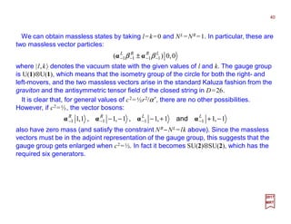
38. Now, with quantization, q and l/c become conjugate variables (c.f., [qµ,α0
ν ]=−igµν):
38
2017
MRT
n
c
lr
π2
2
π2
=
′α
However, q is a periodic variable with period 2πr/√(2α′), so the uniqueness of the wave
function requires that:
iclq −=],[
where n=±integer and hence l has to be a (±) integer too.
The mass of the string as seen in the 25-dimensional space is given by:
00
2 2
αα
α
⋅
′
=M
where of course the scalar product is in 25-dimensions (yikes!). We evaluate this, as in
the The Classical Bosonic String chapter, using the zero-frequency Virasoro constraints
(c.f., Ln
L,R≡−½Σk=±∞ αk
L,R ⋅αn−k
L,R =0 and Ln
L=Ln
R =0, for all n), which here take the form:
02
4
1
0
2
0
00 =−





+−⋅+⋅ ∑∑ ≠
−
≠
−
n
L
n
L
n
n
L
n
L
n kc
c
l
ββαααα
The last two terms in each case are the contributions of the y component.
02
4
1
0
2
0
00 =−





−−⋅+⋅ ∑∑ ≠
−
≠
−
n
R
n
R
n
n
R
n
R
n kc
c
l
ββαααα
and:

39. On putting these expressions into normal order, we obtain:
39
2017
MRT
∑
∞
=
−− +=
1
,,,,,
)(
n
RL
n
RL
n
RL
n
RL
n
RL
N ββαα ⋅⋅⋅⋅
with (i.e., in the light-cone gauge):
02
4
1
2202
4
1
22
2
00
2
00 =





−−+−⋅=





+−+−⋅ kc
c
l
Nkc
c
l
N RL
αααα and
From α0⋅α0 +Σn≠0αααα−n
L, R⋅⋅⋅⋅ααααn
L, R −¼(l/c±2kc)2 −Σn≠0β−n
L, Rβn
L, R =0 above we obtain:
klNN LR
=−
with l and integer, giving:
22
22
2
2
2
)2(
2
4
2
2






′
+





+−+
′
=








++−+
′
=
ααα
rk
r
l
NNck
c
l
NNM RLRL
where we have inserted the value of c=r/√(2α ′). A comparison of this result with M 2 =
(2/α′)(NL +NR −2) of the The Quantum Bosonic String chapter shows immediately the
effect of compactification (i.e., the addition of the (l/r)2 and (kr/α′)2 terms).

40. We can obtain massless states by taking l=k=0 and NL =NR =1. In particular, these are
two massless vector particles:
40
2017
MRT
0,0)( 1111
LRRL
−−−− ± ββ αα
where |l,k〉 denotes the vacuum state with the given values of l and k. The gauge group
is U(1)⊗U(1), which means that the isometry group of the circle for both the right- and
left-movers, and the two massless vectors arise in the standard Kaluza fashion from the
graviton and the antisymmetric tensor field of the closed string in D=26.
It is clear that, for general values of c2=½r2/α′, there are no other possibilities.
However, if c2=½, the vector bosons:
also have zero mass (and satisfy the constraint NR −NL =lk above). Since the massless
vectors must be in the adjoint representation of the gauge group, this suggests that the
gauge group gets enlarged when c2=½. In fact it becomes SU(2)⊗SU(2), which has the
required six generators.
1,11,11,11,1 1111 −++−−− −−−−
LLRR
αααα and,,

41. We shall now show that a generalization of this procedure can be used to give an
alternative description of the heterotic string. As before we take the right-moving modes
to be the D=10 superstring. In contrast to the heterotic action S above we assume that
the left-movers are bosonic and exist in D=26 dimensions,16 of which are compactified.
The general procedure for this compactification is to introduce into the 16-dimensional
Euclidean space a set of 16 vectors eq (q=1,2,…,16), and then to identify points labelled
y and y+√(2α ′)πeq, for and q. We have inserted the factor √(2α′) here so that the eq are
dimensionless (N.B., This is fine-tuning of the model and is necessary to preserve mo-
dular invariance and to obtain the E8⊗E8 symmetry requires for consistencyof the theory).
The closed-string boundary condition (c.f., y(τ,σ +π)=y(τ,σ )+2πkr above) becomes:
41
2017
MRT
∑′+=+
q
qqk eyy π2),()π,( αστστ
where kq are a set of (±) integers.
Since the y are all left-movers (i.e., functions of τ +σ ), the usual expansion (e.g.,
[1/√(2α′)]XL
µ = ½qµ +α0
µ (τ +σ )+½iΣn≠0(1/n)αn
µ L exp[−2in(τ +σ )]) takes the form:
∑ +−
+++=
′ n
ni
n
n
i )(π2
0 e
1
2
)(
2
1
2
1 στ
στ
α
βpyy
Consistency with y(τ,σ +π)=y(τ,σ )+√(2α′)πΣqkqeq above then requires:
that is, p must lie on the lattice defined by the vectors eq.
∑= qqk ep

42. Now, in contrast to the situation where, as in previous examples, we have both L and R
contributions to y, the coefficients of σ and τ in [1/√(2α′)]y= ½y0+p(τ +σ )+½iΣn(1/n)ββββn
⋅exp[−2πin(τ +σ )] above are identical. This means that the quantum condition arising
from periodicity in y is also a condition on p. In fact, single-valuedness of the wave
function requires that exp(2πikq p⋅⋅⋅⋅eq) be equal to unity for all kq, which implies:
42
2017
MRT
the kq being integers and the eq vectors of the so-called dual (or inverse) lattice
satisfying:
∑= qqk ep ~~
~ ~
qqqq ′′ = δee ⋅⋅⋅⋅~
In general a lattice eq and its dual eq do not have any common points, so that p=Σqkqeq
and p=Σqkqeq have no solutions. We consider the case when the two lattices are
identical (i.e., when the lattice is self-dual for this is necessary to preserve modular
invariance, since modular transformations mix the lattice and its dual). This is clearly
sufficient to guarantee the consistency of p=Σqkqeq and p=Σqkqeq; that it is necessary
follows from the requirement of modular invariance of loop amplitudes.
~
~ ~
~ ~

43. In a similar way to the derivation of NR −NL =lk above, the Virasoro conditions give:
43
2017
MRT
2
2
1
1 p+−=− LR
NN
where NR is the number operator for the superstrings of right-movers and:
∑ −− +=
n
nnnn
L
N )( ββαα ⋅⋅⋅⋅⋅⋅⋅⋅
(N.B., The ααααn are vectors in the 8-dimensional transverse space and the ββββn are vectors
in the 16-dimensional compactified space). Similarly, the mass operator is given by (c.f.,
M 2 =(2/α′)Σn(αααα−n
L⋅⋅⋅⋅ααααn
L +αααα−n
R⋅⋅⋅⋅ααααn
R) of the The Classical Bosonic String and M 2 =(2/α′)(NL +
NR −2) of the The Quantum Bosonic String chapters):
R
NM
α′
=
42
A consequence of NR −NL =−1+½|p|2 above is that |p|2 must be an even number, so we
can restrict ourselves to a sublattice where vectors have enough length. This has the
effect of reducing the available options considerably. Indeed even, self-dual, Euclidean
lattices only exist in spaces whose dimensions are a multiple of 8. In 16 dimensions, the
particular case of interest to us, there are two such lattices, one of which corresponds to
the roots of E8⊗E8, and so gives the E8⊗E8 heterotic string (Type HE)! The massless
states have NR =0 and hence, from NR −NL =−1+½|p|2 above, either NL =1, |p|2 =0 or NL =
0, |p|2 =2. This is the accidental degeneracy that is responsible for the enlarged
symmetry.

44. Our discussion so far has led to a small number of consistent string theories (i.e., Type I,
Type IIA & IIB, Type HO and Type HE) of which the heterotic string is the most
promising phenomenologically. These theories exist in D>4, so the next problem is to
find how the space compactifies. Indeed, little of the structure of the D>4 theory is
relevant to the physics we observe, and it is the compactification that determines the
phenomenology. Ideally there should be rules to determine the compactification, so that
the model can predict all of physics, but at present no such rules are known. Instead,
progress has been made by imposing certain constraints required by phenomenology, in
the hope that this will leave only a few possibilities, among which will be found at least
one that gives good agreement with data, without too much fine-tuning, and predicts
some testable new results.
44
2017
MRT
Unfortunately, most compact manifolds do not give realistic physics and so string
theory offers no explanation of why physics is as it is; and furthermore the class of
models that might be physically acceptable is still very large. Even worse, the detailed
properties of such manifolds (e.g., their metrics) are unknown and so complete
calculations of their properties are impossible. Some realistic models have been
constructed, but they involve a degree of adjustment and a lot of faith!
Compactification and N=1 SUSY
In this chapter we shall consider only the field-theoretic limit in which we shall assume
that we can throw away all the excited states of the string before compactification. The
string aspects of compactification will be relevant later.

45. The first requirement that we shall impose on the compactification is that it must give N
=1 SUSY in four dimensions. This is necessary because the mass scale of the theory is
the Planck mass MP and only SUSY seems able to prevent the scalars that are required
by electroweak symmetry breaking from acquiring a mass of this order. On the other
hand, N>1 SUSY is incompatible with the existence of chiral fermions. (N.B., The trivial
compactification onto a 6-torus would leave intact the N=4 SUSY obtained from N=1
SUSY in 10 dimensions).
45
2017
MRT
To obtain N=1 SUSY, the vacuum state must be annihilated by one SUSY generator:
00 =Q
It follows that:
00],[0 =ψQ
and hence that:
000 =δψ
where ψ is any field and δψ is its change under infinitesimal SUSY transformation. We
apply these results to the gravitino ψΜ, for which:
L+= ε
κ
δψ ΜΜ D
1
where ε is an infinitesimal spinorial parameter (c.f., PART IX – SUPERSYMMETRY:
Local Supersymmetry). We assume the omitted terms in δψΜ above involve the field
H′ defined in H′=H−ω(Y-M) −ω(Lor) of the Anomalies chapter and vanish in the vacuum.

46. So, the relation 〈0|δψΜ |0〉=0 above requires the existence of a covariantly constant
spinor ε that satisfies:
46
2017
MRT
This leads to interesting restrictions on the manifold. To find them we note that DΜ ε =0
implies that:
0=εσ ΡΣ
ΜΝΡΣR
0=εΜD
0],[ =εΝΜ DD
Recalling the form of the covariant derivative of a spinor Dµψ =∂µψ −¼iωµ
mnσmnψ (c.f., op
cit: The Inclusion of Matter), and using Rµν
mn =∂µων
mn −∂νωµ
mn +ωµ
m
pων
pn +ων
m
pωµ
pn (c.f.,
op cit: The Einstein Lagrangian), we can write this as:
where RΜΝΡΣ is the Riemann-Christoffel tensor for D=10. We seek a compactification in
which the space takes the form Τ (4)⊗Β (6), where Τ (4) is physical space-time and Β (6) is
the 6-dimensional compact manifold, so RΜΝΡΣ σ ΡΣε =0 above separates into two
equations of similar form.

47. Since we require Τ (4) to be maximally symmetric, we have [c.f., Eq. (13.2.9) of S.
Weinberg, Gravitation and Cosmology, Wiley]:
47
2017
MRT
which can only be satisfied for a nontrivial ε if:
0
6
=εσ ρσ
νσµρ gg
R
)(
12
νρµσνσµρµνρσ gggg
R
R −=
where R is the scalar curvature, so the D=4 part of RΜΝΡΣ σ ΡΣε =0 becomes:
0=R
Thus, the requirement of N=1 SUSY implies a zero cosmological constant, a successful
prediction, but one that is qualified by the presence of other contributions resulting from
the breaking of SUSY, &c., which, unless canceled by fine-tuning, would be many orders
of magnitude too large.

48. The remaining part of RΜΝΡΣ σ ΡΣε =0 requires the manifold Β (6) to have a convariantly
constant spinor. We could endeavor to define such a spinor by starting with a spinor at
one point of the manifold and parallel transporting it to all other points. Of course, for
such a procedure to make sense it must define the spinor uniquely in the sense that
transporting it round any closed curve must lead back to the same spinor.
48
2017
MRT
For a general spinor, parallel transport around a closed loop in six dimensions will
transform it according to:
ψψψ U=′→
where U is and element of SO(6). The complete set of elements U, for all loops, will span
a group that will either be SO(6) itself or else some subgroup of SO(6). This group is
called the holonomy (e.g., coffee cup changed to a torus) group of the manifold Β. Now
SO(6) is locally the same as SU(4), and the L, R chirality spinors transform as the (4,4)-
representation of SU(4). Thus, by an SU(4) rotation we can write any spinor in the form.












=
4
0
0
0
η
η
This is invariant under all SU(3) transformations that operate only on the first three
components, from which it follows that the requirement that there exists only one
covariantly constant spinor is equivalent to the manifold Β having SU(3) holonomy.
−−−−

49. We are thus led to seek compact 6-dimensional manifolds that have metrics with SU(3)
holonomy. These are Calabi-Yau manifolds (a representation of which can be seen on
the cover page of these slides); there are thousands of them in D=6, but none for which
the metric is known. If correction terms going beyond the field-theory limit were included,
then the Calabi-Yau manifolds would not give N=1 SUSY, but it is possible to make
suitable modifications order by order to retain this symmetry.
49
2017
MRT
In summary, therefore, it is possible to obtain N=1 SUSY from the compactification
theory, though there is no particular reason why this should follow from the superstring,
and the requirement itself does not appear to lead to any new predictions.

50. The next requirement is that the compactification should produce some chiral, and
hence massless, fermions in physical space-time. Since all the observed fermions are
chiral (i.e., the two helicity states transform differently under SU(2)), it may be that
chirality is the only reason why nature has any light (i.e.,<<MP) fermions at all. If so,
parity violation is not just some curious accidental feature of nature, but a crucial
requirement if these is to be any nature to think about (or people to do the thinking!) In
string models there are also many nonchiral fermions, as we shall see, but these
presumably have masses that are O(MP).
50
2017
MRT
As noted in PART IX – SUPERSYMMETRY: Kaluza-Klein Models and the Real World,
the chirality operator for D=10 is:
Compactification and Chiral Fermions
32105
)4( ΓΓΓΓ=Γ i
98765432105
)10( ΓΓΓΓΓΓΓΓΓΓ=γ
where the ΓΜ are imaginary 32×32 Dirac matrices in the Majorana representation. We
can also define the analog of the usual D=4 chirality by:
and a similar D=6 chirality operator:
9876545
)6( ΓΓΓΓΓΓ=Γ i
Clearly:
5
)6(
5
)4(
5
)10( ΓΓ=γ
and also:
1)()()( 25
)10(
25
)6(
25
)4( ==Γ=Γ γ

51. Let us now consider the massless sector of the heterotic string, which has, say,
fermions of positive chirality that are eigenstates of γ 5
(10) with eigenvalues +1. The, if
there are also positive chirality fermions in D=4, γ 5
(10)=Γ5
(4)Γ5
(6) above shows that they
will have positive chirality in D=6.
51
2017
MRT
At first sight, this result is a disaster because if ψ is some zero-mass eigenstate of the
free Dirac operator in the D=6 compact space:
Μ
Μ
∂Γ≡/ 6
D
then, since the ΓΜ are imaginary, ψ * will also be a zero-mass state. However, it has
opposite chirality, since:
ψψ ±=Γ5
)6(
implies that:
**5
)6( ψψ ±=Γ−
Thus, the compact manifold, and hence the physical space, necessarily has both
chiralities.
Fortunately, there is a way out of this difficulty if some of the gauge fields are nonzero
in the vacuum state. For then if ψ is a zero-mass solution, ψ * is a zero-mass solution
with the complex-conjugate fields (i.e., if ψ is in the P representation of the gauge group
the ψ * will be in the P* representation). Hence, chiral fermions are possible in nonreal
representations.

52. We must now ask which gauge fields should be nonzero. There are many possibilities,
but a promising way of proceeding is as follows. We have found that to keep N=1 SUSY
it is convenient to put H′=0. Given H′=H−ω(Y-M) −ω(Lor) of the Anomalies chapter, a
natural way to ensure this is to put BMN =0 and to equate the Yang-Mills and gravity 3-
forms:
52
We recall that these 3-forms are traces over vector-field matrices, so a simple way to
satisfy ω(Y-M) =ω(Lor) above is to equate these vector fields. However, the Yang-Mills fields
are matrices in the adjoint representation of the gauge group (i.e.,E8⊗E8), whereas the
spin-connection is in the adjoint representation of SO(6), or, in fact, to preserve N=1
SUSY, in its SU(3) subgroup. Thus, we can only equate the fields in an SU(3) subgroup
of E8⊗E8. The easiest way to do this is to choose the maximal subgroup SU(3)⊗E6 of the
first E8 (say), and to identify the spin connection with the gauge fields in the SU(3) factor.
Thus, the vacuum state of the theory will break E8⊗E8 down to E6⊗E8.
2017
MRT
)Lor()M-Y(
ωω =
This symmetry breaking has the desirable property that the representations of E6, in
contrast to those of E8, are complex, and are therefore suitable for chiral theories. In fact,
the adjoint representation of E8 decomposes under SU(3)⊗E6 according to:
),(),(),(),( 78118273273248 ⊕⊕⊕=
The 27 and 27 are the fundamental representations of E6, and chiral families will occur in
such representations.
−−−−−−−−

53. We can write 27 of E6 in terms of representations of its SO(10) subgroup:
53
2017
MRT
1101627 ⊕⊕=
which, remarkably, contains both the fermion and the standard-model Higgs
representation of the SO(10) of the Grand Unified Theory (c.f., PART VIII – THE
STANDARD MODEL: Possible Choices of the Grand Unified Group chapter). How many
massless representations (i.e., families) there are depends on the Euler characteristic of
the compact manifold (i.e., a topological invariant that happens to be twice the number
of families). In general, the number is large, but examples where it is small do exist.
Finally, note that if we had used the other anomaly-free group, SO(32), in the above
discussion we would not have obtained any complex representations, which is why
E8⊗E8 is preferred!

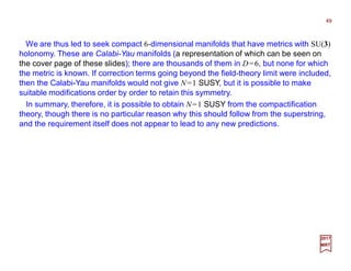
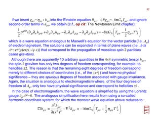
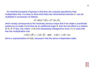
54. In the Compactification and Chiral Fermions chapter we found that the gauge group that
emerges when the gauge fields and spin connection are identified is E6⊗E8. The
massless states of observable physics are singlets of E8 and lie in the 27 of E6, which is
therefore the Grand Unified Theories (GUTs) group. Like for GUT we require E6 to be
broken at a high energy (i.e., at or near the compactification scale, preferably to the
gauge group of the Standard Model – SU(3)⊗SU(2)⊗U(1)). However, the usual Higgs
method of symmetry breaking is not possible here because it requires states of negative
[mass]2, whereas we have taken care to ensure that all masses are zero (or at least real).
54
2017
MRT
Compactification and Symmetry Breaking
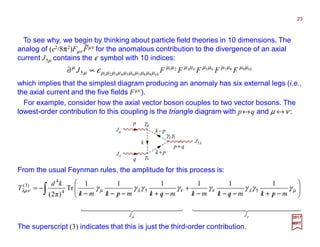
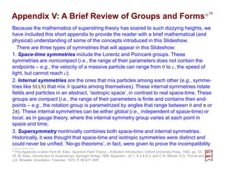
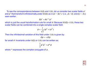
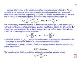
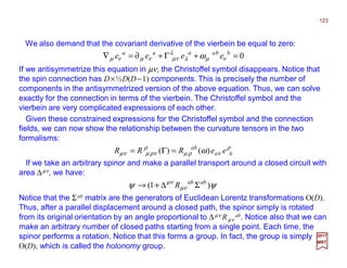
Fortunately, there is an alternative. It relies on the fact that although a zero field-
strength tensor (i.e., Fµν=0) implies that the potential (i.e., Aµ) can be made equal to zero
by a gauge transformation, this can only be achieved globally if the manifold is simply
connected. (N.B., On such a manifold any closed loop can be contracted to a point; thus,
the surface of a sphere is simply connected while the surface of a torus is not – see
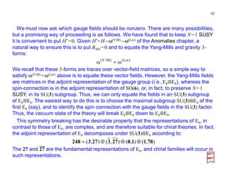
Figure). We shall find that the presence of noncontractible (so-called Wilson) loops
allows a new symmetry-breaking scheme.
Illustrating the differences between a simply and multiply connected manifold. The small loops are drawn
on the surface of the manifolds. The right-hand loop on the torus (Right) cannot be smoothly contracted
to a point.

55. First, we describe how it is possible to construct a nonsimple connected manifold from
a simply connected one Β. Suppose that there is a freely acting discrete symmetry
group F on the manifold. Any element f of F that acts on a point x of the manifold Β will
change it to a new point:
55
2017
MRT
)(xfx →
Here freely acting means that:
xxf ≠)(
for any x on the manifold. In the particular case we are considering, F must be a discrete
group because it can be shown that the 6-dimensional manifold with SU(3) holonomy
cannot have continuous symmetries.
We now alter the topology of Β by identifying the points x and f (x). This does not alter
the local properties of the manifold, in particular the holonomy group. However, even if
the original manifold (i.e., Β) is simply connected, the new one (i.e., Β /F) is not,
because a line from x to f (x) is closed but not contractible to a point.
The possibility of being able to doctor a manifold in this way clearly increases the
number of possible manifolds. It has an immediate advantage, namely, that we can
reduce the number of families, a number which, in simply-connected manifolds, is likely
to be much too large. This is because if x and f (x) are identified then the single-
valuedness requirement:
)]([)( xfx ψψ =
will rule out many solutions.

56. We can now break a symmetry by identifying each element f of F with an element, say
Uf, of the gauge group (i.e., E6), and replacing ψ (x)=ψ [ f (x)] above by:
56
2017
MRT
)]([)( xgfxgf ≡
Using this relation twice, we find:
)()]([ xUxf f ψψ =
)()]}([{)]([)( xUxgfxgUxUU gffgf ψψψψ ===
where fg denotes the mapping:
Hence, from Uf Ugψ =Uf gψ above:
gfgf UUU ≡
which shows that the Uf form a group and hence that F is mapped onto a discrete
subgroup of the gauge group (i.e., E6).
The unbroken subgroup, G, of E6 consists of all the elements V for which ψ (x)=ψ [ f (x)]
above is invariant:
)()]([ xVUxfV f ψψ =
Using ψ (x)=ψ [ f (x)] we can write the left-handed side of this as:
)()]([ xUVxfV f ψψ =
Since these two last equations are true for all ψ, we find:
0],[ =−= VUUVUV fff
So, the unbroken symmetry is the subgroup of E6 that commutes with all the Uf !

57. Two important features of this method of symmetry breaking should now be noted:
First, it is clear that the massless states that survive (i.e., those that satisfy the single-
valuedness requirement, ψ (x)=ψ [ f (x)], above), will lie in particular representations of
the unbroken subgroup G. However, different representations of G will, in general, arise
from different E6 zero modes on Β. Thus, physical fermions, even of one family, will not
necessarily belong to a particular E6 representation. Hence for example, there will be E6
relation between the couplings of the Higgs bosons to the quarks and leptons, which is
good because there is no obvious symmetry in the quark and lepton masses. Second,
there are severe limitations as to the degree of breaking that can be obtained by this
method. The group E6 contains a maximal subgroup SU(3)⊗SU(3)⊗SU(3) and we would
hope to identify one SU(3) with color and break the product of the other two SU(3)s to
SU(2)⊗U(1). But in fact, this is not (quite yet) possible.
57
2017
MRT
One of the successes of the conformal field theory approach is that, with only a few mild
constraints,one finds reasonably acceptable candidates for practical phenomenology.
For example, the heterotic string contains the gauge group E8⊗E8. By making a few
reasonable assumptions about its broken phase, it is possible to break this group down
to E6⊗E8 and finally to E6, which contains the Standard Model’s gauge group,
SU(3)⊗SU(2)⊗U(1). The basic fermion multiplet naturally occurs in the 27 multiplet of E6,
which is consistent with known grand unified theory (GUT) phenomenology. Thus, it is
surprising that, with very few minimal assumptions, we are naturally led to the following
symmetry breaking scheme:
)(U)(SU)(SUEEEEE 68688 123 ⊗⊗→→⊗→⊗

58. Now, suppose,first, that F is a cyclic group consisting of one element f, which satisfies:
58
2017
MRT
1=N
f
Then, from Uf Ug =Uf g above:
1)( =N
fU
Now if Uf is to commute with SU(3)⊗SU(2)⊗U(1), it can be written parametrically as:










⊗










⊗










=
−
ε
δ
γ
β
β
β
α
α
α
00
00
00
00
00
00
00
00
00
1
fU
with α3 =γδε =1 because SU(N) matrices have unit determinant. In order to satisfy (Uf)N =
1 above we also require:
1===== NNNNN
εδγβα
The unbroken symmetry consists of all matrices that commute with Uf =[MMM]⊗[MMM]⊗[MMM]
above:










−
⊗⊗










−⊗⊗⊗










−
⊗
200
010
001
000
010
001
200
010
001
IIIIII and,
)(U)(U)(U)(SU)(SU 11123 ⊗⊗⊗⊗
where the generators of the three U(1) factors may respectively be taken to be:

59. If we use noncyclic F, then the analysis is a little more complicated and it turns out that
the smallest possible subgroup that contains the Standard Model is:
59
2017
MRT
Here (at last! readers may well exclaim) we appear to have a definite prediction of
superstring theory, that there is an extra U(1) factor beyond the Standard Model and
hence an extra neutral gauge boson Z′ (Z-prime). Unfortunately, however, its mass is
unknown, the prediction is not exclusive to the superstring, and we shall find that other
superstring models (i.e., composite weak bosons) do not necessarily have this feature.
{
Extra!
)(U)(U)(SU)(SU 1123 ⊗⊗⊗
In summary, string theory has dominated theoretical particle physics for several
decades now. It has produced a lot of interesting mathematics, has many desirable, but
apparently accidental, features, and provides an abundance of models from which it is
possible to obtain a reasonable phenomenology. There are, however, no definite
predictions, no obvious experimental signals that would provide conclusive evidence for
(or against) the string idea, and no real clues to help us to understand the world has
turned out to be as we find it.
We leave the reader to the last Reference to cover the deal of work on superstring
inspired phenomenology The extra Z′ gauge boson will be eagerly sought at the LHC,
and if seen might be a positive indication of superstrings, but most of the features of the
superstring beyond the Standard Model are not different from those of N=1 SUSY, so
sometimes soon we ought at least to see some evidence for a supersymmetric particle.

60. The theory of general relativity, which we have discussed in PART IX – SUPERSYMME-
TRY, is a purely classical (i.e., nonquantum) theory of the gravitational field. It appears
to be adequate experimentally, but the fact that all other forces of nature are associated
with quantized fields strongly suggests that it is only an approximation (valid in the limit
h→0) to the proper quantum theory of gravity. Indeed, it is almost inconceivable that the
unification of gravity with the other forces could be achieved without such a quantum
theory that includes gravity.
60
2017
MRT
The Einstein equation Rµν −½Rgµν +Λgµν =−8πGNTµν demonstrates the need for a
quantum theory of gravity rather directly, because it relates the Ricci tensor, Rµν , to
energy-momentum tensor, Tµν, which is a quantum operator. Thus Rµν (and hence the
metric gµν ) should surely also be treated as an operator. We could of course try to avoid
this conclusion by replacing Tµν by its expectation value in a particular quantum state Rµν
−½Rgµν +Λgµν =−8πGN〈Tµν〉. However, although this might be a useful approximation in
many circumstances, it would lead to very odd predictions if taken too seriously such as
allowing us to observe the time of wavefunction reduction (if this phenomenon really
occurs) and even to send faster-than-light messages!
We instead follow the more likely road of assuming that gravity, like other forces, has
to be quantized.
Epilogue: Quantum Gravity

61. The experimental implications of quantum gravity are limited by the small size of the
gravitational constant. The Planck length lP =(hGN /c3)1/2 ≅1.6×10−35 m and the Planck
mass MP =(hc/GN)1/2 ≅ 1.2×1019 GeV are far beyond the range of contemporary
experimental physics. Also, we do not as yet have any direct evidence that classical
gravitational radiation (N.B., in a quantized theory this would correspond to the emission
of the quanta of the gravitational field – gravitons) actually occurs, since no signals
strong enough to excite gravitational-wave detectors have been observed. However,
there is quite strong indirect evidence in that the rate at which the rotation periods of
some massive binary star systems are slowing down is consistent with the expected
energy loss due to the emission of gravitational radiation.
61
2017
MRT
To proceed with the quantization, we need to choose a vacuum state for the metric
which should be a solution of the classical equations of motion. A natural choice is to
assume that the vacuum is flat Minkowski space where gµν=ηµν and put:
µνµνµν η hg +=
where hµν represents the excitation of gravitational quanta (i.e., the particles of
gravitational radiation). (N.B., Although gµν =ηµν +hµν may well be suitable locally, is
cannot be correct globally if the topology of space-time is not that of an infinite flat
manifold).

62. If we insert gµν=ηµν +hµν into the Einstein equation Rµν −½Rgµν=−8πGNTµν, and ignore
second-order terms in hµν, we obtain (c.f., op cit: The Newtonian Limit chapter):
62
2017
MRT
which is a wave equation analogous to Maxwell’s equation for the vector particle (i.e.,Aµ)
of electromagnetism. The solutions can be expanded in terms of plane waves (i.e., à la
Aµ=ε µ(q)exp(−iq⋅x)) that correspond to the propagation of massless spin-2 particles
called gravitons.






−−=∂∂−∂∂−∂∂+∂∂ λ
λνµνµσνρµµρσννµσρσρνµ
σρ
ηη TTGhhhh N
2
1
π8)(
2
1
Although there are apparently 10 arbitrary quantities in the 4×4 symmetric tensor hµν ,
the spin-2 graviton has only two degrees of freedom corresponding, for example, to
helicities ±2. The reason is that the remaining eight degrees of freedom correspond
merely to different choices of coordinates (i.e., of the {xµ}) and have no physical
significance – they are spurious degrees of freedom associated with gauge invariance.
Again, the situation is analogous to electromagnetism where, of the four degrees of
freedom of Aµ, only two have physical significance and correspond to helicities ±1.
In the case of electromagnetism, the wave equation is simplified by using the Lorentz
gauge ∂µ Aµ=0. The analogous simplification here results from using a so-called
harmonic coordinate system, for which the monster wave equation above reduces to:






−−=∇−
∂
∂
≡ λ
λνµνµνµ
νµ
νµ η TTGh
x
h
h N
2
1
π16
)(
2
20
2

63. Several important differences from electromagnetism should now be noted:
63
2017
MRT
First, the higher-order terms, neglected in this last equation, give rise to interactions
between three and more gravitons. Thus, like gluons but unlike photons, gravitons
interact with each other!
Second, we note that canonical quantization involves writing causal commutation rules
such that commutators between field operators (e.g., hµν (x), hµν (x)) are zero when x and
x are spacelike-separated (i.e., when c2∆t2 <∆r2 and s2 > 0). However, the concept of a
spacelike interval is only defined with respect to some metric and since our metric is
itself an operator, we have a major difficulty. It is usual to define the commutators of the
theory with respect to the background metric ηµν , but then it is not obvious that strict
causality is maintained.
This third difference is that, unlike the fine structure constant of QED for the
electromagnetic coupling, α =e2/hc, which is dimensionless, the corresponding quantity
in gravity (i.e., GN /hc) has dimension [mass]−2. Thus the index of divergence of the
interaction (i.e., δi ≡bi+(3/2) fi +di −4, where bi is the number of bosons, fi is the number
of fermions, and di is the number of derivatives) is equal to +2, which has the serious
consequence that, at least according to simple power-counting arguments, the theory is
not renomalizable!

64. The combination of quantum theory with special relativity has always caused
difficulties. By demanding that the theories of the other forces must be renormalizable
we have been led to schemes that seem to accord with the observed world. However,
when we move from special to general relativity the power-counting argument suggests
that this solution is no longer available. The only remaining hope for obtaining a sensible
quantum gravity theory is apparently to look for a truly finite theory (i.e., one in which all
the divergences cancel). This is not the case with pure gravity based on the monster
wave equation above, which if we play with it for a while reduces to:
64
2017
MRT
(where we put ηµν =diag(+1,−1,−1,−1)) and it seems likely to be possible only if there is a
conspiracy between the diagrams associated with all the various types of interactions.
Presumably this can only happen if gravity is unified with the other forces of nature.
Indeed, the requirement of finiteness might lead to a unique form for such a unification.






−−=
∂∂
∂
+
∂∂
∂
−
∂∂
∂
+
∂∂
∂
−+
∂∂
∂
−
∂∂
∂
∑∑∑ ===
λ
λνµνµ
µ
ν
µ
ν
ν
µ
ν
µ
νµνµνµ
η TTG
xx
h
xx
h
xx
h
xx
h
h
xx
h
xx
h
N
i
i
i
i
i
i
i
ii
2
1
π16
3
1
2
0
0
23
1
2
0
0
23
1
2
00
2
It is worth noting that even if the complete theory of everything, including gravity, is
finite, the requirement that the low-energy effective theory (not including gravity)
should be renormalizable! If it were not true there would be no reason why the low-
energy calculations should give the right answer…

65. At present there does not exist any complete and self-consistent quantum theory of
gravitation.* Were such a theory to exist, and at its simplest level, we would interpret a
gravitational plane wave, with wave vector kµ and helicity ±2, as consisting of gravitons;
quanta with energy-momentum vector pµ =hkµ and spin component in the direction of
motion ±2h (N.B., h=1.054 ×10−27 erg sec is Dirac’s constant). Since kµ kµ =0, the graviton
is a particle of zero mass, like the photon. According to energy-momentum tensor:
)]([)]([
)(
)( 33
t
E
pp
t
td
txd
pxT xxxx −−−−−−−− δδ
νµν
µνµ
==
* These next 11 slides are taken in part from S. Weinberg, Gravitation and Cosmology, Wiley (1973), pp. 285-289.
2017
MRT
since x0(t)=t and pµ =Edxν/dt, an assembly of gravitons, all of which have four-momenta
pµ =hkµ, is:
N
ω
νµ
νµ
kk
T h=
where N is the number of gravitons per unit volume. Comparing this with the result for a
gravitational plane wave (i.e., 〈tµν 〉=(1/16πGN)kµ kν (|ε+|2 +|ε−|2)) we then conclude that the
number density of gravitons with helicity ±2 in a plane wave is N± =(ω/16πhGN)|ε±|2 (N.B.,
GN =6.6732 ×10−8 dyn cm2 g−2 is Newton’s gravitation constant). The total number density
is:






−=+= −+
2
*
2
1
)(
16π
ω σ
σνµ
νµ
εεε
NGh
NNN
65

66. The power emitted as gravitational radiation by an arbitrary system as giving the rate
dΓ of emitting gravitons of energy hω into the solid angle dΩ:






−Ω==Γ
2*
)ω,(
2
1
)ω,()ω,(
π
ω
ω
1
kTkTkTd
G
Pdd N σ
σ
νµνµ
hh
2017
MRT
However, the energy-momentum tensor Tµν (k,ω) must now be interpreted as a matrix
element of an energy-momentum tensor operator between final and initial states. In
particular, in the quadrupole approximation the total rate for an atom to make a transition
a→b by emitting gravitational radiation is:






→−→→=→Γ
2*
5
)(
3
1
)()(
5
ω2
)( baDbaDbaD
G
ba jijiji
N
h
where:
∫≡→ )()()( *3
e xxx ajibji xxdmbaD ψψ
with ψa and ψb the initial and final state wave functions. For instance, the rate for decay
of the 3d (ml =2) state of the Hydrogen atom into the 1s state with emission of one
graviton is (N.B., the transition occurs because a graviton is emitted with ω=(Ea −Eb)/h):
1
sec−−
×==→Γ 44
26157
3
e
23
105.2
)137(53
2
)s1d3(
h
cmGN
Needless to say, there is no chance of observing such a transition!
66

67. We can also consider a process that is going on anyway, such as a collision between
particles, and ask what is the probability of a graviton being emitted during the process.
∑ 





−⋅
⋅⋅
=
Ω MN
MNMN
MN
MNN
mmPP
kPkP
G
dd
Ed
,
222
2
2
2
1
)(
))((π2
ω
ω
ηη
2017
MRT
where the sums over N and M run over all particles in the initial (η =−1) or final (η =+1)
states, and divide by hω. The probability of emitting a graviton in the solid angle dΩ and
in a frequency range dω is then:
∑ 





−⋅
⋅⋅
Ω=
MN
MNMN
MN
MN
c
N
mmPP
kPkP
ddP
G
Pd
,
222
2
2
2
1
)(
))((
ω
ωπ2
ω ηη
h
where Pc is the probability of the collision occurring without graviton emission.
The gravitational energy per solid angle and per frequency interval emitted at
frequency ω and direction k is now given by:ˆ
67

68. It should be noted that the emission probability dP is proportional to dω/ω (N.B., the
factor P⋅k in the denominator being proportional to ω), so the total probability for
emission of gravitational radiation in a collision diverges logarithmically both at ω→∞
and ω→0!
2017
MRT
The first, or ‘ultraviolet’, divergence at ω=∞ was encountered classically, and arises
just because of our approximation that the collision occurs instantaneously, it is to be
eliminated by cutting off the ω-integral at ω~1/∆t ~E/h, where ∆t is the duration of the
collision and, via the uncertainty principle, E is some typical energy characteristic of the
collision.
The second, or ‘infrared’, divergence at ω=0 is a purely quantum mechanical problem;
it enters here only because we divided the emitted energy dE by hω to get the emission
probability, It is removed by recognizing that Pc, the probability for the collision to occur
without gravitational radiation, is itself logarithmically divergent because of emission and
reabsorption of virtual gravitons, and that the divergences cancel.
−
We see that once we have accepted the most elementary ideas about the quantum
nature of gravitational radiation, we are inevitably let to the full infrastructure of real and
virtual gravitons.
68

69. The quantum interpretation of gravitational radiation allows a simple derivation of the
relations between absorption and emission of gravitons. Imagine a blackbody cavity in a
body of temperature T that is so large and dense that it is opaque to gravitational
radiation. The cavity will be filled with both electromagnetic and gravitational radiation in
equilibrium with the container. By using the same statistical arguments that give the
Planck distribution law for electromagnetic radiation (c.f., PART II – MODERN
PHYSICS: Planck’s Resolution of the Problem), we may conclude that the number of
gravitons (i.e., N ) per unit volume, n, with frequency between ω and ω+dω is:
1e
1
ω
π
ω
ω)ω( ω2
2
−
= TkB
dd h
n
2017
MRT
where kB =1.38×10−16 erg K−1 is Boltzmann’s constant. In order for equilibrium to be
maintained, it is necessary that the absorption rate A(ω) of a single graviton in the
container wall be related to the rate per unit volume E(ω)dω of graviton emission
between frequencies ω and ω+dω by:
ω)ω(ω)ω()ω( dEdA =n
69

70. This last result can be written as:
2017
MRT
where:
)ω()ω()ω( SIE +=
)ω(e)ω()ω()ω(e
π
ω
)ω( ωω
2
2
AIAS TkTk BB hh −−
== nand
We interpret S(ω) as the rate per unit volume and per unit frequency interval of
spontaneous emission of gravitational radiation. The remaining term I(ω), which is
proportional to n(ω), is interpreted as the rate per unit volume and per unit frequency
interval of induced emission of gravitational radiation, an effect due to the Bose statistics
of the gas of gravitons.
70

71. Since S(ω) and I(ω) above remain valid even if the gravitational radiation is not in
equilibrium with matter, so that n(ω) is not given by n(ω)dω=(ω2/π2)dω[exp(hω/kBT)−1]−1
above. It is only necessary that the matter be in thermal equilibrium at temperature T.
For instance, we can calculate the rate S(ω) of spontaneous emission of gravitons per
unit volume and per unit frequency interval in a nonrelativistic gas of particles of number
density na (e.g., of type a particles, &c.):
∑ ∫ Ω
Ω=
),(
252
sin
π5
8
ω ba
ab
abbaab
N
d
d
dvnn
G
d
dP
θ
σ
µ
2017
MRT
This ω−3 behavior can make A(ω) surprisingly large for low-frequency gravitons in
gases at high temperature. However, the effect of induced emission is to reduce the
effective absorption rate by a factor hω/kBT. There does not appear to be any situation
in the present universe where the absorption of gravitational radiation plays any
important role!
∑ ∫ Ω
Ω=
),(
252
3
sin
ω5
π8
)ω(
ba
ab
abbaab
N
d
d
dv
G
A θ
σ
µ nn
h
and dividing it by hω, provided that the graviton frequency ω is in the range ωc <<ω<<kBT/h,
where ωc is the collision frequency, µ is the reduced mass, v is the relative velocity, and θ is
the scattering angle in the barycentric frame. Applying S(ω)=(ω2/π2)exp(−hω/kBT)A(ω)
above then gives the absorption rate of such gravitons as:
71

72. The preceding remarks describe what may be called a semiclassical theory of
gravitation. The development of a true quantum theory of gravitation is unfortunately
much more difficult.
∑ −
+=
r
xkir
r
xkir
r aadxh ]e)()(e)()([)( *)(†)(3 σ
σ
σ
σ
νµνµνµ εε kkkkk
2017
MRT
One approach is to construct an interaction Hamiltonian that can create and destroy
gravitons, and then calculate transition probabilities as a power series in this interaction.
Usually the Hamiltonian would be built up out of quantum fields, of the form:
where εµν =ε (r)
µν (k) is a polarization tensor for a graviton of momentum hk and helicity r,
and ar(k) and ar
†(k) are the corresponding annihilation and creation operators, characte-
rized by the transformation relation:
srsr aa δδ )(])(),([ 3†
kkkk ′=′ −−−−
The difficulty in this approach comes from the fact that the operator hµν above cannot be
a Lorentz tensor as long as the helicity sum is limited to the physical values r=±2 (i.e., a
true tensor would have helicities 0 and ±1 as well as ±2). It is true that we can start with
a true tensor and then subject εµν to a gauge transformation that will eliminate the
unphysical helicities 0 and ±1, but once we choose a gauge in this way, hµν is no
longer a tensor.
and
0])(),([])(),([ ††
=′=′ kkkk srsr aaaa
72

73. To put this another way, a gauge condition, such as the statement that ε13, ε23, ε10, ε20,
ε00, ε03, and ε33 vanish for k in the 3-direction, is not Lorentz invariant, so if we define
these components to vanish, then under a Lorentz transformation Λµ
ν , hµν will not simply
transform into Λµ
ρ Λν
σ hρσ , but will be subjected to an additional gauge transformation:**
µ
ν
ν
µ
ρσ
σ
ν
ρ
µνµ
ξξ
xx
hh
∂
∂
+
∂
∂
+ΛΛ→
2017
MRT
It is no easy task to construct a Hamiltonian out of such an object in such a way as to
obtain Lorentz invariant transition probabilities.
** S. Weinberg, “Photons and Gravitons in Perturbation Theory: Derivation of Maxwell’s and Einstein’s Equations”, Phys. Rev.,
138, B988 (1965).
73

74. There are two possible ways out of this difficulty…
2017
MRT
One possibility is to accept the nonlinear character of hµν , and use the noncovariant
Hamiltonian formalism to derive Lorentz-invariant rules for the calculation of transition
amplitudes which essentially leads to Loop Quantum Gravity.† This works fairly easily in
electrodynamics, but the self-interaction of the gravitational field has so far prevented
the completion of this program in general relativity.
† See “Covariant Loop Quantum Gravity: An Elementary Introduction to Quantum Gravity and Spinfoam Theory”, C. Rovelli
and F. Vidotto, Cambridge University Press (2014).
A different method, pioneered by R. P. Feynman (c.f., Appendix III: Feynman’s Take on
Gravitation and the Article), is to start out with manifestly Lorentz-invariant calculational
rules, and then tinker with them to prevent the appearance of unphysical particles with
helicities 0 and ±1 in physical states. This program has been successfully carried out to
completion in the work of L.D. Fadeev and V.N. Popov, Phys. Lett., 25B, 29 (1967); S.
Mandelstam, Phys. Rev., 175, 1604 (1968); and B.S. DeWitt, Phys. Rev., 162, 1195,
1239 (1967) with erratum, Phys. Rev., 174, 1834 (1968).
74

75. 75
Naïve attempts to quantize Einstein’s theory of gravitation have met with disappointing
failure. One of the first to point out that general relativity would be incompatible with
quantum mechanics was Heisenberg, who noticed that the presence of a dimensional
coupling constant would ruin the usual renormalization program.
If we set h≡h/2π=1 and c ≡1 there still remains a dimensional constant even in the
Newtonian theory of gravity, F=GN m1m2/r2, the gravitational constant GN which has
dimensions of centimetres squared. When we power expand the metric tensor gµν
around that space with the (flat) metric ηµν being the matrix diag(−,+,+,+), we introduce
the coupling constant κ, which has dimensions of centimeters in CGS units:
νµνµνµ κη hg +=
Therefore:
2
~ κNG
In this system of units, where the only unit is the centimeter, this coupling constant κ
becomes the Planck length, 10−33 cm or 1019 GeV, which is far beyond the reach of
experimentation!
2017
MRT

76. 76
Renormalization theory, however, is founded on the fundamental premise that we can
eliminate all divergences with an infinite redefinition of certain constants. Having a
dimensional coupling constant means that this complicated reshuffling and resumming
of diagrams is impossible. Unlike standard renormalization theories, in quantum gravity
we cannot add diagrams that have different powers of the coupling constant. This
means that general relativity cannot be a renormalizable theory. The amplitude for
graviton-graviton scattering, for example, is now a power expansion in a dimensional
parameter (see Figure).
Scattering amplitude for graviton-graviton scattering. Because the coupling constant κ has dimensions,
diagrams of different order cannot be added to renormalize the theory. Thus, theories containing quan-
tum gravity must be either divergent or completely finite order-by-order. Pure quantum gravity has been
shown on computer to diverge at the two-loop level. Counterterms have also been found for quantum
gravity coupled to lower-spin particles. Thus, superstring theory is the only candidate for a finite theory.
2017
MRT
κ 2= κ 2+ κ 4+ κ 4+
κ 6+ κ 6+ + …

77. Unfortunately, the formulation of general rules for the calculation of transition
probabilities in the quantum theory of gravitation has only confirmed the presence of
another difficulty: The theory contains infinities, arising from integrals over large virtual
momenta. Quantum electrodynamics contains similar infinities, but only in three or four
special places, where they can be dealt with by a renormalization of mass, charge, and
wave function (c.f., PART VII – QUANTUM ELECTRODYNAMICS: Overview of
Renormalization in QED). In contrast, the quantum theory of gravitation contains an
infinite variety of infinities, as can be seen by an elementary dimensional argument: The
gravitational constant has dimensions h/m2, so a term in a dimensionless probability
amplitude of order GN
n
will diverge like a momentum-space integral ∫ p2n−1dp. In this
respect, the theory of gravitation is more like other nonrenormalizable theories, such as
the Fermi theory of beta decay, than it is like quantum electrodynamics.
2017
MRT
Despite these difficulties, there is one very important conclusion that can already be
drawn from the quantum theory of gravitation: It is quite impossible to construct a
Lorentz invariant quantum theory of particles of mass zero and helicity ±2 without
building some sort of gauge invariance into the theory, because only in this way can the
interaction of the nontensor field hµν generate Lorentz-invariant transition amplitudes.
It therefore appears that the Principle of Equivalence, on which the whole of classical
general relativity is based, is itself a consequence of the requirement that the quantum
theory of gravitation should be Lorentz invariant.
77

78. Because the mathematics of superstring theory has soared to such dizzying heights, we
have included this short appendix to provide the reader with a brief mathematical (and
physical) understanding of some of the concepts introduced in this Slideshow.
78
2017
MRT
Appendix V: A Brief Review of Groups and Forms*
* This Appendix is taken from M. Kaku, Quantum Field Theory – A Modern Introduction, Oxford University Press, 1993, pp. 33-
45, M. Kaku, Introduction to Superstrings, Springer-Verlag, 1988, Appendix - §A.1, A.2 & A.3, and C.W. Misner, K.S. Thorne and
J.A. Wheeler, Gravitation, Freeman, 1973, P. 69 & P. 90ff.
There are three types of symmetries that will appear in this Slideshow:
1. Space-time symmetries include the Lorentz and Poincaré groups. These
symmetries are noncompact (i.e., the range of their parameters does not contain the
endpoints – e.g., the velocity of a massive particle can range from 0 to c, the speed of
light, but cannot reach c);
2. Internal symmetries are the ones that mix particles among each other (e.g., symme-
tries like SU(N) that mix N quarks among themselves). These internal symmetries rotate
fields and particles in an abstract, ‘isotropic space’, in contrast to real space-time. These
groups are compact (i.e., the range of their parameters is finite and contains their end-
points – e.g., the rotation group is parametrized by angles that range between 0 and π or
2π). These internal symmetries can be either global (i.e., independent of space-time) or
local, as in gauge theory, where the internal symmetry group varies at each point in
space and time;
3. Supersymmetry nontrivially combines both space-time and internal symmetries.
Historically, it was thought that space-time and isotropic symmetries were distinct and
could never be unified. ‘No-go theorems’, in fact, were given to prove the incompatibility

79. of compact and noncompact groups. Attempts to write down a nontrivial union of these
groups with finite-dimensional unitary representations inevitably met with failure. In the
late 1970s, it had become possible to unify them nontrivially and incorporate them into
quantum field theories with supersymmetry, which manifest remarkable properties that
were previously thought impossible (e.g., certain supersymmetric theories are finite to all
orders in perturbation theory, without the need for any renormalization).
79
2017
MRT
There are many kinds of groups and groups come in a variety of forms. Firstly, A
discrete group has a finite number of elements (e.g., the group of rotations that leave a
crystal invariant). An important class of discrete groups are the parity inversion, P,
charge conjugation, C, and time-reversal symmetries, T. Other examples of discrete
groups include: 1) The alternative groups, ZN, based on the set of permutations of N
objects; 2) The 26 sporadic groups, which have no regularity, the largest of which and
most interesting is the group F1, commonly called the ‘Monster Group’ which has
246⋅320⋅59⋅76⋅ 112⋅133⋅17⋅19⋅23⋅29⋅31⋅41⋅ 59⋅71 elements.
A group G is a collection of elements gi such that:
1. There is an identity element 1 (i.e., there exists and element 1 such that gi ⋅1=1⋅gi =gi);
2. There is closure under a multiplication operation (i.e., if g1 and g2 are members of the
group, then g1 ⋅g2 =g3 is also a member of the group);
3. Every element has an inverse (i.e., there exists an element 1 such that gi ⋅gi
−1 =1);
4. Multiplication is associative (i.e., (gi ⋅gj)⋅gk =gi ⋅(gj ⋅gk)).

80. Secondly, we have continuous groups, such as the Lie groups, which have an infinite
number of elements (e.g., rotations and Lorentz group which depend on a set of
continuous angles). We will mostly encounter the continuous groups, which have an
infinite number of elements. The most important of the continuous groups are the Lie
groups, which come in the following four classical infinite series A, B, C, D when we
specialize to the case of compact, real forms, we have (c.f., PART VIII: THE
STANDARD MODEL: Possible Choices of the Grand Unified Group):
80
2017
MRT
Let us give examples of some of the groups by analyzing the set of all real or complex
N×N matrices. Clearly, the set of arbitrary N×N matrices satisfies the definitions of a
group and hence is called the group GL(N,R) or GL(N,C), where this notation stands for
general linear group of N×N matrices with real (i.e., R) or complex (i.e., C) elements. If
we take the subset of GL(N,R) or GL(N,C) with unit determinant, we arrive at SL(N,R) or
SL(N,C), the group of special linear N×N matrices with real or complex elements.
of which E6 and E8 are the most interesting form the standpoint of string phenomenology.
)2(SOD)2(SpC)12(SOB)1(SUA NNNN NNNN ==+=+= and;;
87642 EEEFG and;;;
as well as:

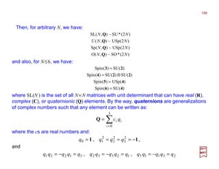
81. To illustrate some of these abstract concepts, it will prove useful to take the simplest
possible nontrivial example, O(2), or rotations in two dimensions. Even the simplest
example is surprisingly rich in content. Our goal is to construct the irreducible
representations of O(2), but first we have to make a few definitions.
81
2017
MRT
invariant22
=+ yx
If we rotate the plane through an angle θ, then the coordinates [x,y] of the same point
in the new system are given by:












−
=





y
x
y
x
θθ
θθ
cossin
sincos
We will abbreviate this by (N.B., sum over repeated indices):
jjii
xx O=
where x1 =x and x2 =y. (N.B., For the rotation group, it makes no difference whether we
place the index i as a superscript, as in xi, or as a subscript, as in xi).
We know that if we draw a straight line on a piece of 8½×11 paper, then rotate this
sheet of paper, the length of the straight line drawn on the paper will remain constant. If
[x,y] describe the coordinates of a point on a plane, then this means that, by the
Pythagorean theorem, the following length is an invariant under a rotation about the
origin:*
* Recall that we expressed this earlier as (N.B., in the following slides you can associate the invariant in component form too):
invariant=ii xx

82. For small angles θ, the matrix equation [:]=[::][:] above can be reduced to:
82
2017
MRT
yyyxxx δδ −=+= and
where:
xyyx θδθδ −== and
since cosθ →1 and sinθ →θ as θ →0, or simply:
jjii
xx εθδ =
where ε ij is antisymmetric and ε 12 =−ε 21 =1. These matrices form a group; for example,
we can write down the inverse of any rotation, given by O−1(θ) = O(−θ):






==−
10
01
)(O)(O 1θθ
We can also prove associativity, since matrix multiplication is associative.

83. The fact that these matrices preserve the invariant length places restrictions on them.
To find the nature of these restrictions, let us make a rotation on the invariant distance:
83
2017
MRT
that is, this is invariant if the Oij matrix is orthogonal:
jjkkijijkkijjiii
xxxxxxxx === ]OO[OO



≠
=
==
kj
kjkjkiji
if
if
0
1
OO δ
where δ is called the Kronecker delta, or, more symbolically:
11 =OOT
To take the inverse of an orthogonal matrix, we simply take its transpose. The unit matrix
1 is called the metric of the group.

84. The rotation group O(2) is called the orthogonal group in two dimensions. The
orthogonal group O(2), in fact, can be defined as the set of all real, two-dimensional
orthogonal matrices. Any orthogonal matrix can be written as the exponential of a single
antisymmetric matrixτ:
84
2017
MRT
N
N
N
)(
!
1
e)(O
0
τθθ τθ
∑
∞
=
≡=
where:






−
=
01
10
τ
To see this, we note that the transpose of exp(θτ ) is exp(−θτ):
1
Oe)e(O −−
=== τθτθ TT
Another way to prove the exp(θτ )=ΣN(1/N!)(θτ )N identity above is simply to power
expand the right-hand side and sum the series. We then see that the Taylor expansion of
the cosθ and sinθ functions re-emerge. After summing the series, we arrive at:






−
=+=
θθ
θθ
θτθτθ
cossin
sincos
sincose 1
All elements of O(2) are parametrized by one angle θ. We say that O(2) is a one-
parameter group (i.e., it has dimension dim=1).

85. Let us now take the determinant of both sides of the following equation:
85
2017
MRT
1)]O([det)O(detO)(det)OO(det 2
=== TT
This means that the determinant of O is equal to ±1. If we take detO=1, then the
resulting subgroup is called SO(2), or the special orthogonal matrices in two dimensions.
The rotations that we have been studying up to now are members of SO(2).






−
=
10
01
P
This last transformation corresponds to a parity transformation:
yyxx −→→ and
A parity transformation P takes a plane and maps it into its mirror image, and hence it is
a discrete, not continuous transformation, such that P2 =1.
However, there is also the curious subset when detO=−1. This subset consists of
elements of SO(2) time the matrix:

86. An important property of groups is that they are uniquely specified by their
multiplication law. It is easy to show that these two dimensional matrices Oij can be
multiplied in succession as follows:
86
2017
MRT
)(O)(O)(O θθθθ += kikjji
which simply corresponds to the intuitively obvious notion that if we rotate a coordinate
system by an angle θ and then by an additional angle θ, then the net effect is a rotation
of θ +θ. In fact, any matrix D(θ) (not necessarily orthogonal or even 2×2 in size) that
has this multiplication rule:
)π2()()()()( +=+= θθθθθθ DDDDD and
forms a representation of O(2), because it has the same multiplication table.
−
−

87. For our purposes, we are primarily interested in the transformation properties of fields.
For example, we can calculate how a field φ(x) transforms under rotations. Let us
introduce the operator:
87
2017
MRT








∂
∂
−
∂
∂
=
∂
∂
≡ 1
2
2
1
x
x
x
xi
x
xiL j
iji
ε
Let us also define:
Li
U θ
θ e)( =
Then we define a scalar field as one that transforms under SO(2) as:
scalar)()()()( 1
==−
xUxU φθφθ
(N.B., To prove this equation, we use the fact that exp(A)Bexp(−A)= B+[ A,B]+
(1/2!)[ A,[A,B]]+(1/3!)[ A,[A,[A,B]]]+…) with the commutator [A,B]=AB−BA, then we
reassemble these terms via a Taylor expansion to prove the transformation law).
We can also define a vector field φ i(x), where the additional i index also transforms
under rotations:
vector)()(O)()()( 1
=−=−
xUxU jjii
φθθφθ
This result can be generalized to include an arbitrary field φ a(x) that transforms under
some representation of SO(2) labeled by some index a. Then the field transforms as:
)()()()()( 1
xUxU bbaa
φθθφθ −=−
D
where Dab is some representation, either reducible or irreducible, of the group.

88. One of chief goals of this Appendix is to find the irreducible representations of these
groups, so let us be more precise. If gi is a number of a group G, then the object D(gi) is
called a representation of G if it obeys:
88
2017
MRT
)()()( jiji gggg DDD =
for all elements in the group. In other words, D(gi) has the same multiplication rules as
the original group.
A representation is called reducible if D(gi) can be brought into block diagonal form;
for example, the following matrix is a reducible representation:










=
)(00
0)(0
00)(
)(
3
2
1
i
i
i
i
g
g
g
g
D
D
D
D
where Di are smaller representations of the group. Intuitively, this means that D(gi) can
be split up into smaller pieces, with each piece transforming under a smaller
representation of the same group.

89. The principle goal of our approach is to find all irreducible representations of the group
in question. This is because the basic fields of physics transform as irreducible
representations of the Lorentz and Poincaré groups. The complete set of finite-
dimensional representations of the orthogonal group comes in two classes, the tensors
and spinors. We will now discuss the tensors, and will discuss the spinors shortly.
89
2017
MRT
)()](O)(O[)( jijjiiji
BABA θθ=
One simple way of generating higher representations of O(2) is simply to multiply
several vectors together. The product AiB j, for example, transforms as follows:
This matrix Oii(θ)Oj j(θ) forms a representation of SO(2). It has the same multiplication
rule as O(2), but the space upon which it acts is 2×2 dimensional. We call any object that
transforms like the product of several vectors a tensor.
In general, a tensor T i jk… under O(2) is nothing but an object that transforms like the
product of a series of ordinary vectors:
tensorOO
,,,,,, 21221121
==
LL
L
jjjijiii
TT
The transformation of T i jk… is identical to the transformation of the product x ix jx k….
This product forms a representation of O(2) because the following matrix:
has the same multiplication rule as SO(2).
)(O)(O)(O)(O
,,,,,,;,,, 22112121
θθθθ NNNN jijijijjjiii
L
LL
≡
- -

90. The tensors that we can generate by taking products of vectors are, in general,
reducible (i.e., within the collection of elements that compose the tensor, we can find
subsets that by themselves form representations of the group). By taking appropriate
symmetric and antisymmetric combinations of the indices, we can extract irreducible
representations.
90
2017
MRT
uuUu iθ
θ e)( ==
We can also show the equivalence between O(2) and yet another formulation. We can
take a complex object u=a+ib, and say that it transforms as follows:
The matrix U(θ) is called a unitary matrix, because:
1=†
UU
The set of all one-dimensional unitary matrices U(θ)=exp(iθ) defines a group called
U(1). Obviously, if we make two such transformations, we find:
)(
eeee θθθθθθ ++
== iiiii
We have the same multiplication law as O(2), even though this construction is based on
a new space, the space of complex one-dimensional numbers. We thus say that:
)(~)(SO 12 U
θτθ i
ee =
This means that there is a correspondence (i.e., ~) between the two, even though they
are defined in two different spaces (N.B., recall the earlier result exp(θτ)=1cosθ +τ sinθ):

91. To see the correspondence between O(2) and U(1), let us consider two scalar fields φ 1
and φ 2 that transform infinitesimallyunder SO(2) as inδx i =θε ijx j (i.e.,δx=θ y andδy=−θ y)
seen earlier:
91
2017
MRT
jjii
φεθφδ =
which is just the usual transformation rule for small θ. Because SO(2)~U(1), these two
scalar fields can be combined into a single complex scalar field:
)(
2
1 21
φφφ i+=
Then the infinitesimal variation of this field under U(1) is given by:
φθφδ i−=
for small θ. Invariants under O(2) or U(1) can be written as:
φφφφ *
2
1
=ii
where * expresses the complex conjugate of φ .

92. The previous group O(2) was surprisingly rich in its representations. It was also easy to
analyze because all its elements commuted with each other. We call such a group an
Abelian group. Now, we will study non-Abelian groups, where the elements do not
necessarily commute with each other. We define O(3) as the group that leaves distances
in three dimensions invariant:
92
2017
MRT
invariant222
=++ zyx
where x i =Oij x j. Generalizing the previous steps for SO(2), we know that the set of 3×3,
real, and orthogonal matrices O(3) leaves this quantity invariant. The condition of
orthogonality reduces the number of independent numbers down to 32 −6=3 elements.
Any member of O(3) can be written as the exponential of an antisymmetric matrix:
∑ =
=
3
1
eO i i
i
i τθ
whereτ i has purely imaginary elements.There are only three independent antisymmetric
3×3 matrices, so we have the correct counting of independent degrees of freedom.
Therefore O(3) is a three-parameter Lie group, parametrized by three angles (e.g., the
Euler angleα,β,γ ).
−

93. These three antisymmetric matrices τ i can be explicitly written as:
93
2017
MRT










−−==









 −
−==










−
−==
000
001
010
001
000
100
010
100
000
321
iii zyx
ττττττ and,
By inspection, this set of matrices can be succinctly represented by the fully
antisymmetric ε ijk tensor as:
kjikji
iετ −=][
where ε 123 =+1. These antisymmetric matrices, in turn, obey the following properties:
kkjiji
i τεττ −=],[
This is an example of a Lie algebra (not to be confused with the Lie group). The
constants ε ijk appearing in the algebra are called the structure constants of the algebra.
A complete determination of the structure constants of any algebra specifies the Lie
algebra, and also the group itself.

94. For small angles θ i, we can write the transformation law as:
94
2017
MRT
jkkjii
xx θεδ =
As before (i.e., Lk=iε ijk xi ∂ j earlier) we will introduce the operators:
kjkjii
xiL ∂≡ ε
We can show that the commutation relations of Li satisfy those of SO(3). Let us construct
the operator:
ii
Lii
U θ
θ e)( =
Then a scalar and a vector field, as before, transform as follows:
)()(]O[)()()()()(O)()()( 111
xUxUxUxU jjiijjii
φθθφθφθθφθ −−−
=−= or
As in the case of O(2), we can also find a relationship between O(3) and a unitary group.
Consider the set of all unitary, 2×2 matrices with unit determinant. These matrices form a
group, called SU(2), which is called the special unitary group in two dimensions. This
matrix has 8−4−1=3 independent elements in it. Any unitary matrix, in turn, can be
written as the exponential of a Hermitian matrix H, where H=H*T =H†:
Hi
U e=
Again, to prove this relation, simply take the Hermitian conjugate of both sides:
1†
ee
†
−−−
=== UU HiHi

95. Since an element of SU(2) can be parametrized by three numbers, the most
convenient set is to use the Hermitian Pauli spin matrices. Any element of SU(2) can be
written as:
95
2017
MRT
2
e
ii
i
U σθ
=
where:






−
==




 −
==





==
10
01
0
0
01
10 321 zyx
i
i
σσσσσσ and,
where σ i satisfy the relationship:
22
,
2
k
kji
ji
i
σ
ε
σσ
=








We now have exactly the same algebra as SO(3) as in [τ i,τ j]=iε ijkτ k above. Therefore,
we can say:
)(SU~)(SO 23

96. To make the correspondence more precise, we will expand the exponential and then
recollect terms, giving us:
96
2017
MRT
2
ee
iiii
ii θσθτ
↔
where θ i =niθ and (ni)2 =1. The correspondence is then given by:






+





=
2
sin)(
2
cose )2( θ
σ
θθσ kki
ni
ii
where the left-hand side is a real, 3×3 orthogonal matrix. Even though these two
elements exist in different spaces, they have the same multiplication law. This means
that there should also be a direct way in which vectors [x,y,z] can be represented in
terms of these spinors. To see the precise relationship, let us define:






+
−
=•=
zyix
yixz
h xσx)(
Then the SU(2) transformation:
1−
= UhUh
is equivalent to the SO(3) transformation:
xOx •=

97. Now let us take a subgroup of GL(N,R), the orthogonal group O(N), which consists of
all possible N×N real matrices that are orthogonal:
97
2017
MRT
∑
−
=
=
)1(½
1
eO
NN
i i
i
λθ
The real numbersθ i are called the parameters of the group, and there are thus ½N(N−1)
parameters in O(N) (e.g., N=3, we get 3). The number of parameters of a lie group is
called its dimension.The commutatorof two of these generators yields another generator:
k
k
jiji f λλλ =],[
where the f s are called the structure constants of the algebra(N.B.,sum over repeated
k as usual). Notice that the structure constants determine the algebra completely.
This obviously satisfies all four of the conditions for a group. Any orthogonal matrix can
be written as the exponential of an antisymmetric matrix:
1=T
OO
It is easy to see that:
A
eO=
In general, an exponential matrix has ½N(N−1) independent elements. Thus we can
always choose a set of ½N(N−1) linearly independent matrices, called the generators λi,
such that we can write any element of O as:
1
OeeO −−
=== AAT
T

98. Notice that if we take cyclic combinations of three commutators, we get an exact
identity:
98
2017
MRT
0]],[,[0]],[,[]],[,[]],[,[ ][ ==++ kjijikikjkji λλλλλλλλλλλλ or
By expanding out these commutators, we find that the combinations identically cancels
to zero. This is called the Jacobi identity and must be satisfied for the group to close
properly. By expanding out the Jacobi identity, we now have a constraint among the
commutators that must be satisfied, or else the group does not close:
00 ][ ==++ m
lk
l
ji
m
lj
l
ik
m
li
l
kj
m
lk
l
ji ffffffff or
Of course, the set of orthogonal matrices closes under multiplication(i.e.,O(θ 1)O(θ 2) =
O(θ 3)). A more complicated problem is to prove that this particular parametrization of the
orthogonalgroup,withgeneratorsandparameters,closesundermultiplication.Let us write:
CBA
eee =
Fortunately, the Baker-Campbell-Hausdorff theorem shows that C equals A plus B plus
all possible multiple commutators of the A and B (i.e., the Baker-Campbell-Hausdorff
formula is exp(A)exp(B)=exp(A +B+½[ A,B]+…)). But since the A and B satisfy the Jacobi
identities,the set of all possible multiple commutators of A and B only creates linear
combinations of the generators. Thus, the group closes under multiplication.
Notice that the structure constants of the algebra form a representation, called the
adjoint representation. If we write the structure constants as a matrix f k
ij =[λk]ij.Thus,
the structure constants themselves form a representation.

99. We can always choose the commutation relations to be:
99
2017
MRT
dacbcadbcbdadbcadcba
MMMMMM δδδδ ++−=],[
for the antisymmetric matrix Mab. One convenient representation of the algebra is now
given by:
a
j
b
i
b
j
a
iji
ba
M δδδδ −~][
which, we can show, satisfies the commutation relations of the group.
Let us define a set of N elements xi that transforms as a vector under the group O(N):
jjii xx O=
In general, we can also define a tensor Tµ1,µ2,µ3,…,µp
of rank p that transforms in the same
way as the product of p ordinary vectors xµi
:
pppp
TT µµµµµνµνµνµννννν ,...,,,,,,,,...,,, 321332211321
OOOO L=

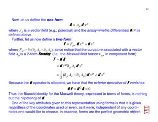
100. In addition to the vector representation of O(N), we have the spinor representation of
the group. Let us define the Clifford algebra:
100
2017
MRT
baba
δ2},{ =ΓΓ
Now define a representation of the generators in terms of these Clifford numbers:
],[
4
1 baba
i
M ΓΓ=
The Clifford numbers themselves transforms as vectors:
)(],[ acbbcacba
iM Γ−Γ=Γ δδ
In general, these Clifford numbers can be represented by 2N×2N matrices [Γa]µν for the
group O(2N). Therefore, a spinor ψµ that transforms under O(2N) has 2N elements and
transforms as:
ννµ
ζ
µ ψψ ]e[
baba
M
=
where the Ms are written in terms of the Clifford algebra and the ζ variables are
parameters.

101. For the group O(2N+1), we need one more element. This missing element is Γ2N+1 =
Γ1Γ2…Γ2N. We can easily check that this new element allows us to construct all the M
matrices for O(2N+1).
101
2017
MRT
invariant=ii xx
Let us now try to construct invariants under the group. Orthogonal transformations
preserve the scalar product:
If xi =Oij xj, then:
iiii xxxxxx == OOT
This invariant can be written:
jjii xx δ
where the metric is δij. In principle, we could have a metric with alternating positive and
negative signs along the diagonal,ηij, which would create elements in ηij, then the set of
matrices that preserve this form is called O(N, M ):
lilkkjji ηη =O]O[ T
where ε (i)=±1. If all the elements of ε are positive, this gives a generalization of the
group O(N). If the signs alternate, then the group is noncompact. Special cases
include: 1) Projective group, O(2,1); 2) Lorentz group, O(3,1); 3) de Sitter Group,
O(4,1); 4) anti-de Sitter group, O(3,2); 5) Conformal group, O(4,2).
and
jiji i δεη )(=

102. For example, the de Sitter group can be constructed by taking the generators of O(4,1)
and then writing the fifth component as Pa ~ M5a, then the algebra becomes:
102
2017
MRT





++−=
−=
=
dacbcadbcbdadbcadcba
cbabcacba
baba
MMMMMM
PPMP
MPP
ηηηη
ηη
],[
],[
],[
:)1,(O 4
Notice that this is almost the algebra of the Poincaré group. In fact, if we make the
substitution:
aa
PrP ±→
then the only commutator that changes is:
baba
M
r
PP 2
1
],[ =
where r is called the de Sitter radius. This means that if we go around a circle in de
Sitter space and return to the same spot, we will be rotated by a Lorentz transforma-
tion from our original orientation. Notice that if r goes to infinity, we have the Poincaré
group. Thus, r corresponds to the radius of a five-dimensional universe such that, if r
goes to infinity, it becomes indistinguishable from the flat four-dimensional space of
Poincaré. Letting the radius go to infinity is called the Wigner-Inönü contraction and
will be used extensively in supergravity theories. After the contraction, the de Sitter
group becomes the Poincaré group.

103. The group SU(N), which stands for special unitary N×N matrices with complex
coefficients, consists of all possible N×N complex matrices that have unit determinant
and are unitary:
103
2017
MRT
1=†
UU
Any unitary matrix can be written as the exponential of a Hermitian matrix, H† =H, that is:
H
U e=
We can show that U† =exp(−iH†)=exp(−iH)=U−1.
Let N elements in a complex vector ui transform linearly under SU(N):
jjii uUu =
The N complex vectors ui generate the fundamental representation of the group.
invariant*
=ii uu
iikkjjiiii uuuUUuuu *†**
][ ==
If ui =Uij uj, it is easy to check that:
The metric tensor for the scalar product is again δij. If we were to reserve some of
the signs in this diagonal matrix, the groups that would preserve this metric are called
SU(N,M ). An example of this would be the conformal group SU(2,2).
−

104. Any N×N complex traceless Hermitian matrix has N2−1 independent elements and
hence can be written in terms of N2−1 linearly independent matrices λi. Thus, any
element of SU(N) can be written as:
∑
−
=
=
12
1
e
N
i i
i
i
U
λρ
The Baker-Hausdorff theorem then guarantees that the group closes under this
parametrization and that we can write the algebra of the group as:
k
k
jiji fi λλλ =],[
again, knowledge of the structure constants f k
ij determines the algebra completely.
We can also construct representations of SU(N) out of spinors. If we have the group
O(2N ), then SU(N) is a subgroup. If we construct the elements:
)(
2
1 212 jjj
iA Γ−Γ= −
where Γ2j are Grassman variables, then the generators of SU(N) can be written as:
∑=
kj
k
kj
aja
AA
,
†
][λλ
2017
MRT
Thus, we have an explicit representation for the inclusion:
)2(O)(SU NN ⊂
104

105. The symplectic groups Sp(2N ) are defined as the set of 2N×2N real matrices S that
preserve an antisymmetric metric η:
2017
MRT
lilkkjji ηη =S]S[ T
where:
jjii uu S=
and
















−
−
=
OMMMM
L
L
L
L
0100
1000
0001
0010
jiη
105

106. Fortunately, there is a series of accidents that allow us to make local isomorphisms
between groups. For example, O(2) is locally isomorphic to U(1):
2017
MRT
)()(O 12 U=
To see this, we simply note the correspondence between a matrix element of O(2) and
U(1):
θτθ
θθ
θθ i
e
cossin
sincos
e ↔





−
=
Thus, they have the multiplication law θ1 +θ2 =θ3.
Another accident is:
)(SU)(O 23 =
The easiest way to prove this is to note that the Pauli spin matrices σi are 2×2 complex
matrices with the same commutation relations as the algebra of O(3). Thus:
∑∑ ==
↔
3
1
3
1
ee i i
i
i i
i
i σθτθ
where the matrix on the left is a 3×3 orthogonal matrix and the one of the right is a
unitary matrix.
106

107. Another useful accident is:
2017
MRT
)(SU)(SU)(O 224 ⊗=
To prove this, we note that the generators Mij of O(4) can be divided into two sets:
and
},,{ 323121 MMMA =
},,{ 434142 MMMB =
Notice that the A and B matrices separately generate the algebra of O(3) and that:
0],[ =BA
Thus, we can parametrize any element of O(4) such that it splits up into a product of O(3)
and another commutating O(3). Thus, we have proved that an element of O(4) can be
split up into the product of two elements of a commutating set of SU(2) groups.
107

108. Unfortunately, these three prior accidents are the exception, rather than the rule, for
Lie groups. We list some of the accidents (N.B., the symbol ‘ ~ ’ means ‘corresponds to’):
2017
MRT
dim = 3:
),(SL~),(Sp~);1,(SO~);1,(SU
),(SL~),(~)(USp~),(SO~),(SU
R2R2R2C1
Q1Q12R3C2 U
dim = 6:
),(SL),(SL~);2,(SO
),(SL~);1,(SO
),(SL),(SU~)(*SO
),SU(),SU(~),(SO
R2R2R2
C2R3
R2C24
C2C2R4
⊗
⊗
⊗
dim = 10:
),(Sp~);2,(SO
)2,(USp~);1,(SO
)(USp~),(SO
R4R3
2R4
4R5
dim = 15:
);(SU~);3,(SO
);2,(SU~);2,(SO
);1,(SU~)(*SO
),(SL~)(*SU~);1,(SO
),(SU~),(SO
R4R3
C2R4
C36
Q24R5
C4R6
108

109. Then, for arbitrary N, we have:
2017
MRT
)2(*SO~),(O
)2(USp~),(Sp
)2(USp~),(
)2(*SU~),(SL
NN
NN
NNU
NN
Q
Q
Q
Q
)(SU)(Spin
)(USp)(Spin
)(SU)(SU)(Spin
)(SU)(Spin
46
45
224
23
=
=
⊗=
=
and also, for N≤6, we have:
where SL(N ) is the set of all N×N matrices with unit determinant that can have real (R),
complex (C), or quaternionic (Q) elements. By the way, quaternions are generalizations
of complex numbers such that any element can be written as:
∑=
=
3
0i
ii qcQ
where the cs are real numbers and:
,, 11 −==== 2
3
2
2
2
10 qqqq
and
231131233231221 qqqqqqqqqqqqqqq =−==−==−= ,,
109

110. Now, it is often convenient to describe a gauge theory (e.g., Yang-Mills theory) in the
mathematical language of forms (i.e., especially when working in higher dimensions D).
As a concrete example, we will begin by making an association with Maxwell’s theory
first, then provide a generalization to exterior calculus. Next we will review how spinors
enter into coordinate covariance and Lorentz transformations such as to pave the way
for an overview of forms as they apply in Yang-Mills theories where local gauge
invariance is important.
110
2017
MRT
Let us define the derivative operator as:
0},{ ==∧+∧∧−=∧ νµµννµµννµ
xxxxxxxxxx dddddddddd or
µ
µ
∂= xdd
Notice that because the derivatives ∂µ ≡∂/∂xµ commute (as opposed to… anticommute):
0],[ =∂∂=∂∂−∂∂ νµµννµ
we therefore obtain:
02
== ddd
which makes dddd nilpotent, by definition.
0=∧ µµ
xx dd
and
So, to start with, let the infinitesimal differentials dddd xµ be antisymmetric under an
operation ∧ that we call the wedge product; that is, the anticommutator:

111. Now, let us define the one-form:
111
2017
MRT
µ
µ xA dA =
where Aµ is a vector field (e.g., potential) and the antisymmetric differentials d xµ as
defined above.
Further, let us now define a two-form:
νµ
νµ xxF ddF ∧=
where Fµν =½ (∂µ Aν −∂ν Aµ), since notice that the curvature associated with a vector
field Aµ is a 2-form FaradayFaradayFaradayFaraday (i.e., the Maxwell field tensor Fµν in component form):
νµ
µννµ
ν
νµ
µ
xxAA
xAx
dd
dd
AdF
∧∂−∂=
∂=
=
)(
2
1
Because the dddd operator is nilpotent, we have that the exterior derivative of FFFF vanishes:
02
== AdFd
Thus the Bianchi identity for the Maxwell theory, expressed in terms of forms, is nothing
but the nilpotency of dddd .
One of the key attributes given to this representation using forms is that it is given
regardless of the coordinates used or even, as it were, independent of any coordi-
nates one would like to choose. In essence, forms are the perfect geometric object.

112. With these physical preliminaries out of the way, the fundamental definitions and
formulas of exterior calculus are summarized here for ready reference.
112
2017
MRT
µµ
xd=ωωωω
Basis 1-forms are defined firstly, as a coordinate basis:
and secondly, as a general basis:
νµ
ν
µ
xL d=ωωωω
where Lµ
ν are the Lorentz ‘boost’ transformations which have the matrix components:
jijij
i
i
j
ii
i nnLLnLLL δγγβ
β
γ +−==−==
−
≡= )1(
1
1
0
0
2
0
0 ,,
and Lµ
ν =[same as Lν
µ but with β replaced by −β ] where β =v/c, n1, n2, and n3 are
parameters, and n2 =(n1)2 +(n2)2+(n3)2 =1. For motion in the z- or 3-direction, the
transformation matrices reduce to the familiar form:












=












−
−
=
γγβ
γβγ
γγβ
γβγ
µ
ν
ν
µ
00
0100
0010
00
00
0100
0010
00
LL and
For example, basis 1-forms for analyzing Schwarzschild geometry around static
spherically symmetric center of attraction are ωωωω0 =(1−RS /r)½dddd t; ωωωω1 =(1−RS /r)−½dddd r;
ωωωω2 =rdddd θ ; and ωωωω3 =rsinθdddd ϕ (where RS =2GM/c2 being the Schwarzschild’s Radius).

113. A general p-form (or p-vector) is a completely antisymmetric tensor of rank (or ). It
can be expanded in terms of wedge products:
113
2017
MRT
p
p
p
µµµ
µµµσ ωωωωωωωωωωωωσσσσ ∧∧∧= LL
21
21
!
1






p
0






0
p
For example, the energy-momentum 1-form is of type σσσσ =σµωωωω µ or:
zpypxptE zyx dddd +++−=p
and FaradayFaradayFaradayFaraday is a 2-form of type ττττ =(1/2)τ µν ωωωω µ ∧ωωωω ν or:
yxBxzBzyBztEytExtE zyxzyx ddddddddddddF ∧+∧+∧+∧−∧−∧−=
The wedge product obeys all familiar rules of addition and multiplication, such as:
ωωωωττττωωωωσσσσωωωωττττσσσσ ∧+∧=∧+ baba )(
ωωωωττττσσσσωωωωττττσσσσωωωωττττσσσσ ∧∧≡∧∧=∧+ )()(
and
except for a modified commutation law between a p-form σσσσ and a q-form ττττ :
qp
qp
qp σσσσττττττττσσσσ ∧−=∧ )1(
For example, here are applications to 1-forms σσσσ ,ττττ :
0=∧∧−=∧ σσσσσσσσσσσσττττττττσσσσ ,
νµ
νµνµ
νµ
νµ
ν
ν
µ
µ σττστστσ ωωωωωωωωωωωωωωωωωωωωωωωωττττσσσσ ∧−=∧=∧=∧ )(
2
1
)()(
and

114. Another property of these forms is the differential of the wedge product of two forms: a
p-form σσσσ =ωωωωp and a q-form ττττ =ωωωωq:
114
2017
MRT
∫∫ ∂
=
MM
ωωωωωωωωd
nppp
np
p
xxx
pn
g
xxx µµµµµ
µµ
µµµ
ε dddddd ∧∧∧
−
=∧∧∧ ++
+
LL
L
L
211
1
21
!)(
)(*
21
where∂ M is the boundary of the manifold M, for any1-formωωωω (e.g., p-form σσσσ or q-form ττττ ).
qp
p
qpqp ωωωωωωωωωωωωωωωωωωωωωωωω ddd ∧−+∧=∧ )1()(
Next, let us introduce the Hodge star operator, which allows us to take the dual (i.e., a
duality transformation) of a p-form and convert is to an n−p-form in n dimensions:
Some properties of the star operator are:
pqqpp
pnp
p ωωωωωωωωωωωωωωωωωωωωωωωω **)1(** )(
∧=∧−= −
and
Using the Hodge operator, Maxwell’s equations can now be summarized as:
JFdFd == *0 and
where JJJJ is the 4-current.
Also note that Stokes’ theorem, expressed in the language of forms, now becomes:
Finally, by defining the operator δδδδ as δδδδ ≡ (−1)np+n+1*dddd * it can be shown that δδδδ 2 =0
and the Laplacian is given by ∆ ≡∇2 =(dddd +δδδδ )2 =dddd δδδδ +δδδδdddd .

115. Here is a brief review of the implications of curvature in general relativity… As you
probably know, the most general reparametrization of space-time (i.e., a general
coordinate transformation) is given by xµ=xµ(x). Under this reparametrization, we use
the chain rule to find that the partial derivatives and differentials transform as:
115
2017
MRT
ν
ν
µ
µ
νµ
ν
µµ x
x
x
x
xx
x
x
dd
∂
∂
=
∂
∂
∂
∂
=
∂
∂
≡∂ and
In general, a tensor Tα
λ
β
µ
χ
ν
…
… simply transforms like the product of a series of vectors.
The number of indices on a tensor is called the rank r of the tensor.
We can then say that the derivative ∂µ transforms covariantly (N.B., the matrix ∂xν /∂xµ
will ‘express’ the general covariance as Einstein would state it!) and the differential d xµ
transforms contravariantly. So, in direct analogy, we now define vectors that will also
transform in precisely in the same fashion:
ν
ν
µ
µ
νµ
ν
µ B
x
x
BA
x
x
A
∂
∂
=
∂
∂
= and
It is now easy to show that the contraction of a covariant and a contravariant tensor
yields an invariant:
invariant=µ
µ BA
We can also show that the partial derivative of a scalar is a genuine vector:
φφ νµ
ν
µ ∂
∂
∂
=∂
x
x

116. The fundamental problem with general covariance, however, arises because the
partial derivative of a tensor is not itself a tensor! In order to rectify this situation, we are
forced to add-in another object, called the Christoffel symbol (or affine connection),Γλ
µν ,
which converts the derivative into a genuine tensor:
116
2017
MRT
λ
λ
νµνµνµ AAA Γ+∂=∇
We demand that:
σρν
σ
µ
ρ
ν
µ A
x
x
x
x
A ∇
∂
∂
∂
∂
=∇
which highlights the tensor transformation of ∇µ Aν very clearly. This in turn, uniquely
fixes the transformation properties of the Christoffel symbol, which is not a genuine
tensor. Similarly, we can, of course, now define the covariant derivative of a
contravariant tensor:
λν
λµ
ν
µ
ν
µ AAA Γ+∂=∇
as well as the covariant derivative of an arbitrary tensor of rank r.

117. So far, we have placed no restriction on the Christoffel symbols or even the space-
time. Let us define a metric on this space by defining the invariance distance to be:
117
2017
MRT
νµ
νµ
ν
νµ
µ
xxgxgx dddddg ⊗=== 2
s
or, traditionally, ds2 =gµν dxµdxν. Now, let us restrict the class of metric we are discussing
by defining the covariant derivative of the metric to be zero:
0=∇ λνµ g
Notice that there are D×½D(D−1) equations to be satisfied, which is precisely the
number of elements in the Christoffel symbol if we take it to be symmetric in its lower
indices. Thus, we can completely solve for the Christoffel symbol in terms of the metric
tensor:
)(
2
1
,, νµσσµνσνµσνµσνµ
σρρ
νµ gggg ∂+∂+∂=ΓΓ=Γ and
Notice also that we assumed the Christoffel symbol to be symmetric in its lower indices.
In general, this is not true, and the antisymmetric components of the Christoffel symbol
are called the torsion tensor:
ρ
µν
ρ
νµ
ρ
νµ Γ−Γ=T

118. In flat space, we have the equation:
118
2017
MRT
Since the derivative of a field generates parallel displacements, intuitively this equation
means that if we parallel transport a vector around a closed curve in flat space, we wind
up with the same vector.
0],[ =∂∂ νµ
In curved space, however, this is not obviously true! The parallel displacement of a
vector around a closed path on a sphere. for example, leads to a net rotation of the
vector when we have completed the circuit. Thus, the analog of the previous equation
can also be found for curved manifolds. We can interpret the covariant derivatives as the
parallel displacement of a vector and the Christoffel symbol as the amount of derivation
from flat space. If we now parallel displace a vector completely around a closed loop. we
arrive at:
σ
σ
ρνµρνµ ARA =∇∇ ],[
where:
τ
ρµ
σ
τν
τ
ρν
σ
τµ
σ
ρµν
σ
ρνµ
σ
ρνµ ΓΓ−ΓΓ+Γ∂−Γ∂=R

119. Let us now try to form an action with this formalism. We first note that the volume of
integration is not a true scalar:
119
2017
MRT
x
x
x
x DD
dd








∂
∂
= ν
µ
det
when the determinant of the matrix coefficients ∂xµ/∂xν is the Jacobian. To create an
invariant, we must multiply by the square root of the determinant of the metric tensor:
g
x
x
g −








∂
∂
=− ν
µ
det
where g=detgµν . The product of the two is an invariant:
invariant=− xg D
d
Notice that the square root of the metric tensor (i.e.,√(gµν )) does not transform as a
scalar, because of the Jacobian factor. We say that it transforms as a density.

120. Notice that the curvature tensor Rσ
µνρ has two derivatives. In fact, it can be shown that
the contracted curvature tensor:
120
2017
MRT
is the only genuine scalar one can write in terms of metric tensors and Christoffel
symbols with two derivatives. Thus, the only possible action with two derivatives is:
RgR =ρνµ
σ
σ
ρνµ δ
∫ −−= RgxS D
d2
2
1
κ
This formalism, however, cannot be generalized to include spinors. If we treat the
transformation matrix ∂xµ/∂xν as an element of GL(D), we find that that there are no
finite-dimensional spinor representations of this group. Thus, we cannot define spinors
with metric tensors alone!
To remedy this situation, we construct a flat tangent space at every point on the
manifold that possesses O(D) symmetry. Let us define vectors in the tangent space with
Roman indices a, b, c, …. Let us define the vierbein as the matrix that takes us from the
x-space to the tangent space and vice versa:
babaaaaa
eeegegee δµ
µν
νµµ
νµνµ === and,
where κ 2 is a coupling constant (i.e., Newton’s gravitational constant G~κ 2) which
arises when we power expand the metric tensor gµν around a flat space with the metric
ηµν =(−,+,+,+) such that:
νµνµνµ κη hg +=

121. We can now define a set of gamma matrices defined over either the tangent or the
basis space:
121
2017
MRT
µµ
γγ =aa
e
with:
νµνµ
γγ g2},{ −=
Thus, the derivative operator on a spinor becomes:
∂/≡∂=∂ µ
µ
µ
µ
γγ aa
e
With this tangent space, we can now define the covariant derivative of the spinor ψ :
ψωψψ µµµ
baba
Σ+∂=∇
where Σab is the antisymmetric product of two gamma matrices:
and ωµ
ab is called the spin connection. Notice that the spin connection is a true tensor in
the µ index.
],[
2
baba i
γγ=Σ

122. To show that we also have local Lorentz invariance, let us make a local Lorentz
transformation:
122
2017
MRT
We can also use the O(3,1) formulation of general relativity and dispense with Christoffel
symbols. We can define:
ψψ M
e→
baba
Mµµµ ω+∂=∇
where:
are the generators of the Lorentz group. Then we can form:
],[
4
1 baba
i
M ΓΓ=
baba
MR νµνµ =∇∇ ],[
where:
bccabccabababa
R µννµµννµνµ ωωωωωω −+∂−∂=
Notice that this tensor Rµν
ab yields an alternative formulation of the curvature tensor.

123. We also demand that the covariant derivative of the vierbein be equal to zero:
123
2017
MRT
0=+Γ+∂=∇ bbaaaa
eeee νµλ
λ
νµνµνµ ω
If we antisymmetrize this equation in µν, the Christoffel symbol disappears. Notice that
the spin connection has D×½D(D−1) components. This is precisely the number of
components in the antisymmetrized version of the above equation. Thus, we can solve
exactly for the connection in terms of the vierbein. The Christoffel symbol and the
vierbein are very complicated expressions of each other.
Given these constrained expressions for the Christoffel symbol and the connection
fields, we can now show the relationship between the curvature tensors in the two
formalisms:
ρ
νρµ
ρ
νρµνµ ω ba
ab
eeRRR )()( =Γ=
If we take an arbitrary spinor and make a parallel transport around a closed circuit with
area ∆µν, we have:
ψψ νµ
νµ
)1( abab
R Σ∆+→
Notice that the Σab matrix are the generators of Euclidean Lorentz transformations O(D).
Thus, after a parallel displacement around a closed path, the spinor simply is rotated
from its original orientation by an angle proportional to ∆µν Rµν
ab. Notice also that we can
make an arbitrary number of closed paths starting from a single point. Each time, the
spinor performs a rotation. Notice that this forms a group. In fact, the group is simply
O(D), which is called the holonomy group.

124. Now, we can also combine these results with a local gauge group with generator λa.
So, let:
124
2017
MRT
µ
µ λ xA a
a
dA =
Then the curvature form is:
AAAdF ∧+=
Furthermore, the gauge variation of the Yang-Mills field under:
a
a
λΛ=Λ
is:
AAAAdA ∧Λ−∧+=δ
Inserting the variation of the field AAAA into the curvature FFFF , we find:
FFF ∧Λ−Λ∧=δ
Thus, the variation of the Yang-Mills action:
)(Tr
4
1 2
F≡−= µν
µν a
a
FFS
is zero:
0)(Tr2)(Tr2)(Tr 2
=∧Λ−Λ∧= FFFδ

125. Let us now write the anomaly term F FF FF FF F in the language of forms. The divergence of the
axial current is also the square of two curvatures, which is also a total derivative. In the
language of forms, we find that this is an ‘exact’ form (i.e., ωωωω =d Qd Qd Qd Q for some form QQQQ ):
125
2017
MRT
where:
ωωωω3 is a 3-form which is called the Chern-Simons form. In turn, its gauge variation is
equal to another form that is also exact:
3)
~
(Tr ωωωωdFF =∧
~






+= 3
3
3
2
Tr AAdAωωωω
23 )(Tr ωωωωωωωω dAdAd =∧=δ
where:
)(Tr2 Ad∧Λ=ωωωω
We also note that these identities apply equally well to Yang-Mills theories, as to
general relativity. For gravity, we have the gauge group O(3,1). In other words, gravity
has two gauge invariances: the general covariance of the coordinates x and the local
Lorentz transformations of the tangent space.

126. 2017
MRT
P.D.B. Collins, A.D. Martin, E.J. Squires, Particle Physics and Cosmology, Wiley, 1989.
University of Durham, England
This readable introduction to particle physics and cosmology discusses the interaction of these two fundamental branches of physics
and considers recent advances beyond the standard models. Eight chapters comprise a brief introduction to the gauge theories of
the strong and the electroweak interactions, the so-called grand unified theories, and general relativity. Ten more chapters address
recent concepts such as composite fermions and bosons, supersymmetry, quantum gravity, supergravity, and strings theories, and
relate them to modern cosmology and experimental astronomy.
B. Zwiebach, A First Course in String Theory, 1-st Edition, Cambridge University Press, 2006 (2-nd Edition/2009 now available)
Massachusetts Institute of Technology
An accessible introduction to string theory, this book provides a detailed and self-contained demonstration of the main concepts
involved. The first part deals with basic ideas, reviewing special relativity and electromagnetism while introducing the concept of extra
dimensions. D-branes and the classical dynamics of relativistic strings are discussed next, and the quantization of open and closed
bosonic strings in the light-cone gauge, along with a brief introduction to superstrings. The second part begins with a detailed study of
D-branes followed by string thermodynamics. It discusses possible physical applications, and covers T-duality of open and closed
strings, electromagnetic fields on D-branes, Born/Infeld electrodynamics, covariant string quantization and string interactions.
Primarily aimed as a textbook for advanced undergraduate and beginning graduate courses, it will also be ideal for a wide range of
scientists and mathematicians who are curious about string theory.
K. Becker, M. Becker and J. H. Schwarz, String Theory and M-Theory, Cambridge University Press, 2007
Texas A&M University and California Institute of Technology
String theory is one of the most exciting and challenging areas of modern theoretical physics. This book guides the reader from the
basics of string theory to recent developments. It introduces the basics of perturbative string theory, world-sheet supersymmetry,
space-time supersymmetry, conformal field theory and the heterotic string, before describing modern developments, including D-
branes, string dualities and M-theory. It then covers string geometry and flux compactifications, applications to cosmology and
particle physics, black holes in string theory and M-theory, and the microscopic origin of black-hole entropy. It concludes with Matrix
theory, the AdS/CFT duality and its generalizations. This book is ideal for graduate students and researchers in modern string theory,
and will make an excellent textbook for a one-year course on string theory.
L. E. Ibáñez and A. M. Uranga, String Theory and Particle Physics, Cambridge University Press, 2012
Universidad Autónoma de Madrid and Instituto de Física Teórica, IFT/UAM-CSIC,
String theory is one of the most active branches of theoretical physics and has the potential to provide a unified description of all
known particles and interactions. This book is a systematic introduction to the subject, focused on the detailed description of how
string theory is connected to the real world of particle physics. Aimed at graduate students and researchers working in high energy
physics, it provides explicit models of physics beyond the Standard Model. No prior knowledge of string theory is required as all
necessary material is provided in the introductory chapters. The book provides particle phenomenologists with the information
needed to understand string theory model building and describes in detail several alternative approaches to model building,
such as heterotic string compactifications, intersecting D-brane models, D-branes at singularities and F-theory.
126
References / Study Guide

127. T-duality
DualityDuality
Heterotic
(E8⊗E8)
Heterotic
(SO(32))
Type I
(SO(32))
Supergravity
(SUGRA)M-THEORY
D=10 dimensions
D=11 dimensions
Duality
Type IIAType IIB
String Theories
Same chiralityOpposite chiralitiesSame chiralities
SO(32) ID=10
D=11
D=9
S1
S-duality
T0
2
T-duality
IIB IIA E8⊗E8
M
T-duality
S-duality: φ → −φ
T-duality: ψ → −ψ
U-duality: ψ → ±ψ
U-duality: U ⊃ S ⊗ T
S1 / Z2 T0
2/ Z2
Closed Closed Closed Closed
N=1 SUGRA
+ Yang-Mills
N=2A (nonchiral)
SUGRA
N=2B (Chiral)
SUGRA
N=1 SUGRA
+ SO(32) Yang-Mills
Open & Closed
D=4

128. “Hey! What’s this, Higgins? Physics equations? … Do
you enjoy your job here as a cartoonist, Higgins?”
THE FAR SIDE By Gary Larson