Klein-Gordon Equation

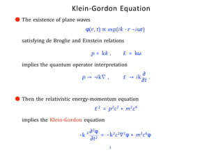
1. Klein-Gordon Equation
● The existence of plane waves
φ(r, t) ∝ exp(ik · r −iωt)
satisfying de Broglie and Einstein relations
p = kk , E = kω
implies the quantum operator interpretation
∂
p → −ik∇ , E → ik
∂t
.
● Then the relativistic energy-momentum equation
E 2 = p2c2 + m2c4
implies the Klein-Gordon equation
−k 2 ∂2φ
∂t2
1
= −k2c2∇2φ + m2c4φ

2. ● In covariant notation (see handout)
!
µ
µ
∂ ∂ +
mc
k
" #2
$
φ = 0
where
1 ∂2
∂µ ∂ = −∇
c2 ∂t2
2
µ 2
● KG wave function φ is a Lorentz-invariant (scalar) function; Lorentz
transformation r, t → r′, t′ implies φ → φ′ where
φ′(r′, t′) = φ(r, t) .
Hence it must represent a spin-zero particle (no orientation).
● Since |φ|2 is also invariant, this cannot represent a probability density. A
density transforms as time-like (0-th) component of a 4-vector, due to Lorentz
contraction of volume element.

3. ● Correct definition of density follows from the continuity equation:
∂ρ
∂t
= −∇ · J
(J = corresponding current vector), i.e.
∂ µ J µ = 0
where J µ = (cρ, J ) is the 4-current.
● We can obtain an equation of this form from the KG equations for φ and φ∗,
ik φ
%
∗∂ φ
∂t2
∂ φ
2 2 ∗
—
φ
∂t2
&
&
2 ∗ 2 2
' ∗(
= ikc φ ∇ φ −φ∇ φ ,
ik
∂
∂t
%
φ∗∂φ
∂t
—
φ
∂φ∗
∂t
= ikc2∇ · (φ∗∇ φ −φ∇ φ∗) .
Hence
%
∗
—
φ
∗
∂φ ∂φ
∂t ∂t
3
&
−ikc2 (φ∗∇ φ −φ∇ φ∗)
ρ = ik φ
J =
i.e. J µ = ikc2(φ∗∂µ φ −φ∂µ φ∗).

4. 4
● Normalization is such that the energy eigenstate φ = Φ(r)e−iEt/k has
ρ = 2E|Φ|2. Thus |Φ| = 1corresponds to 2E particles per unit volume
(relativistic normalization).
● Compare with Schr¨doinger current
S
J = −
ik
2m
(φ∗∇ φ −φ∇ φ∗) =
1
2mc2 J K G
which thus has in fact E/mc2 particles per unit volume.

5. 5
Problems with Klein-Gordon Equation
1. Density ρ is not necessarily positive (unlike |φ|2) ⇒ equation was rejected
initially.
2. Equation is second-order in t ⇒ need to know both φ and ∂φ
∂t
at t = 0 in order
to solve for φ at t > 0. Thus there is an extra degree of freedom, not present in
the Schro¨dinger equation.
3. The equation on which it is based (E2 = p2c2 + m2c4) has both positive and
negative solutions for E .
● Actually these problems are all related, since a solution φ = Φ(r)e∓iEt/k has
ρ = ±2E|Φ|2, and so for the general solution
φ = Φ+(r)e−iEt/k + Φ−(r)e+iEt/k
ik ∂φ
E ∂t .
t= 0
= Φ+ −Φ− are needed in order to
both φ(t = 0) = Φ+ + Φ− and
specify Φ+ and Φ−.

6. E lectromagnetic Waves
● In units where ϵ0 = µ0 = c = 1 (‘Heaviside-Lorentz’) Maxwell’s equations are
∂B
∇ · E = ρem , ∇ × E = −
∂t
∇ · B = 0 , ∇ × B = J em +
∂E
∂t
where (ρem, Jem) = J µ is the electromagnetic 4-current.
em
● In terms of the scalar and vector potentials V and A,
∂A
E = −
∂t
−∇V , B = ∇ × A .
So we find
∇ × (∇ × A 2
em
) ≡ ∇ ( ∇ · A) −∇ A = J −
∂2 A
∂t2
∂V
—
∇
∂t
6
● In terms of the 4-potential A µ = (V, A )
ν
ν µ µ
(∂ ∂ )A −∂ ( ν
ν
∂ A ) ν
≡ ∂ F νµ
= J µ
em

7. 7
where the electromagnetic field-strength tensor is
F νµ = ∂νA µ −∂µ A ν = −F µ ν .
● E and B , and hence Maxwell’s equations, are invariant under gauge
transformations
Aµ → A′µ = Aµ + ∂µ χ
where χ(r, t) is an arbitrary scalar function.
● Therefore wecan always choose Aµ such that ∂µ Aµ = 0 (Lorenz gauge). If
∂µ A µ = f /= 0, we can change to A ′µ = A µ + ∂µ χ where ∂µ ∂µ χ = −f .
● Then in free space (J µ = 0) we have ∂ν∂νA µ = 0.
❖ Massless KG equation for each component of Aµ
❖ Aµ is ‘wave function’ of photon
❖ Aµ is a 4-vector ⇒ photon has spin 1.
● Plane wavesolutions Aµ = εµ exp(ik · r −iωt) ≡ εµe−ik·x where εµ =
polarization 4-vector, k · x ≡ kµ xµ , kµ = (ω, k) = wave 4-vector.

8. ● From wave equation k · k = 0hence ω2 = k2
, i.e. E 2 = p2c2 (massless
photons).
● From Lorenz gauge condition ε · k = 0 ⇒ ε0 = ε · k/ω.
● Polarization 4-vector ε′µ = εµ + akµ is equivalent to εµ for any constant a.
Hence wecan always choose ε0 = 0. Then Lorenz condition becomes
transversity condition: ε · k = 0.
● E.g. for k along z-axis wecan express εµ in terms of plane polarization states
εµ = (0, 1, 0, 0) , εµ = (0, 0, 1, 0) ,
x y
R ,L
or circular polarization states εµ
= (0, 1, ± i, 0)/
√
2.
8
N.B. only 2 polarization states for real photons.

9. 9
Electromagnetic Interactions
● As in classical (and non-relativistic quantum) physics, weintroduce e.m.
interactions via the minimal substitution in the equations of motion:
E → E −eV , p → p −eA
i.e.
pµ → pµ −eA µ , ∂µ → ∂µ + ieAµ
● The Klein-Gordon equation becomes
(∂µ + ieAµ)(∂µ + ieAµ)φ + m2φ = 0 ,
(∂µ∂µ + m2)φ = −ie[∂µ(Aµφ) + Aµ(∂µφ)] + e2AµAµφ
The conserved current is now (k = c = 1)
J µ = i(φ∗∂µ φ −φ∂µ φ∗) −2eA µ φ∗φ

10. Klein Paradox
R e−ipx−iEt B e−ip’x−iEt
● Consider KG plane waves incident on electrostatic barrier, height V , width a
V
eipx−iEt A eip’x−iEt T eipx−iEt
x=0 x=a
KG equation for x < 0, x > a gives E 2 = p2 + m2
⇒ p = +
√
E 2 −m2
(sign from B.C.).
● In 0 < x < a, A µ = (V, 0) and so (E −eV )2 = p′2 + m2
⇒ p′ = +
√
(E −eV −m)(E −eV + m)
(sign choice is arbitrary since weinclude ±p′).
10

11. ● Matching φ and ∂φ/∂x at x = 0 and a gives (as for Schro¨dinger equation)
2
.
.
′
|T | = cosp a −
p′
i p p
2
′
p
11
% &
′
+ sin p a.
−2
.
● Now consider behaviour as V is increased:
❖ eV < E −m: p′ is real, |T | < 1 (|T | = 1when p′a = nπ).
❖ E −m < eV < E + m: p′ is imaginary, |T | < 1, transmission by tunnelling.
❖ eV > E + m: p′ is real again! |T | = 1 when p′a = nπ!?
● Note that when eV > E + m density inside barrier is negative:
ρ′ = 2(E −eV )|φ|2 < −2m|φ|2
● Meanwhile, the current inside remains positive, Jx
′ = 2p|T |2 (current
conservation). Hence when eV > E + m there is a negative density flowing
from right to left, giving a positive current. We interpret this as a flow of
em
antiparticles: J µ = eJµ always.

12. ● When eV > E + m and |T | = 1, antiparticles created at the back of the barrier
(x = a) travel to x = 0 and annihilate the incident particles. At the same time,
particles created at x = a travel to x > a, replacing the incident beam.
E E=0 E
12
+ +

● Antiparticles are trapped inside the barrier, but field is zero there, so there can
be perfect transmission for any thickness.

13. ● Antiparticles are like particles propagating backwards in time
x
t
+
+
+
x
13
t
+ +
−
eV > E+m
eV < E−m

14. 14
Charge Conjugation
● If φ is a negative-energy plane-wave solution of the KG equation, with
momentum p, φ = exp(ip · r + iE t) (E > 0), then φ∗ = exp(−ip · r −iE t) is a
positive-energy wave with momentum −p. Furthermore, in e.m. fields, φ∗
behaves as a particle of charge −e:
(∂µ + ieAµ)(∂µ + ieAµ)φ + m2φ = 0
⇒ (∂µ −ieA µ )(∂µ −ieA µ )φ∗ + m2φ∗ = 0
● Thus if φ is a negative-energy solution, wetake it to represent an antiparticle
with wave function φ∗(and hence positive energy, opposite charge and
momentum).
● Correspondingly, KG equation is invariant w.r.t. φ → φ∗, e → −e. This is
called charge conjugation, C.
N.B. Under C, J µ → −Jµ as expected.

15. 15
Electromagnetic Scattering
● We assume (for the moment) the same formula as in NRQM for the scattering
amplitude in terms of the first-order perturbation due to e.m. field:
A f i
by parts
= −i
∫
φ∗
f {ie[∂µ (A µ φi ) + A µ (∂µ φi )]}d4x
= A µ [φ∗
f (∂µ φi ) −(∂µ φ∗
f )φi ]d4x
e
∫
f i
= −ie
∫
A µ J µ
d4x
where J µ
= i ∗ µ
[φ (∂ φ µ ∗
f i f f
) −(∂ φ )
i i
φ ] is generalization of µ
f
J to φ =
/ φi
f i
(transition current). Note that to get A to order 1
e we only need J µ
f i to
order e0. Similarly, for Aµ we can use the free-field form
Aµ = εµe−ik·x
● For plane waves, φf ,i = e−i pf , i ·
x ,
J µ
f i
= (pi + pf )µ ei (pf −pi )·
x

16. Hence
A f i ei (pf −pi −k )·
x d4x
= −ieεµ(pi + pf )µ
∫
= −ie(2π)4ε · (pi + pf ) δ4(pf −pi −k)
● This corresponds to the Feynman rules for the diagram
p
p
k f
i
❖ An overall factor of (2π)4 δ4(pf −pi −k) (momentum conservation)
❖ εµ for an external photon line
❖ −ie(pi + pf )µ for a vertex involving a spin-0 boson of charge e.
N.B. 4-momentum cannot be conserved in this process for free particles! But
weshall seethat it can occur as part of a more complicated process, e.g.
particle-particle scattering by photon exchange.
16

17. ● We shall consider process ab → ab as scattering of a in e.m. field of b (both
spin-0).
f i
A = −ie a
∫
µ
A J µ
a' a d4x
a
p
a p’
b
p’
q=p’−p
b b
p
b
● Then (in Lorenz gauge) Aµ satisfies
17
ν b
∂ ∂ν Aµ = e J µ
b' b
N.B. We assume correct source current is
J µ
b' b b
= (p + pb e
'
b b
′ )µ i(p −p )·x

18. ● Solution for 4-vector potential is then
µ 1
q2
A = − e (p
b b b
+ p′
)µ ei q·
x
where q = pb
′ −pb and q2 = q · q.
● Hence
A f i =
q2
ieaeb
(pa a b
+ p′ ) · (p + pb
∫
′ ) ei (p'
a + pb
' −pa −pb )·
x d4x
a
= [−ie(p + pa
′ )µ
]
!
−ig µ ν
q2
18
$
[−ie b b
(p + p′ )ν]
× (2π)4δ4(p′
a + p′
b −pa −pb)
N.B. symmetry in a, b.
● Thus wehave the additional Feynman rule:
❖ −igµ ν/q2 for an internal photon line.

19. ● In processes involving antiparticles, remember weuse particles with opposite
energy and momentum; pµ = −p¯µ.
p
a
−
p
q
a
“pi ”=pa, “pf ”=−p¯a, “k”=−q,
A f i = −iea (2π)4ε · (pa −p̄a )δ4(q −pa −p̄a )
p
p
b
b
−
q
“pi”=−p¯b, “pf ”=pb, “k”=q,
A f i = −ieb(2π)4ε · (pb −p̄b)δ4(pb + p̄b −q)
19

20. ● Annihilation process
b
p
b
a
p
a
−
p p
−
q
eaeb
A f i = i
q2 (p −p 4 4
a a b b b b
¯ ) · (p −p̄ )(2π) δ (p + p̄ −q)
where q = pa + p¯a= pb + p¯b.
● Since wehave already normalized to 2E particles per unit volume, we have
A f i = M f i (2π)4δ4(
Σ
pf −
Σ
pi )
eaeb
where M f i is the invariant matrix element (see handout).
● Thus e.g. for annihilation process
M f i = i
q2 (pa −p̄a ) · (pb −p̄b)
20

21. ● In terms of the Mandelstam variables
s = (pa + p¯a)2 = q2
t = (pb −pa )2 = (p̄a −p̄b)2
u = (pa −p̄b)2 = (p̄a −pb)2
we get
M f i = i
eaeb
s
(u −t)
and hence the invariant differential cross section is
= a b
dσ e e (u −t)
2 2 2
dt 64πs3(p∗
a)2
∗
a
where p =
√
2
21
a
s/4 −m = c.m. momentum of a.

22. Dirac Equation
● Historically, Dirac (1928)waslooking for a covariant waveequation that was first-
order in time, to avoid the above ‘problems’ of the Klein-Gordon equation:
ik
∂ψ
∂t
2
= βmc ψ −ikc α · ∇ ψ ≡ H D irac ψ
● We want ψ also to satisfy KG equation ⇒ β, αx, αy, αz are matrices. Setting
k = c = 1:
∂2ψ
—
∂t2
= βmi
∂ψ
+ α · ∇
∂ψ
∂t ∂t
=
=
22
β2m2ψ −im(βα + α β) · ∇ ψ −(α · ∇ )2ψ
m2ψ −∇2ψ (KG equation)
Hence β2 = α2 = α2 = α2 = 1 and βαj + αj β = αj αk + αk αj = 0 for all
x y z
j /= k = x, y, z. This means that β, αx, αy, αz are (at least) 4 × 4 matrices.

23. ● A suitable representation is
β =
1 0
≡
I 0
0 −I
j
α =
0 0
0 1 0 0
0 0 −1 0
0 0 0 −1
0 σj
σj 0
23
x
σ =
0 1
1 0
where σj are the Pauli matrices:
y
, σ =
0 −i
i 0
z
, σ =
1 0
0 −1

24. 24
● Then ψ is represented by a 4-component object called a spinor (not a 4-vector!)
ψ1
ψ2
ψ =
ψ3
ψ4
N.B. Each component ψ1,2,3,4 satisfies the KG equation.
● For a particle at rest, ψ = φexp(−imc2t/k), Dirac equation ⇒ φ = βφ, and so
φ1
φ =
φ2
0
0
where φ1,2 tell us the spin orientation.

25. 25
● For antiparticle at rest, ψ = φe+ i m c2t/ k ⇒ φ = −βφ, so
φ =
0
0
φ3
φ4
where φ3,4 now give spin orientation.

26. Spin of Dirac Particles
● How do weprove that Dirac equation corresponds to spin one-half? We must
show that there exists an operator S such that J = L + S is a constant of
motion, and (k = 1) S 2
= S (S + 1) = 3 I .
4
● Note first that L = r × p is not a constant of motion:
H =
[Lz , H] =
=
In general, [L, H ] = iα × p /= 0.
βm + α · p
[x, H ]py −[y, H ]px
iαx py −iαy px .
● Thus we need [S , H ] = −iα × p.
2
This is true if S = 1
Σ where
j
Σ =
σj 0
0 σj
26
x y z
= −iα α α α .
x y z
4 4
Then S2
= 1 (Σ2 + Σ2 + Σ2) = 3 I , proving that S = 2
1
.

27. 27
Magnetic Moment
2
● In an electromagnetic field we make the usual minimal substitutions:
H → H −eV , p → p −eA
in the Dirac equation, to obtain
H = α · (p −eA ) + βm + eV
● Note that weno longer get the KG equation when we “square”:
Σ
(H −eV ) = α
j ,k
j k j j k k
α (p −eA )(p −eA ) + m2
= (p −eA )2 + m2 −e
Σ
j ,k
j k j k j k j k
(α α p A + α α A p )
Now for j /= k,
αj αk
εj k l Σ l ∇ j A k
= iεj k l Σ l , pj A k = A k pj −i∇ j A k
= Σ · (∇ × A) = Σ · B

28. 28
Hence
(p −eA )2 + m2 −eΣ · B
(H −eV )2 =
H −eV * m + 2
(p −eA) −
1 e
2m 2m
Σ · B
● This corresponds to a magnetic moment
m
µ =
e
S = ge
" e #
2m
S
where ge = 2 (experiment ⇒ 2.0023193. . . ).

29. 29
Dirac Density and Current
● Write Dirac equation as
∂ψ
∂t
= −imβψ −α · (∇ ψ)
● Transpose and complex conjugate:
∂ψ
∂t
†
†
= + imψ β −( †)
∇ψ · α
N.B. β, α are hermitian. Hence
∂
∂t
†
(ψ ψ) = −∇ †
(ψ αψ)
● Thus wecan take
ρ = ψ†ψ ≡ |ψ1|2 + |ψ2|2 + |ψ3|2 + |ψ4|2
J = ψ†αψ

30. 30
N.B. Density ρ is positive definite! This is what Dirac wanted, but it is really a
problem – what about antiparticles?!
● Answer will not come until welearn some quantum field theory.

31. 31
C ovariant Notation
● Nobody uses α and β any more. Instead we define γ-matrices:
γ0 = β , γj = βαj (j = 1, 2, 3)
⇒ γµ γν + γνγµ ≡ {γµ , γν} = 2gµ ν. Also define
ψ̄ ≡ ψ†β = (ψ1
∗, ψ2
∗, −ψ3
∗, −ψ4
∗)
in usual (‘Bjorken and Drell’) representation. Then
ρ = ψ†ψ = ψ†β2ψ = ψ¯γ0ψ
J = ψ†αψ = ψ†β2αψ = ψ¯γψ
and J µ is a 4-vector:
J µ = (ρ, J) = ψ¯γµψ

32. 32
● We can also show that
ψ̄ψ = |ψ1|2 + |ψ2|2 −|ψ3|2 −|ψ4|2
transforms like a scalar (invariant) under Lorentz transformations.
● Multiplying through by β, Dirac equation becomes
iγ0 ∂ψ
∂t
j
j
= mψ −iγ ∇ ψ
Hence
(γµ∂µ + im)ψ = 0
(γµpµ − m)ψ = 0

33. Free-Particle Spinors
u =
φ
χ
φ
=
2
φ1
● A positive-energy plane wave
ψ = u(E , p) exp(ip · r −iE t)
satisfies (γµ pµ −m)u = 0. Writing
χ1
χ2
this means that
33
E −m −σ · p φ
+ σ · p −E −m χ
= 0
Thus χ =
σ · p
φ
E + m

34. ● Remember that
2
S = 1
Σ = 1
2
σ
0
0
34
σ
Hence
φ = N
1
0
for spin up (along z-axis)
= N
0
1
for spin down
We have also
σ · p
1
=
0 px + ipy
pz ,
1
σ · p
0
=
px −ipy
−pz

35. Thus
↑ =
u N
1
0
pz
p x + i p y
E + m
E + m
, ↓ =
u N
0
1
px −i py
−pz
E + m
E + m
.
❖ Normalization is as usual ρ = ψ†ψ = u†u = 2E particles per unit volume.
This gives
N 2
1+
2 2
x y
p + p + p2
z
(E + m)2
3 4
= 2E
Using p2 = E 2 −m2 gives N =
√
E + m.
❖ Notice that the ‘small’ (3,4) components are O(v/c) relative to ‘large’ ones
(1,2).
● For antiparticle of 4-momentum (E, p) weneed solution with pµ → (−E, −p):
ψ = v(E , p) exp(−ip · r + iE t)
35

36. From the Dirac equation we now find
−E −m σ · p φ
36
−σ · p E −m χ
= 0
Thus
E + m
φ =
σ · p
χ
● Like 4-momentum, spin must be reversed, so
v↑ = N
px −ipy
E + m
−pz
E + m
0
1
, v↓ = N
pz
E + m
px + i py
E + m
1
0
.

37. 37
Charge Conjugation
● Like the KG equation, the Dirac equation has charge conjugation symmetry. If
ψ is a negative-energy solution, there is a transformation
c ∗
ψ → ψ = Cψ
such that ψc is a positive-energy solution for charge −e. To find C:
γµ(∂µ + ieAµ)ψ + imψ = 0
⇒ γ∗
µ (∂µ −ieA µ )ψ∗ −imψ∗ = 0
⇒ −C γ∗
µ C −1(∂µ −ieA µ )ψc + imψc = 0 .
Hence weneed Cγ∗µC−1 = −γµ, i.e. γµ C = −Cγ∗µ.

38. 38
● Since all γµ are real except γ2 (which is pure imaginary) in our standard
representation, wecan take
C = iγ2 =
0 0
0 0 0 1
0 0 −1 0
−1 0
1 0 0 0
Explicitly, for free particles, v↑c = u↑, v↓c = −u↓

39. 39
Parity Invariance
● Similarly if ψ(r, t) is a solution of the Dirac equation, there exists a
transformation
ψ(r, t) → ψP (r, t) = P ψ(−r, t)
such that ψP is also a solution. Now
γ0 ∂
∂t
r, t) = 0
% &
%
0 ∂
∂t
—
γ · ∇ + im ψ(
+ γ
&
· ∇ + im ψ(−r, t) = 0
%
⇒ γ
⇒ P γ P
0 −1 ∂
∂t
−1
+ P γP · ∇ + im ψ
&
P
(r, t) = 0 .
Hence we need P γ0P −1 = γ0 , P γP −1 = −γ ,
i.e P γ0 = γ0P , P γj = −γj P (j = 1, 2, 3)

40. 40
● These relations are satisfied by
P = γ0 =
1 0
0 0
0 1 0 0
0 0 −1 0
0 0 0 −1
● For a particle at rest,
ψ = u(m, 0) e−i m t ,
but for an antiparticle at rest
ψ = v(m, 0) e+ i m t ,
ψP
= +ψ
ψP
= −ψ
Thus particle and antiparticle have opposite intrinsic parity.
● Notice that for KG equation the parity transformation is simply
φ(r, t) → φP (r, t) = φ(−r, t)

41. i.e. φ is a true scalar function, since
%
%
∂2
∂t2
2
—∇ + m
2
&
φ(r, t) = 0
⇒
∂2
∂t
41
2
2
—
∇ + m φ(−r, t) = 0
2
&
● For the Dirac equation, the scalar is not ψ but
Φ = ψ¯ψ = ψ†γ0ψ
Check:
Φ(r, t)
ΦP (r, t)
= ψ†(r, t)γ0ψ(r, t)
= ψ†(−r, t)γ0†γ0γ0ψ(−r, t)
= ψ†(−r, t)γ0ψ(−r, t)
= Φ(−r, t)

42. ● Similarly, J µ is a true vector:
Jµ(r, t) = ψ†(r, t)γ0γµψ(r, t)
JP µ(r, t) = ψ†(−r, t)γ0†γ0γµγ0ψ(−r, t)
But γ0†γ0γµγ0 = γµγ0 = γ0γµ for µ = 0, = −γ0γµ for µ = 1, 2, 3. Hence, as
expected for a true vector,
J P 0(r, t) = J 0(−r, t) , J P
(r, t) = −J (−r, t) .
● Weak interactions involve the axial current
A
J µ
= ψ¯γµγ5ψ
where
γ5 = iγ0γ1γ2γ3 =
0 I
42
I 0
in our standard representation.

43. 43
A
● Under parity transformations J µ
is an axial vector:
J P µ
A
†( µ 5 0
(r, t) = ψ −r, t)γ γ γ ψ(−r, t)
Now γ5γ0 = −γ0γ5 (actually γ5γµ = −γµγ5 for all µ = 0, 1, 2, 3), so
A
J (
P 0 0
r, t) = −J (−r, t) , P
A
J (r, t) = J (−r, t)
as expected for an axial vector.
● Similarly ΦP = ψ¯γ5ψ is a pseudoscalar
P
ΦP (r, t) = ψ†(−r, t)γ5γ0ψ(−r, t)
= −ψ̄(−r, t)γ5ψ(−r, t)
= −ΦP (−r, t)

44. Massless Dirac Particles
φ
● For m = 0 the positive-energy free particle solutions are
ψ = u(E , p) exp(ip · r −iE t)
χ
where E = |p| and so u = gives
44
|p| −σ · p φ
σ · p −|p| χ
= 0
Hence χ = Λφ where Λ = σ · p/|p| is the helicity operator: Λ = ±1 for spin
aligned along/against direction of p (‘right/left-handed’)
● Note that if ψ represents a massless particle then
φ
γ5ψ =
Λφ
= Λψ (Λ2 = 1)

45. 45
● Hence γ5 is the helicity operator for massless particles (minus helicity for
massless antiparticles).
● Weak interactions are ‘V–A’, i.e. they involve the current
µ µ
A f i
(J −J ) = ψ̄f γµ (1 −γ5)ψi
If i is a massless particle, then (1 −γ5)ψi vanishes for helicity +1, i.e. only
left-handed states interact. The same applies to particle f , since
ψ̄f i
†
f
γ (1 −γ )ψ = ψ γ (1 + γ )
µ 5 0 5 µ 5
γ ψ = (1 −γ )
5 6
† 0 µ
ψ γ γ )ψ
i f i
❖ Thus if neutrinos are massless, only left-handed neutrinos (right-handed
antineutrinos) interact.
❖ In the Standard Model, neutrinos are massless and right-handed neutrinos
do not exist.
❖ This is consistent with relativity, because helicity is frame-independent for
massless particles.
❖ In reality neutrinos do have mass, so both helicities must exist, but the
right-handed states interact more weakly (as for electrons).

46. 46
Electromagnetic Interactions
● We already saw that in an e.m. field Dirac Hamiltonian is
H = α · (p −eA ) + βm + eV
= H0 + eγ0γµAµ
where H0 is the free-particle Hamiltonian.
● Hence first-order perturbation theory gives a transition amplitude
A f i f
= −i
∫
ψ†
(eγ0γµ A µ )ψi d4x
f i
= −ie
∫
J µ
Aµ d4 x
where J µ
= ψ̄f γµ ψi .
f i
● For plane waves, ψf,i = uf,ie−ip·x, and so the only difference from the KG
(spin zero) case is that weneed a vertex factor of
−ieūf γµ ui
for spin one-half instead of −ie(pf + pi)µ for spin 0.

47. ● Invariant matrix element is
M f i =
ieaeb
q2
(ūa' γµ
ua )(ūb' γµ ub)
a
p
a
p
b
p’
b
p’
q=p’−p
b b
Hence
47
f i
| M |2
=
e2 e2
a b
t2
L L
µ ν b
a µ ν
where
Lµ ν
a = (ūa' γµ ua )(ūa' γνua )∗
= (ūb' γµ ub)(ūb' γνub)∗
Lb
µ ν

48. 48
● For given spin states of a, b,a′ and b′, wecan evaluate these tensors explicitly
using the above expressions for free-particle spinors. However, we often
consider unpolarized scattering, when wehave to average over initial and sum
over final spin states. Then
a
Lµ ν = 1
2
Σ
spins
'
a a
(ū γ u )( a'
ū γ ua
µ ν )∗
and similarly for Lb
µ ν. This can be evaluated using the algebra of the
γ-matrices.

49. 49
Gamma Matrix Algebra
● The tensor
a
Lµ ν = 1
2
Σ
'
µ
'
(ū γ u )(ū γ u
a a a a
ν )∗
spins
can be expressed in terms of traces of products of γ-matrices, using
Σ
µ
µ
uu¯ = u↑u¯↑ + u↓u¯↓ = γ p + m
spins
We also have
'
ν
a a
(u¯ γ u )∗= (
†
a' a a
0 ν † ν† 0
u γ γ u )∗ = u γ γ ua' a
ν
= ū γ ua'
since γν†γ0 = γ0γν.
● Thus
a
Lµ ν = 1
2
Σ
a' spins
where we use Feynman’s notation /p = γµpµ. Putting in Dirac matrix indices,
ūα Γαβuβ = Tr(uūΓ). Hence
ūa' γµ (/pa + ma )γνua'
a
1
2
= Tr { a
Lµ ν ′ + a
µ
(/p m )γ ( a a
ν
/p + m )γ }

50. 50
kµkν
′ Lµ ν
a
1
2
1
2
= Tr
= Tr
{(/
p
a
′ + a a a
′
m )/k(/p +
m )/k }
′
a
{/p /
ka
′
/p /k }
+
1
2
2
a
m Tr {/k ′
′
a
= 2(p · kp ′ +
a a
′
a
′
· k p · kp · k −p a
′
a
· p k a
· k m k · k
/k }
′ + 2 ′)
(see examples sheet for last step).
● Removing the arbitrary vectors kµ and kν
′ ,
L µ ν
a
5
= 2 p p
a a
µ ′ν ′µ ν
a a a
+ p p −(p · p′
a a
—
m )g
2 µ ν
6
and similarly
Lb
µ ν
5
= 2 pbµ p′
bν bµ bν b
+ p′ p −(p · p′
b
2
b
—
m )gµ ν
so
L µ νL b
a µν = 8(pa b a
· p p · pb
′ ′ + a
p · p p
′ ′
b a b
2
a
· p −m p b · p′
b
2
b
—
m p
6
a a
2 2
a b
· p′ + 2m m )

51. ● Expressing this in terms of the Mandelstam invariants s, t and u, wefind an
invariant differential cross section
dσ
=
e2 e2
a b
dt 32πst2(pa
∗)2 a b a b
+ u2 −4( + )(s + u) + 6( + )
s2 m2 m2 m2 m2 2
5 6
● For processes involving Dirac antiparticles, weshould use the v-spinors in
place of u’s:
p
a
−
p
q
a
“ui ”= ua , “ūf ”= v̄a
′ ⇒ vertex factor −iev̄a
′ γµ ua .
a
p
−
a
−
p ’
q
“ui”=va
′ , “u¯f ”=v¯a ⇒ vertex factor −iev¯aγµva
′ .
51

52. 52
● We also need
Σ
spins
N.B. Different sign of m!
↑
vv¯ = v v ↓
¯↑ + v v̄↓ = /p −m
a a
● Note, however, that the tensor Lµ ν only involves m2 . Replacing a by a¯
reverses sign of ma, which does not affect the (unpolarized) scattering cross
section. Hence ab, a¯b,a¯band a¯¯bscattering (by single photon exchange) are all
the same.

53. Compton Scattering
’
p+k
’
+

k k’
p−k’
k

k’
p p’ p p’
● In the Compton scattering process γ + e → γ + e, weneed the propagator
factor for a virtual Dirac particle. This is
i
q2 −
m2
Σ
spins
uu¯ =
i(/q + m
)
q2 −m2
● Compare with photon propagator
i
q2
Σ
spins
µ ν
ε ε∗“ = ”
µ ν
i(−g )
q2
53

54. Thus the two graphs give M f i = M 1 + M 2 where
1
′
ν
ε u ν
¯′(−ieγ )
i(/p + /k + m
)
(p + k)2 −m2
µ
(−ieγ )uεµ
2 µ
µ
M =
M = ε u¯′(−ieγ )
′
i(/p −/k
+ m)
(p −k′)2 −m2
54
(−ieγ )uε
ν ′
ν
● The relative phase is +1 because the graphs differ by exchange of identical
bosons.
● For the unpolarized case, wewant to average over initial spin states and sum
over final ones. We know how to do this for the electrons. For the photons,
consider the incoming polarization εµ. We can write schematically
spins ε=εx ,εy
where the tensor Mµ λ is to be determined. However, we know that it must
have the properties kµ Mµ λ = kλ Mµ λ = 0 to ensure gauge invariance, which
allows us to replace εµ → εµ + akµ for any a.
1 2
2
| M + M | =
Σ Σ
εµ ε∗
λ M µ λ

55. ● Choose z-axis along k: kµ = |k|(1, 0, 0, −1). Then above property implies
M 00 = M 03 = M 30 = M 33, while
Σ
ε=εx ,εy
εµ ελ
∗M µ λ
= M 11 + M 22
M 11 + M 22 + M 33 −M 00
µ
=
= −M = − µ λ
g M
µ µ λ
● Thus, due to gauge invariance, wecan replace photon polarization sum by
−gµλ.
● Applying the same trick to the outgoing photon polarization (εν
′) sum, wefind
a contribution from the first diagram of
1
4
Σ
spins
2
|M1| =
e4
4(s −m )
55
2 2
′ ν
Tr {(/p+ m)γ (/p + /k +
m
)
µ
γ (/p + m)γµ(/p + /k + m)γν
}

56. s2
e4
Tr
{/p /
p
( + /k /
p
) ′(/p + /k
}
● In the extreme relativistic limit (s, |t|, |u| + m2), this becomes (using results
on examples sheet)
e4
) = 8 (p · k)(p′ · k)
s2
56
= −2e 4
u
s
● Other diagram and interference terms are left as an exercise.