The document discusses group theory and its applications in physics. It begins by introducing symmetry groups that are important in physics, including translations, rotations, and Lorentz transformations. It then discusses the use of group theory in formulating fundamental forces and the Standard Model of particle physics. The document provides definitions of group theory concepts like groups, operations, identity, and inverse. It explains how group theory provides a mathematical framework for describing physical symmetries.

1. From First Principles
PART VI – GROUP THEORY
June 2017 – R4.0
Maurice R. TREMBLAY
The E8 (with thread made by
hand) Lie group is a perfectly
symmetrical 248-dimensional
object and possibly the
structure that underlies
everything in our universe.

2. Group theory provides the natural mathematical language to formulate symmetry
principles and to derive their consequences in Mathematics and in Physics. Although we
will not be proving it, the special functions of mathematical physics (e.g., spherical
harmonics, Bessel functions, &c.) invariably originate from underlying symmetries and
representations found in group theory problems. The main subject here is, however, the
mathematics of group representation theory, with all its inherent simplicity and elegance.
2017
MRT
The outline is as follows: Standard group representation theory; basic elements of
representation theory of continuous groups in the Lie algebra approach (without going
into the details of how Lie algebras come about) by studying the one-parameter rotation
and translation groups; treatment of the rotation group in three-dimensional space (i.e.,
SO(3)); explore basic techniques in the representation theory of inhomogeneous groups
and; finally, offer a systematic derivation of the finite-dimensional and the unitary repre-
sentation of the Lorentz group, and the unitary representation of the Poincaré group.
The Poincaré group embodies the full continuous space-time symmetry of Einstein’s
special relativity which underlies pretty much all of contemporary physics. The relation
between finite-dimensional (non-unitary) representations of the Lorentz group and the
(infinite-dimensional) unitary representation of the Poincaré group is discussed in detail
in the context of relativistic wave functions, field operators and wave equations.
In geometrical and physical applications, group theory is closely associated with
symmetry transformations of the system under study. The theory of group representation
provides the natural mathematical language for describing symmetries of the physical
world, and most importantly, in whatever number of dimensions we deem necessary!
Forward
2

3. Contents
2017
MRT
PART VI – GROUP THEORY
Symmetry Groups of Physics
Basic Definitions and Abstract Vectors
Matrices and Matrix Multiplication
Summary of Linear Vector Spaces
Linear Transformations
Similarity Transformations
Dual Vector Spaces
Adjoint Operator and Inner Product
Norm of a Vector and Orthogonatility
Projection, Hermiticity and Unitarity
Group Representations
Rotation Group SO(2)
Irreducible Representation of SO(2)
Continuous Translational Group
Conjugate Basis Vectors
Description of the Group SO(3)
Euler Angles α, β & γ
Generators and the Lie Algebra
Irreducible Representation of SO(3)
Particle in a Central Field
Transformation Law for Wave Functions
Transformation Law for Operators
Relationship Between SO(3) and SU(2)
Single Particle State with Spin
Euclidean Groups E2 and E3
Irreducible Representation Method
Unitary Irreducible Representation of E3
Lorentz and Poincaré Groups
Homogeneous Lorentz Transformations
Translations and the Poincaré Group
Generators and the Lie Algebra
Representation of the Poincaré Group
Normalization of Basis States
Wave Functions and Field Operators
Relativistic Wave Equations
General Solution of a Wave Equation
Creation and Annihilation Operators
References
“We need a super-mathematics in which the operations are as unknown as the quantities they operate on,
and a super-mathematician who does not know what he is doing when he performs these operations.
Such a super-mathematics is the Theory of Groups.” Sir Arthur S. Eddington, The World of Mathematics,
Volume 3, 1956.
3

4. We start by enumerating some of the commonly encountered symmetries in physics to
indicate the scope of our subject:
4
axxx ++++=→
2017
MRT
where a is a constant three-vector. This symmetry, applicable to all isolated systems, is
based on the assumption of homogeneity of space (i.e., every region of space is
equivalent to every other – in other words, physical phenomena must be reproducible
from one location to another). The conservation of linear momentum is a well known
consequence of this symmetry.
b) Translations in Time:
τ+=→ ttt
where τ is a constant scalar. This symmetry, applicable also to isolated systems, is a
statement of homogeneity of time (i.e., given the same initial conditions, the behavior of
a physical system is independent of the absolute time – in other words, physical
phenomena are reproducible at different times). The conservation of energy can be
easily derived from it.
a) Translations in Space:
1. Continuous Space-Time Symmetries:
Symmetry Groups of Physics
“Nature, it seems, does not simply incorporate symmetry into physical laws for æstetic reasons. Nature
demands symmetry.” Michio Kaku, Introduction to Superstrings, 1988, P. 4.

5. 5
2017
MRT
c) Rotations in three-dimensional Space:
∑=
=→⇔=→
n
j
ji
j
ii
xRxxR
1
xxx
where i,j=1,2,3, {xi} are the three-components of a vector, and R is a 3×3 (orthogonal)
rotation matrix. This symmetry reflects the isotropy of space (i.e., the behavior of
isolated systems must be independent of the orientation of the system in space). It leads
to the conservation of angular momentum.
d) Lorentz Transformations (i.e., rotations in 4D Minkowski space-time):






Λ→





x
v
x
tt
)(
and x stands for a three-component column vector and Λ(v) is the 4×4 Lorentz matrix:












−+−
−
=Λ
T
T
vv1
v
v
v
ˆˆ)1(
)]([
γ
γ
γ
γ
µ
ν
c
c
where γ =1/√(1−|v|2/c2), v is the velocity vector (i.e., a column vector), vT is its transpose
(i.e., a row vector) and v is its unit vector. This symmetry embodies the generalization of
classical (i.e., Newtonian) physics where separate space and time symmetries are
rolled up into a single space-time symmetry, now known as Einstein’s special relativity.
ˆ

6. 2. Discrete Space-Time Symmetries:
6
2017
MRT
xxx −=→
This symmetry is equivalent to the reflection in a plane (i.e., mirror symmetry), as one
can be obtained from the other by combining with a rotation through and 180° angle (or
π). Most interactions in nature obey this symmetry, but the weak interactions (i.e., the
ones responsible for radioactive decays and other weak processes) does not.
b) Time Reversal Transformation:
ttt −=→
This is similar to the space inversion and this symmetry is respected by all known forces
except is isolated instances (e.g., neutral K-meson decay) which are not yet well-
understood.
a) Space Inversion (or Parity transformation):
c) Discrete Translations on a Lattice:
bnxxx +=→
where b is the lattice spacing and n is an integer.

7. d) Discrete Rotational Symmetry of a Lattice (Point Groups): These are subsets of
the three-dimensional rotation- and reflection-transformations which leaves a given
lattice structure invariant.
7
2017
MRT
In conjunction with the discrete translations (c), they form the space groups which
are the basic symmetry groups of solid state physics.
Classification of the 32 Crystallographic Point Groups
Cubic O , Oh , Td , T , Th
Tetragonal C4 , S4 , D2d , C4v , C4h , D4 , D4h
Hexagonal D3h , D6 , D6h , C3h , C6 , C6h , C6v
Trigonal C3v , D3d , D3 , C3 , S6
Rhombic C2v , D2 , D2h
Triclinic C1 , Ci (S2)
Monoclinic C1h (Cs) , C2 , C2h
The Schonflies notation is used above: C (cyclic), D (dihedral), O (octohedral), and T
(tetrahedral). Moreover, Cn (n rotations about an n-fold symmetry axis), S2n (2n rotary
reflections), Dn (n rotations of the group Cn and n rotations through an angle π about
horizontal axes), T (the group of proper rotations of a regular tetrahedron), &c.
Of these, point groups are defined as groups consisting of elements whose axes and
planes of symmetry have at least one common point of intersection. All possible
symmetry operations for point groups can be represented as a combination of a) a
rotation through a difinite angle about some axis and b) a reflection in some plane.
There are 32 crystallographic point groups (see Table).

8. 3. Permutation Symmetry:
8
2017
MRT
Systems containing more than one identical particle are invariant under the interchange
of these particles. The permutations form a symmetry group. If these particles have
several degrees of freedom, the group theoretical analysis is essential to extract
symmetry properties of the permissible physical states (e.g., Bose-Einstein and Fermi-
Dirac statistics, Pauli exclusion principle, &c.)
4. Gauge Invariance and Charge Conservation:
Both classical and quantum mechanical formulation of the interaction of electromagnetic
fields with charged particles are invariant under gauge transformation. This symmetry is
intimately related to the law of conservation of charge.
5. Internal Symmetries of Nuclear and Elementary Particle Physics:
The most familiar symmetry of this kind is the isotropic spin invariance of nuclear
physics. This type of symmetry has been generalized and refined greatly in modern day
elementary particle physics. All known fundamental forces of nature are now formulated
in terms of gauge theories with appropriate internal symmetry groups (e.g., the
SU(2)⊗U(1) theory of unified weak and electromagnetic interactions, and the SU(3)C
theory of strong interaction called Quantum Chromodynamics).

9. Group theory is important in formulating the Standard Model (SM) of particle physics
which is gravitation, together with SU(3)C⊗SU(2)L⊗U(1)Y gauge-invariant strong and
electroweak interactions. After the sponteneous breaking of the symmetry as a result of
the Higgs coupling, we are left with SU(2)L⊗U(1)EM as exact gauge symmetries, and the
gluons and the photons as massless particles. The Lagrangian Density is given by:
9
2017
MRT
44444 344444 21444 3444 21
44444444 344444444 21
4444444444444 34444444444444 21444444444 3444444444 21
HiggstocoulingsandmassesFermion
gluonsandquarksbetweennsInteractio
couplingsandmassesHiggsand,,,
fermionsofnsinteractiokelectroweaandenergiesKineticbosonsgaugetheofninteractioselfandenergyKinetic
SM
.).()(
)(
22
1
2
1
2224
1
4
1
4
1
21
2
chffGffGGqqg
VB
Y
gWgi
fB
Y
giffB
Y
gWgifGGBBWW
RcLRLa
a
as
ZW
i
i
i
RRLi
ii
La a
a
i i
i
++++
−





′−−∂+






′−∂+





′−−∂+−−=
∑
∑
∑∑∑
±
−
φφλγ
φφτ
γ
τ
γ
µ
µ
γ
µµµ
µµ
µ
µµµ
µµν
µν
µν
µν
µν
µνL
where g, g′, gs, and G1/2 are a coupling constants and Y (Q=T3 +Y/2) is the hypercharge. γ µ
are the gamma matrices. ττττ=τi (i=1,2,3) are Pauli’s ‘isospin’ 2×2 matrices. The SU(2)⊗U(1)
gauge group has four vector fields, three associated with the adjoint representation of
SU(2), which we denote by Wµ =Wi
µ (µ=0,1,2,3) in isospin space and one with U(1) denoted
by Bµ. qj (qk) is a quark (antiquark) field of flavor q=u,d,c,s,t,b and color j,k=1,2,3 or R, G,
B. The field strengths of the U(1) and SU(2) gauge fields are given by Bµν =∂µBν −∂ν Bµ and
Wµν =Wi
µν =∂µWi
ν −∂ν Wi
µ −gΣjkWj
µWk
ν , respectively. V(φ) is the sponteneous symmetry
breaking potential. Ga
µ are eight gluon field potentials (a=1,2,…,8) with λa being the eight
independent traceless and Hermitian,3×3 matrices of SU(3) and Hermitian conjugate (h.c.).
Q 3 2 1/6
UC 3 1 −2/3
DC 3 1 +1/3
L 1 2 −1/2
EC 1 1 +1
{ {
{
i
Ri
L
i
L
i
R
i
Ri
L
i
L
L
E
E
L
DU
D
U
Q
and
,,
:sSM
,,
,,,,








=








=
ν
τµe
bsdtcu
QUDLE
44 844 7648476 (EW)kElectroweaQCD
YLC )(U)(SU)(SUG 123 ⊗⊗=
_

10. A set {G:a,b,c,…} is said to form a group if there is an operation ‘⋅⋅⋅⋅’, called group
multiplication, which associates any given (ordered) pair of elements a,b∈G with a well-
defined product a⋅⋅⋅⋅b which is also an element of G, such that the following conditions are
satisfied:
10
2017
MRT
1. The operation ‘⋅⋅⋅⋅’ is associative, that is:
2. Among the elements of G, there is an element 1, called the identity, which has the
property that:
3. For each a∈G, there is an element a−1 ∈G, called the inverse of a, which has the
property that:
An Abelian group G is one for which the group multiplication is commutative:
for all a,b,c∈G.
cbacba ⋅⋅=⋅⋅ )()(
for all a∈G;
aa =⋅1
1=⋅=⋅ −−
aaaa 11
0=−⇔= abbaabba
for all a,b,c∈G. Note that the operation ‘⋅⋅⋅⋅’ is now understood as silent between terms.
The commutation operation, being a widely repeated operation especially in quantum
mechanics, is usually indicated by square brackets:
Basic Definitions and Abstract Vectors
],[ baabba =−

11. Here are a few definitions of vectors and vector indices:
11
n
n
n
i
i
i
xxxx eeeex ˆˆˆˆ 2
2
1
1
1
+++== ∑=
L
2017
MRT
2. Certain linear spaces have non-trivial invariant metric tensors, say gij. In that case, it
is convenient to distinguish between contravariant components of a vector labeled by an
upper index as above, and covariant components of the same vector labelled by a lower
index defined by:
∑∑ ==
==
n
j
j
jii
n
j
j
jii xgxxgx
11
and
such that the scalar product Σi xi yi is an invariant. The metric tensor for Euclidean
spaces is the Kronecker delta function: gij =δij . Hence, for Euclidean spaces, xi =xj.
3. Vectors in general linear vector spaces will be formally denoted by Greek or Latin
letters inside Dirac’s | 〉 (‘ket’) or 〈 | (‘Bra’) symbols (e.g., |x〉, |ξ 〉, …, or 〈 f |, 〈ψ |, … &c.)
4. Multiplication of a vector |x〉 by a number α can be written in three equivalent ways:
xxx ααα =⋅=
1. Vectors in ordinary two- or three-dimensional Euclidean spaces will be denoted by
boldface single Latin letters (e.g., x, y,…&c.) Unit vectors (i.e., vectors of unit length) will
be distinguished by an overhead caret (e.g., ê, u, z,…&c.) Basis vectors in n-
dimensional Euclidean space will be denoted by {êi ,i=1,2,…,n}. The components of x
with respect to this basis are denoted by {xi,i=1,2,…,n} where:
ˆ ˆ

12. 5. Lower indices are used to label ket basis vectors (e.g., {|êi 〉,i=1,…,n}); upper indices
are used to label components of ket-vectors. Consequently, if xi are components of |x〉
with respect to the set of basis states kets {|êi 〉}, then we have the ket-vectors:
12
2017
MRT
∑=
=
n
i
i
i
x
1
ˆex
6. Upper indices are used to label basis-vectors (e.g., {|êi 〉,i=1,…,n}); lower indices are
used to label components of bra-vectors:
∑=
=
n
i
i
ix
1
ˆex
The raising and lowering of the index in this way is a desirable convention, since the
scalar product can be written as:
∑=
=
n
i
i
i yx
1
†
yx
where † indicates that Hermitian conjugation of an arbitrary matrix xi which is obtained
by taking the complex conjugate, * (i.e., replacing i=√(−1) by −i) of the matrix, xi
* and
then the transpose, T (i.e., interchanging corresponding rows and columns), xi
*T, of the
complex conjugate matrix such that:
T*†
ii xx =

13. Elements of a matrix M will be labelled by a row index, j, followed by a column index, i,
as a mixed M j
i (second order) or, like a linear (first order) vector, can be represented in
covariant, Ck, contravariant, D j, forms. Matrices can be symmetric or antisymmetric:
13
2017
MRT
j
i
j
iijji SSSS == TT
or
The normal notation for matrix multiplication is:
∑∑=
k m
m
j
k
m
i
k
i
j CBACBA ][
Just as in the case of vector components, it is desirable to switch upper and lower
indices of a matrix when its complex conjugate is taken. As Hermitian conjugation also
implies taking the transpose, it is natural to incorporate also ST
i
j =S j
i, and arrive at the
convention:
*][*† i
j
i
j
i
j SSS ==
As indices may also be raised or lowered by contraction with the metric tensor,
variants of [ABC]i
j=Σkm Ai
k Bk
m Cm
j may look like:
∑∑ ==
mk
jm
mki
k
mk
m
jmk
kii
j CBACBACBA ][
Matrices and Matrix Mutiplication
The transpose of a matrix, indicated by the superscript T, implies the interchange of
the row and column indices. We write for the symmetric matrix Si j or for S j
i above:
j
i
j
iijji
j
i
j
iijji AAAASSSS −=−=== andorand

14. A linear vector space V is a set {|x〉,|y〉,…,&c.}, on which two operations ++++ (addition)
and ⋅⋅⋅⋅ (multiplication) are defined, such that the following basic axioms hold:
14
2017
MRT
1. If |x〉∈V and |y〉∈V, then:
2. If |x〉∈V and α is a real (or complex α =a+ib) number, then:
for all |z〉∈V.
zyx ≡++++
xxx ααα ≡⋅≡
for all |x〉∈V.
3. There exists a null vector |0〉, such that:
x0x =++++
for all |x〉∈V.
Summary of Linear Vector Spaces
4. For every |x〉∈V, there exists a negative ket-vector |−x〉∈V, such that:
0xx =−++++
5. The operation ++++ is commutative:
xyyx ++++++++ =
6. Multiplication by a trivial entity 1 (i.e., it doesn’t change anything – being trivial!):
xx1 =⋅
and associative:
zyxzyxzyx ++++++++++++++++++++++++ == )()(

15. 7. Multiplication by a number α is associative:
15
2017
MRT
xxx βαβαβα ≡⋅=⋅ )(
8. The two operations satisfy the distributive properties:
yxyxxxx αααβαβα ++++++++++++ =⋅=⋅+ )()( and
The numbers {xi} are the components of x with respect to the basis {êi}. Vector
spaces which have a basis with a finite number of elements are said to be finite
dimensional.

16. Linear transformations (e.g., using first-order operators) on vector spaces form the basis
for all analysis on vector spaces.
16
2017
MRT
VAV A
∈→∈ xx
A linear transformation (operator) A is a mapping of the elements of one vector space,
say V, onto those of another, say V, such that:
Now, if:
2211 xxy αα ++++=
for all |y〉∈V, then:
2211 xxy AAA αα ++++=
for all |Ay〉∈V.
xxx AAA
≡→
Linear Transformations
It is convenient to adopt the alternative notation |Ax〉=A|x〉, introduced by Dirac:
The reader that is not necessarily acquainted with vector spaces of this kind is truly
encouraged to first review and digest to some degree the first few chapters of P. A. M.
Dirac’s masterpiece: The Principles of Quantum Mechanics, Clarendon Press; Fourth
Edition edition (newer english 2012-2013 editions are now available via searches on
Amazon). I mean, guys like R.P. Feynman and S.Weinberg read it,understood it,and
later managed to ponder on their own formulation of quantum fields based on reading it!
_
_

17. Given any two vector spaces Vn and Vm with respective bases {êi ,i=1,…,n} and {êj ,j=
1,…,m}, every linear operator A from Vn to Vm can be represented by a m×n component
transformation matrix Aj
i. The correspondence is established as follows…
17
∑∑ ∑∑ ∑∑∑ =








=








====
= j
j
j
j
j
i
ij
i
i j
j
j
i
i
i
i
i
n
i
i
i
yxAAxAxxAA eeeeexy ˆˆˆ)ˆ()ˆ(
1
2017
MRT
Consider an arbitrary vector x∈Vn. It has components {xi} with respect to the basis
{êi}.The vector |y〉=A|x〉 lies in Vm, it has components {y j} with respect to the basis {êj}.
How are {y j} related to {xi}? The answer lies in:
This equation defines the m×n transformation matrix Aj
i for given A, {êi}, and {êj}.
since Axi =xiA does commute (i.e., Axi −xiA=0) which implies:
on account of the linear independence of {ê j}.






















=












= ∑ nm
n
m
n
mi
ij
i
j
x
x
AA
AA
y
y
xAy M
K
MOM
K
M
1
1
11
1
1
or
∑=
=
m
j
j
j
ii AA
1
ˆˆ ee
Since êi∈Vn, each of the n vectors Aêi∈Vm can be written as a linear combination of
the Vm basis {êj}:

18. 18
∑∑ =
−
=
=⇔=
m
j
j
j
ii
n
i
i
i
jj SS
1
1
1
ˆ][ˆˆ][ˆ ueeu
2017
MRT
The choice of basis on a vector space is quite arbitrary. How does the change to a diffe-
rent basis affect the matrix representation of vectors and linear operators? Let {êi ,i=1,
…,n} and {uj , j=1,…,m} be two different bases of Vn, then:
where [S]=S is a non-singular matrix (i.e., a matrix that has an inverse, [S−1]=S−1).
Consider an arbitrary vector x∈Vn. Let {xê
i} and {xu
i} be the components of x with
respect to the two bases, |ê〉 and |u〉, respectively. Since |x〉=Σi xê
i |êi〉=Σi xu
i|ui〉, we can
use the above equation to derive:
ˆ
∑∑ −
=⇔=
i
ij
i
j
j
ji
j
i
xSxxSx euue ˆ
1
ˆˆˆ ][][
Similarly, if A|êi〉=Σl[Aê]l
i|êl〉 and A|uj〉=Σk[Au]k
j|uk〉, then our equation above for |uj〉
implies:
∑∑ −−
=⇔=
l
l
l
ll
i
j
ik
i
k
j
nm
n
i
m
nmi SASASASA ][][][][][][][][ ˆ
1
ˆ
1
ˆˆ euue
A change of basis on a vector space thus causes the matrix representation of the linear
operators to undergo a similarity transformation given by our last equations for [Aê] and
[Au].
ˆˆ
ˆˆˆ
ˆ
ˆ
ˆ
ˆ
Similarity Transformations

19. 19
VfV f ~
∈→∈ xx
2017
MRT
The set of all linear functional f on a vectors space V forms a vectors space V which is
intimately related to V. A linear functional f assigns a (complex) number 〈 f | x〉 to each
x∈V :
~
The dual vector space V, consisting of { f } with the operation defined above, can be
related to the original vector space V in the following way: Given any basis {êi ,i=1,…,n}
of V, one can define a set of n linear functionals {ẽ j , j=1,…,n} by:
~
j
ii
j
δ=ee ˆ~
{ẽ j} is called the dual basis to {êi} and forms the basis of V as {êi} forms the basis of V.
~
The natural correspondence between V and V extends to the operators defined on
these spaces. Every linear operator A on V induces a corresponding operator on V in the
following way: Let f be a linear functional (i.e., f ∈V ) and x∈V be any vector. One can
show (Exercise) that the mapping x→〈 f | Ax〉 defines another linear functional on V. Call
it f . The mapping f → f (which depends on A) is a linear transformation on V. It is
usually denoted by A†.
~
~
~
~
~~ ~
Dual Vector Spaces

20. 20
AAAAABBABABA ===+=+ ††††††††††
)(*)()()( and,, αα
2017
MRT
So, for every linear operator A on V, the adjoint operator A† on V is defined by the
equation:
~
xx AffA =†
Now, if we let A and B be operators on V, and A† and B† be their adjoint, and α be any
complex number, then the rules which apply between them are:
where * indicates complex-conjugation (i.e., replacing i by −i).
The operation defined on vector spaces, so far, do not allow the consideration of
geometrical concepts such as distances and angles. The key which leads to those
extensions is the idea of the inner (or scalar) product.
Let V be a vector space. An inner (or scalar) product on V is defined to be a scalar-
valued function of ordered pair of vectors, denoted by (x,y) such that:
0),(),(),(),(*),(),( 22112211 ≥+=+= xxyxyxyyxxyyx and, αααα
for all x∈V, and:
0),( =xx
if and only if x=0. A vector space endowed with an inner (or scalar) product is called an
inner product space.
Adjoint Operator and Inner Product

21. 21
2017
MRT
The length (or norm) of a vector x in an inner product space Vn, is defined to be:
),( xxx =
Two vectors x,y∈V are said to be orthogonal if:
0=yx
whereas the cosine of the angle between two vectors x and y is defined to be:
yx
yx ),(
cos =θ
Inner product spaces have very interesting features because the scalar product
provides a natural link between the vector space V and its dual space V.
~
while a set of vectors {xi} are said to be orthonormal if:
j
ii
j
yx δ=
for all i, j.
A familiar set of orthonormal vectors in ordinary three-dimensional Euclidean space is
the basis vectors {x, y, z}, {êx,êy,êz}, or {i,j,k}.ˆ ˆ ˆ
Norm of a Vector and Orthogonality
ˆ ˆ ˆ

22. 22
2017
MRT
Any set of n orthonormal vectors {ui} in n-dimensional vectors space Vn forms an
orthonormal basis, which has the following properties:
Given the operator A on V and its adjoint A† on V (not V – since there is a natural
isomorphism between the two) is defined by the equation:
~
yxyx AA =†
for all x,y∈V.
The correspondence between linear operators and n×n matrices is particularly simple
with respect to an orthogonal basis. Specifically, if {êi} is such a basis and A|êi〉=Σj Aj
i |êj〉,
then:
*)]([*ˆˆˆˆ][ˆˆ][ †† k
k
kk
i
jj
i AAAAAA l
l
ll ==== eeeeee and
Thus the matrix corresponding to the adjoint operator A† is precisely the Hermitian
conjugate of the matrix corresponding to A. For this reason, the adjoint operator A† is
often referred to as the Hermitian conjugate operator to A.
ˆ
∑=
=
n
i
i
i
x
1
ˆux
with xi =〈ui|x〉, and:
∑∑ ==
i
i
i
i
i
i yx yeexyx ˆˆ†
with the projection operator Ei =Σi|êi〉〈êi|. The interval is given by |x|2=Σi xi
†xi=Σi|xi|2.
ˆ
Projection, Hermiticity and Unitarity

23. 23
2017
MRT
So, if A=A† on V, A is said to be Hermitian or self-adjoint.
Hermitian operators play a central role in the mathematical formulation of physics
(e.g., in particular in Quantum Mechanics where all physical observables are
represented by Hermitian operators and it is well known that every Hermitian matrix can
be diagonalized by a similarity transformation – a change of basis – where the diagonal
elements represent eigenvalues of the corresponding Hermitian operator).
An operator U on inner product space is said to be unitary if:
1== UUUU ††
The key property of unitary transformations is that they leave the scalar product
invariant. Now, if we let U be a unitary operator on V, and x,y∈V, then:
yxyx =UU
Hence lengths of vectors and angles between vectors are left invariant when they
undergo unitary transformations. This property makes unitary operators the natural
mathematical entities to represent symmetry transformations in physics (e.g., especially
in Quantum Mechanics where measurable transition probabilities are always given by
the square of scalar products such as |〈x| y〉|2, and these are required to be invariant
under symmetry transformations).
and:
xx =U

24. 24
)(G gUg U
→∈
2017
MRT
The representation of a group is a mapping of the element g belonging to the group G:
Group Representations
using the operator U on g to give U(g) where U(g) is an (unitary) operator on V, such that:
)()()( ggUgUgU =
We see that the (representation) operators satisfy the same rules of multiplication as the
original group elements (i.e., if g,g∈G have product g⋅⋅⋅⋅g then it is also an element of G).
Consider the case of a finite-dimensional representation. Choose a set of basis
vectors {êi ,i=1,…,n} on V. The operators U(g) are then realized as n×n matrices D(g)
as follows:
∑=
=
n
j
j
j
ii ggU
1
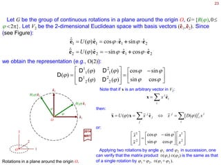
ˆ)]([ˆ)( ee D
where again g∈G. Recall that in this last equation, the index j is summed from 1 to n and
for the matrix D(g), the first index ( j) is the row-label and the second index (i) is the col-
umn-label. In the two-dimensional case of an arbitrary rotation ϕ on a plane, we get:







===
===
==
∑
∑
∑
=
=
=
2
2
21
1
2
2
1
222
2
2
11
1
1
2
1
1112
1 ˆ)(ˆ)(ˆ)]([ˆ)(ˆ
ˆ)(ˆ)(ˆ)]([ˆ)(ˆ
ˆ)]([ˆ)(
eeeee
eeeee
ee
ϕϕϕϕ
ϕϕϕϕ
ϕϕ
DDD
DDD
D
++++
++++
j
j
j
j
j
j
j
j
j
ii
U
U
U

25. 25
)()()()()()( 2121 gggggggg DDDDDD =⇔=
2017
MRT
Let us examine how the basic property of the representation operators (i.e., U(g)U(g)=
U(gg)), can be expressed in terms of the { D(g), g∈G} matrices. Apply the operators on
both sides of U(g1)U(g2)=U(g1g2) with:
∑∑∑ ==
= k j
k
j
i
k
j
n
j
j
j
ii ggggUgUgU eee ˆ)]([)]([ˆ)]([)(]ˆ)()[( 21
1
2121 DDD
Since |êi〉 form a basis, we conclude that:
where matrix multiplication is implied. So, since D(G)={ D(g), g∈G} satisfy the same
algebra as U(G), the group of matrices D(G) forms a matrix representation of G.
∑=
=
n
j
j
j
ii ggU
1
22 ˆ)]([ˆ)( ee D
we get:
∑=
k
k
k
ii ggggU ee ˆ)]([ˆ)( 2121 D
)()()( 2121 ggUgUgU =
to the basis vectors, and we obtain:
and since, in this case:

26. ê1 = R(ϕ)ê1
ê1
ê2
ê2 = R(ϕ)ê2
ϕ
O
1
2
3
O
ϕ
Rotations in a plane around the origin O.
2017
MRT
Note that if x is an arbitrary vector in V2:
2
2
1
1
2
1
ˆˆˆ eeex xxx
i
i
i
+== ∑=
21222111 ˆcosˆsinˆ)(ˆˆsinˆcosˆ)(ˆ eeeeeeee ⋅⋅−==⋅⋅== ϕϕϕϕϕϕ ++++++++ UU and
Let G be the group of continuous rotations in a plane around the origin O, G={R(ϕ),0≤
ϕ <2π}. Let V2 be the two-dimensional Euclidean space with basis vectors {ê1,ê2}. Since
(see Figure):
for {ê1,ê2}, we obtain the representation (e.g., for a plane 2D Orthogonal group O(2)):*





 −
=








≡=
ϕϕ
ϕϕ
ϕϕ
ϕϕ
ϕϕ
cossin
sincos
)()(
)()(
)]([)( 2
2
1
2
2
1
1
1
DD
DD
DD j
i
then:
∑∑ ==
=⇔==
2
1
2
1
)]([ˆ)(
i
ij
i
j
j
j
j
xxxU ϕϕ Dexx
or:













 −
=








2
1
2
1
cossin
sincos
x
x
x
x
ϕϕ
ϕϕ
Applying two rotations by angle ϕ1 and ϕ2 in succession, one
can verify that the matrix product D(ϕ1) D(ϕ2) is the same as
that of a single rotation by ϕ1 +ϕ2, D(ϕ1 +ϕ2 ).
26
* The signs of sinϕ might appear to be backwards, but they are not. If you go back to the
equation on Slide 17 and look at yj=Σi Aj
i xi, you will see the matrix elements are [ D(ϕ)]j
i .

27. 27
)ˆˆ(
2
1
ˆ 21 eee i±=± m
2017
MRT
A representation U(G) on V is irreducible if there is no non-trivial subspace in V with
respect to U(G). Otherwise, the representation is reducible (i.e., broken down further).
The one-dimensional subspace spanned by ê1 (or ê2) is not invariant under the group
R(2). However, if we form the following linear combination of (complex) vectors:
Under the action of U(ϕ), the unit vector ê+ =−(1/√2)(ê1+iê2) transform to:






−=
−−−=
+−−−=





−=
=
−
++
)ˆˆ(
2
1
e
)]sin(cosˆ)sin(cosˆ[
2
1
)]cosˆsinˆ()sinˆcosˆ[(
2
1
)ˆˆ(
2
1
)(
ˆ)(ˆ
21
21
212121
ee
ee
eeeeee
ee
i
iii
iiU
U
i
−−−−
−−−−
−−−−−−−−
ϕ
ϕϕϕϕ
ϕϕϕϕϕ
ϕ
since exp(±iϕ)=cosϕ ±isinϕ. Collecting, we get:
+
−
+ = ee ˆeˆ ϕi
In similar fashion, we obtain:
−− = ee ˆeˆ)( ϕ
ϕ i
U

28. 28
2017
MRT
So, it was straightforward to show that (Exercise):
−−+
−
+ == eeee ˆeˆ)(ˆeˆ)( ϕϕ
ϕϕ ii
UU and
Operating on any vector with a unitary operator U(ϕ) is the same as multiplying it by the
phase exp(miϕ)! Therefore, the one-dimensional spaces spanned by ê± are individually
invariant under the rotation group R(2). The two-dimensional representation given by:





 −
=
ϕϕ
ϕϕ
ϕ
cossin
sincos
)(D
can be simplified if we make a change of basis to the eigenvectors ê±. With respect to
the new basis:








=
−
ϕ
ϕ
ϕ i
i
e0
0e
)(D
The D(ϕ) matrices can be obtained from the D(ϕ) matrices by a similarity transformation
S, which is just the transformation from the original basis {ê1,ê2} to the new basis {ê+,ê−}
given by ê± =−(1/√2)(±ê1 +iê2) using:
SASASASA ee ˆ
11
ˆ
−−
=⇔= ±±±±±±±±
ee ˆ
1
ˆ xSxxSx −
=⇔= ±±±±±±±±
and:
obtained earlier (in matrix form for u=ê±).ˆ

29. 29
∑=≡
g
ggSS yxyxyx )()(),( DD
2017
MRT
If the group representation space is an inner product space, and if the operators U(G)
are unitary for all g∈G, then the representation U(G) is said to be a unitary
representation.
Every representation D(G) of a finite group on a inner product space is equivalent to a
unitary representation. That is, we need to find a non-singular operator S such that:
)()( 1
gUSgS =−
D
is unitary for all g∈G. S can be chosen to be one of those operators which satisfy the
following equation:
for all x,y∈V. The existence of S is established by noting that:
1. (x,y) satisfies the axioms (i.e., a premise or starting point of reasoning) of the
definition for a new scalar product; and
2. S represents the transformation from a basis orthonormal with respect to the scalar
product 〈 | 〉 to another basis orthonormal with respect to the new scalar product ( , ).
yxyxyx
yxyxyx
===
==
−−−−
−−−−
∑
∑
),()()(
)()()()()()()()(
1111
1111
SSSgSg
SggSggSgSSgSgUgU
g
g
DD
DDDDDD
To show that U(g) is unitary for such a choice of S, note that:

30. 30
211 ˆsinˆcosˆ)( eee ϕϕϕ +=R
2017
MRT
Continuous groups consists of group elements which are labelled by one or more
continuous variables, say (a1,a2,…,ar), where each variable has a well-defined range.
The mathematical theory of continuous groups is usually called the theory of Lie groups.
Roughly speaking, a Lie group is an infinite group whose elements can be represented
smoothly and analytically.
Rotation Group SO(2)
Consider a system symmetric under rotations in a plane, around a fixed point O. Adopt
a Cartesian coordinate frame on the plane with ê1 and ê2 as the orthonormal basis
vectors (see previous Figure). Denoting the rotation through angle ϕ by R(ϕ), we obtain
by elementary geometry:
or equivalently:
2
2
1
1
2
1
ˆ)]([ˆ)]([ˆ)]([ˆ)( eeee ii
j
j
j
ii RRRR ϕϕϕϕ +== ∑=
with the matrix [R(ϕ)]j
i given by:





 −
=
ϕϕ
ϕϕ
ϕ
cossin
sincos
)(R
212 ˆcosˆsinˆ)( eee ϕϕϕ +−=R
and:

31. 31
∑∑∑ ==≡→
i j
ij
ij
i
i
i RxRR xeexxx )]([ˆˆ)()( ϕϕϕ
2017
MRT
Let x be an arbitrary vector in the plane with components [x1,x2] with respect to the
basis {êi} (i.e., x=Σi xiêi ). Then x transforms under rotation R(ϕ) according to:
Since x=Σj x jêj , we obtain:
∑=
i
ij
i
j
xRx )]([ ϕ
Geometrically, it is obvious that the length of vectors remains invariant under rotations
(i.e., |x|2 =Σi xi xi =|x|2 =Σi xi xi). Using this last equation, we obtain the condition on the
rotational matrices:
1≡)()( ϕϕ T
RR
where RT denotes the transpose of R, and 1 is the trivial element (i.e., unit matrix). Real
matrices satisfying this last trivial condition are called orthogonal matrices.
This last equation also implies that [detR(ϕ)]2 =1 or detR(ϕ)=±1. The explicit formula
for R(ϕ) indicates that we must impose the more restrictive condition:
1)(det =ϕR
for all ϕ. Matrices satisfying this determinant condition are said to be special. Hence
these rotation matrices are special orthogonal matrices of rank 2; they are
designated as SO(2) matrices.

32. 32
)()()( 1212 ϕϕϕϕ += RRR
2017
MRT
Two rotation operations can be applied in succession, resulting in an equivalent single
rotation. Geometrically, it is obvious that the law of composition (or multiplication) is:
with the understanding that if ϕ1 +ϕ2 goes outside the range [0,2π], we have:
)π2()( ±= ϕϕ RR
So, with the law of multiplication, and with the definitions that R(ϕ =0)≡1 and R(ϕ)−1 =
R(−ϕ)=R(2π−ϕ), the two-dimensional rotation {R(ϕ)} form a group called the R2 or
SO(2) group. Note that R(ϕ2)R(ϕ1)=R(ϕ2+ϕ1) above implies R(ϕ1)R(ϕ2)=R(ϕ2)R(ϕ1) for
all ϕ1,ϕ2. Thus, the group SO(2) is Abelian.
Now, consider an infinitesimal SO(2) rotation by an angle dϕ. Differentiability of R(ϕ) in
requires that R(dϕ) differs from R(0)≡1 by only a quantity of order dϕ which we define by
the relation:
JdidR ϕϕ −= 1)(
where the (complex) factor −i is included by convention and for later convenience (e.g.,
to make things Hermetian by definition!) Furthermore, the quantity J is independent of
the rotation angle dϕ.












−





=
2221
1211
0
0
10
01
)(
JJ
JJ
d
d
idR
ϕ
ϕ
ϕ
In matrix form, R(dϕ) is represented by:
where the 4 components of J needs to be found.

33. 33
ϕ
ϕ
ϕϕϕϕ
ϕϕϕϕϕϕϕϕϕ
d
Rd
dRdR
JRidRJdiRdRRdR
)(
)()(
])([)())(()()()(
+=+
−+=⋅−==+ 11
2017
MRT
Next, consider the rotation R(ϕ +dϕ), which can be evaluated in two ways:
Comparing the two equations, we get the differential equation:
0)(
)(
)(
)(
=+⇒−= ϕ
ϕ
ϕ
ϕ
ϕ
ϕ
RJi
d
Rd
RJi
d
Rd
We have, of course, also the boundary condition R(0)≡1.
Ji
R ϕ
ϕ −
= e)(
J is called the generator of the group.
The solution to this last first-order differential equation (in constant coefficients) is
therefore unique for all two-dimensional rotations can be expressed in terms of the
operator J as:
ϕ
ϕ
ϕ
dJi
R
Rd
−=
)(
)(
When integration is done we get:
ϕϕ JiCR −=+)(ln
and by exponentiating and using R(0)≡1 to find that C=0 and then we get the solution:

34. 34
2017
MRT
Let us turn from this abstract discussion to the explicit representation of R(dϕ) to first
order:





 −
=⇔




 −
=
1
1
)(
cossin
sincos
)(
ϕ
ϕ
ϕ
ϕϕ
ϕϕ
ϕ
d
d
dRR
Comparing with the R(dϕ)=1−idϕ J matrix above, we find that the rotation generator is:





 −
=




 −
=
01
10
0
0
i
i
i
J
Thus J is a traceless Hermitian matrix with off-diagonal antisymmetric components.





 −
+





=




 −
−





=
−=








+−−








+−=+








−−−−=
×
−
0sin
sin0
cos0
0cos
sin
0
0
cos
10
01
sincos
!3!2
1
!3!2
e
22
3232
ϕ
ϕ
ϕ
ϕ
ϕϕ
ϕϕ
ϕ
ϕ
ϕϕϕ
ϕϕ
i
i
i
JiI
JiJiJiJi
KKK 111
since i2 =−1 which reduces to:
Ji
R ϕ
ϕϕ
ϕϕ
ϕ −
=




 −
= e
cossin
sincos
)(
It is easy to show (Exercise) that J 2 =1, J3 =J, … &c. Therefore:

35. 35
2017
MRT
Consider any representation of SO(2) defined on a finite dimensional vector space V. Let
U(ϕ) be the operator on V which corresponds to R(ϕ). Then, according to R(ϕ2)R(ϕ1)=
R(ϕ2 +ϕ1), we must have U(ϕ2)U(ϕ1)=U(ϕ2 +ϕ1) =U(ϕ1)U(ϕ2) with the same
understanding that U(ϕ)=U(ϕ ±2π). For an infinitesimal transformation, we can again
define an operator corresponding to the generator J in R(dϕ)=1 − idϕ J. We use the
same letter J to denote this operator:
Irreducible Representation of SO(2)
JdidU ϕϕ −= 1)(
Repeating the arguments of the last chapter, we obtain:
Ji
U ϕ
ϕ −
= e)(
which is now an operator equation on V. If U(ϕ) is to be unitary for all ϕ, J must be
Hermitian.
Since SO(2) is an Abelian group, all its irreducible representations are one-
dimensional. This means that given any vector |α〉 in a minimal invariant subspace under
SO(2) we must have J|α〉=α|α〉 and U(ϕ)|α〉=exp(−iϕα)|α〉 where the label α is a real
number chosen to coincide with the eigenvalue of the Hermitian operator J. In order to
satisfy the global constant U(ϕ)=U(ϕ ±2π), a restriction must be placed on the
eigenvalue α. Indeed, we must have exp(+2πiα)≡1, which implies that α is an integer.
We denote this integer by m, and the corresponding representation by Um:
mmUmmmJ mim ϕ
ϕ −
== e)(and

36. 36
oo)( xxxxT +=
2017
MRT
Rotations in the two-dimensional plane (e.g., by an angle ϕ) can be interpreted as
translations of the unit circle (e.g., by the arc length ϕ). This fact accounts for the
similarity in the form of the irreducible representation function (i.e., Un(ϕ)=exp(−inϕ)) in
comparison to the case of discrete translation on a one-dimensional lattice of spacing b
which is given by tk(n)=exp(−inkb) with k the wave vector. We now extend the
investigation to the equally important and basic continuous translation group in one
dimension, which we shall refer to as T1.
Continuous Translational Group
Let the coordinate axis of the one-dimensional space be labelled x (the generalization
to the three dimensional case is trivially done for x or r). An arbitrary element of the
group T1 corresponding to translation by a distance x will be denoted by T(x). Consider
states |xo〉 of a particle localized at the position xo. The action of T(x) on |x〉 is:
T(x) must have the following properties... First group multiplication:
)()()( 2121 xxTxTxT +=
And, finally, an inverse:
These are just the properties required for {T(x), −∞< x<∞} to form a group.
)()( 1
xTxT −=−
1≡)0(T
Then an initial condition:

37. 37
PxdidxT −= 1)(
2017
MRT
For an infinitesimal displacement denoted by dx, we have:
which defines the (displacement-independent) generator of translation P. Next, we write
T(x+dx) in two different ways (like before for R(ϕ)):
xd
xTd
xdxTxdxT
PxTixdxTPxdixTxdTxTxdxT
)(
)()(
])([)())(()()()(
+=+
−+=−==+ 11
Comparing the two equations, we get the differential equation dT(x)/dx=−iPT(x) and
considering the boundary condition T(0)≡1, this differential equation yields the unique
solution:
xPi
xT −
= e)(
With T(x) written in this form, all the required group properties are satisfied. This
derivation is identical to that given for the rotation group SO(2). The only difference is
that the parameter x in T(x) is no longer restricted to a finite range as for ϕ in R(ϕ).
As before, all irreducible representations of the translation group are one-dimensional.
For unitary representations, the generator P corresponds to a Hermitian operator with
real eigenvalues, which we shall denote by p. For the representation T(x)→Up(x), we
obtain:
ppxUpppP xpip −
== e)(and

38. 38
oo)( ϕϕϕϕ +=U
2017
MRT
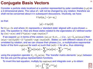
Consider a particle state localized at a position represented by polar coordinates [r,ϕ] on
a two-dimensional plane. The value of r will not be changed by any rotation; therefore
we shall not be concerned about it in subsequent discussions. Intuitively, we have:
Conjugate Basis Vectors
so that:
0)(ϕϕ U=
for 0≤ϕ <2π and where |0〉 represents a standard state aligned with a pre-chosen x-axis.
The question is: How are these states related to the eigenstates of J defined earlier by
J|m〉=m|m〉 and Um(ϕ)|m〉=exp(−imϕ)|m〉?
If we expand |ϕ 〉 in terms of the vectors {|m〉,m=0,±1,…} (i.e., |ϕ 〉=Σm|m〉〈m|ϕ〉) then
〈m|ϕ〉=〈m|U(ϕ)|0〉=〈U †(ϕ)m|0〉=exp(−imϕ)〈m|0〉. States |m〉 with different values of m are
unrelated by rotation, and we can choose their phases (i.e., a multiplicative exponential
factor of the form exp(iαm) for each m) such that 〈m|0〉=1 for all m, thus obtaining:
∑∑ ∑ −
±=
===
m
mi
m m
mmmmm ϕ
ϕϕϕ e
,1,0 K
using the projection operator Em =Σm=0,±1,…|m〉〈m|. The transfer matrix elements 〈m|ϕ〉
between the two are just the group representation functions.
∫=
π2
0
e
π2
ϕ
ϕ ϕmid
m
To invert this last equation, multiply by exp(imϕ) and integrate over ϕ to obtain:

39. 39
∫∫ ∑∑ ∫∑ =








===
π2
0
π2
0
π2
0
)(
π2
e
π2
e
π2
ϕϕψ
ϕ
ϕψ
ϕ
ϕ
ϕ
ψψψ ϕϕ ddd
m
m
m
mi
m
mi
m
m
m
2017
MRT
An arbitrary state |ψ 〉 in the vector space can be expressed in either of the two bases:
The wave functions ψm=〈m|ψ 〉 and ψ(ϕ) are related by (with 〈ϕ |m〉=〈m|ϕ〉*=exp(imϕ)):
∑∑ ====
m
m
mi
m
mm ψψϕψϕψϕϕψ ϕ
e)( 1
and:
∫
−
=
π2
0
e)(
π2
ϕ
ϕψ
ϕ
ψ mi
m
d
Let us examine the action of the operator J on the states |ϕ 〉. From |ϕ 〉=Σmexp(−imϕ)|m〉
we obtain:
ϕ
ϕ
ϕ ϕϕϕ
d
d
immmJmJJ
m
mi
m
mi
m
mi
==== ∑∑∑ −−−
eee
since J|m〉=m|m〉. For an arbitrary state, we have:
ϕ
ϕψ
ψϕ
ϕ
ψϕψϕ
d
d
id
d
i
JJ
)(11
===
J is the angular momentum operator (measured in units of h).
The above purely group-theoretical derivation underlines the general, geometrical
origin of these results.

40. 40
∫∫
∞
∞−
∞
∞−
−
== xxdpp
pd
x xpixpi
ee
π2
and
2017
MRT
The above discussion can be repeated for the continuous translation group. The
localized states |x〉 (i.e., T(x)|x〉=|x+xo〉) and the translationally covariant states |p〉 (i.e.,
P|p〉=p|p〉) are related by:
where the normalization of the states is chosen as 〈x|x〉=δ (x−x) and 〈 p|p〉=2πδ (p−p).
Now, the transfer matrix elements are the group representation functions (i.e., Up(x)|p〉=
exp(−ipx)|p〉):
xpi
xp −
= e
As before, if:
∫∫
∞
∞−
∞
∞−
== pp
pd
xxxd )(
π2
)( ψψψ
then:
∫∫
∞
∞−
−
∞
∞−
== )(e)()(e
π2
)( xxdpp
pd
x xpixpi
ψψψψ and
xd
xd
iPPx x
)(ψ
ψψ −==
and:
Thus, the generator P can be identified with the linear momentum operator in
quantum mechanical systems.

41. 41
apixpiapixpiaxpia xxxxx
axx eeee)()( )(
===+→ ++
ψψ
2017
MRT
Note that in the (e.g., one-dimensional) position representation, x, the matrix elements
(wavefunction) of a momentum eigenstate are:
xpi
p
x
xpx e)( ==ψ
The wavefunction,ψ (x), shifted by a constant finite translation a is:
Now the momentum operator px is the thing which, acting on the momentum eigenstate,
returns the value of the momentum in these states. This has been learned as −id/dx.
For our momentum eigenstate,ψ (x), if we spatially shift it by an infinitesimal amount ε,
it becomes:
xpi
x
xpipipixpixpi xxxxxx
pixx e)1(eeee)()( )(
L++====+→ ++
εεψψ εεεε
that is, the shift modifies it by an expansion in its momentum value. But now, if we Taylor
expand ψ (x+ε), we get:
LL +





−+=++=+ )()()()()( x
xd
d
iixx
xd
d
xx ψεψψεψεψ
So, this is consistent since the infinitesimal spatial shift operator px =−id/dx is precisely
the operator which is pulling out the momentum eigenvalue.
Of course, the developments above can be generalized to the three-dimensional
case.

42. 42
∑=
=→
3
1
ˆˆˆ
j
j
j
iii eee RR
2017
MRT
The groups discussed so far have all been Abelian. The group multiplication rules are
very simple and the representation functions share universal features. We now study the
best known and most useful non-Abelian continuous group – SO(3), the group of ortho-
gonal (i.e., the O) rotations in three dimensions (i.e., the (3)) with unit determinant (i.e.,
special, S). The SO(3) group consists of all continuous linear transformations in three-
dimensional Euclidean space which leave the length of coordinate vectors invariant.
Description of the Group SO(3)
Consider a Cartesian coordinate frame specified by the orthonormal vectors êi, i=1,2,
3. Under a rotation:
where Rj
i are elements of 3×3 rotational matrices. Let x be an arbitrary vector, x=Σi xiêi,
then x→x under rotation R such that:
∑=≡
j
ji
j
ii
xxx R
The requirement that |x|=|x|, or Σi xi xi =Σi xi xi, yields RRT =RTR≡1 for all rotational
matrices. Real matrices satisfying this condition have determinants equal to ±1. Since
all physical rotations can be reached continuously from the identity transformation
(i.e., zero angle of rotation), and since the determinant for the latter is +1, it follows
that all rotation matrices must have determinant +1. Thus, in addition to R RT =RTR=
1, the matrices R are restricted by the condition det R=1.

43. 43
i
j
j
j
i
k
k
k
i
kj
k
j
i
k
j
j
j
j
ii eeeeee ˆˆ][ˆ][ˆ][][ˆ][ˆ 3312121212 RRRRRRRRRR ===== ∑∑∑∑
Consider performing rotation R1, followed by rotation R2. The effect on the coordinate
vectors can be expressed as follows:
Therefore, the net result is equivalent to a single rotation R3:
312 RRR =
where matrix multiplication on the right-hand side is understood. The conclusions are:
1. the product of two SO(3) matrices is again an SO(3) matrix;
2. the identity matrix is an SO(3) matrix; and
3. each SO(3) matrix has an inverse–the rotation matrices for a group–the SO(3) group.
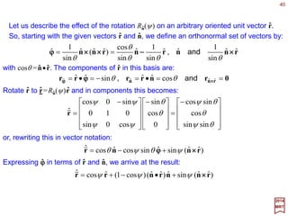
The SO(3) group manifold in the angle-axis
parameterization.
2017
MRT
x
y
z
ψ
θ
ϕ
Any rotation can be designated by Rn(ψ ) where the unit vector
n specifies the direction of the axis of rotation and ψ denotes the
angle of rotation around that axis. Since the unit vector n, in turn,
is determined by the two angles – say the polar and the
azimuthal angles [θ,ϕ] of its direction – we see that R is
characterized by the three parameters [ψ ,θ,ϕ] where 0≤ ψ ≤π, 0
≤θ ≤π, and 0 ≤ϕ <2π.
ˆ
ˆ
ˆ
There is a redundancy in this parameterization R−n(π) = Rn(π).
The structure of the group parameter space can be visualized by
associating each rotation with a three dimensional vector c= ψn
pointing in the direction n with magnitude equal to ψ (see Figure).
Note that the tips of these vectors fill a three-dimensional sphere
of radius π.
ˆ
ˆ
ˆ ˆ
ˆn

44. Let us describe the effect of the rotation RRRRn(ψ) on an arbitrary oriented unit vector r.ˆ
rnnrnrnn ˆˆ
sin
1
ˆˆ
sin
1
ˆ
sin
cos
)ˆˆ(ˆ
sin
1
ˆ ××××−−−−××××××××ϕϕϕϕ
θθθ
θ
θ
and,==
with cosθ =n•r. The components of r in this basis are:ˆ ˆ ˆ
0rnrrrr rnn ==•=−=•= ˆˆˆˆ cosˆˆsinˆˆ ××××ϕϕϕϕ ϕϕϕϕ and, θθ
Rotate r to r= Rn(ψ)r and in components this becomes:









−
=









−









 −
=
θψ
θ
θψ
θ
θ
ψψ
ψψ
sinsin
cos
sincos
0
cos
sin
cos0sin
010
sin0cos
ˆr
or, rewriting this in vector notation:
ˆˆ ˆ ˆ
)ˆˆ(sinˆsincosˆcosˆ rnnr ××××ϕϕϕϕ ψθψθ +−=
Expressing ϕϕϕϕ in terms of r and n, we arrive at the result:ˆ ˆ ˆ
)ˆˆ(sinˆ)ˆˆ()cos1(ˆcosˆ rnnrnrr ××××ψψψ +•−+=
44
2017
MRT
So, starting with the given vectors r and n, we define an orthonormal set of vectors by:
ˆ
ˆ ˆ

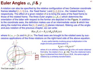
45. 1
x
x
2
3, z
α
y, y, n
β
α
β
Z, z
γ
γ
Y
ˆ
X
The Euler angles α, β, and γ.
2017
MRT
A very useful identity involving group multiplication in the
angle-and-axis parameterization is:
1
ˆ )()( −
= RRRR ψψn
A rotation can also be specified by the relative configuration of two Cartesian coordinate
frames labelled [1,2,3] (i.e., the rotated frame or body frame) and [X,Y,Z] (i.e., the fixed
frame or inertial frame), respectively. The effect of a given rotation R is to bring the axes
of the fixed frame to those of the rotated frame. The three Euler angles [α,β,γ ] which
determine the orientation of the latter with respect to the former are depicted in the
Figure. In addition to the coordinate axes, the definition makes use of an interme-diate
vector n which lies along the nodal line where the [1,2] and [X,Y] planes intersect.
Making use of the angle-and-axis notation of the previous chapter, we can write:
Euler Angles α, β & γ
where 0≤α, γ <2π and 0≤β ≤π. The fixed axes are brought to the rotated axes by suc-
cessive applications of the three rotations on the right-hand side of the above equation.
where R is an arbitrary rotation and n is the unit vector obtained
from n by the rotation R (i.e., n= Rn). Thus the rotational matrix
Rn(ψ ) is obtained from that of Rn(ψ ) (N.B., the same angle of
rotation) by a similarity transformation.
ˆ
ˆ ˆ ˆ
ˆ ˆ
ˆ
45
R(α,β,γ )=RZ(γ )Rn(β)R3(α)
ˆn
ˆ

46. 46
)()()()()()()()( 1
323ˆ
1
ˆ3ˆ αβαββγβγ −−
== RRRRRRRRZ nnn and
2017
MRT
Using the similarity transformation above, we can re-express R(α,β,γ) in terms of
rotations around a fixed axis:
Substituting the first of the identities in R(α,β,γ)=RZ(γ)Rn(β)R3(α) above, we obtain the
rotation Rn(β)⋅⋅⋅⋅R3(γ +α) for the right-hand side. Making use of the second identity above,
we obtain:
)()()(),,( 323 γβαγβα RRRR =
Thus, in terms of the Euler angles, every rotation can be decomposed into a product of
simple rotations around the fixed axes ê2 and ê3 (i.e., 2 and 3).
ˆ
ˆ
In view of the last equation, it is necessary to obtain expressions for R2(ψ) and R3(ψ).
Using the original definition (i.e., êi =ΣjRj
i êj), we can show that (Exercise):










−
=









 −
=
ψψ
ψψ
ψψψ
ψψ
ψ
cos0sin
010
sin0cos
)(
100
0cossin
0sincos
)( 23 RR and
and, for completeness:










−=
ψψ
ψψψ
cossin0
sincos0
001
)(1R
ˆ ˆ

47. 47
2017
MRT
Substituting these matrices into R(α,β,γ)=R3(α)R2(β)R3(γ) one can obtain a formula
for the 3×3 matrix representing a general SO(3) transformation (i.e., a 3D rotation – we
used R before). Performing the matrix multiplication, the result is:










−
+−+
−−
=
βγβγβ
βαγαγβαγαγβα
βαγαγβαγαγβα
γβα
cossinsincossin
sinsincoscossincossinsincoscoscossin
sincoscossinsincoscossinsincoscoscos
),,(R
One can also compare this expression with the angle-and-axis parameterization to
derive the relations between the variables [α,β,γ ] and [ψ,θ,ϕ] for a given rotation. The
results are:
1
2
cos
2
cos2cos
2
sin
2
tan
tan
2
π 22
−




 +






=





 +






=
−+
=
γαβ
ψ
αγ
θ
θ
γα
ϕ and,
which were obtained by:
1. using the trace condition (i.e., TrR(α,β,γ)=TrRn(ψ)); and
2. considering that n is left invariant by the rotation R(α,β,γ) (i.e., R(α,β,γ)n=Rn(ψ)n=n
with n=[cosϕ sinθ sinϕ sinθ cosθ]T)
ˆ
ˆˆ ˆ ˆˆ
ˆ

48. 48
n
n
ˆ
e)(ˆ
Ji
R ψ
ψ −
=
2017
MRT
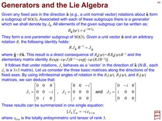
Given any fixed axis in the direction n (e.g., a unit normal vector) rotations about n form
a subgroup of SO(3). Associated with each of these subgroups there is a generator
which we shall denote by Jn. All elements of the given subgroup can be written as:
Generators and the Lie Algebra
ˆ ˆ
They form a one parameter subgroup of SO(3). Given a unit vector n and an arbitrary
rotation R, the following identity holds:
ˆ
nn ˆ
1
ˆ JRJR =−
where n=Rn. This result is a direct consequence of Rn(ψ)=RRn(ψ)R−1 and the
elementary matrix identity Rexp(−iψ J)R−1 =exp[−iψ (RJR−1)].
ˆˆ
ˆ ˆ
It follows that under rotations, Jn behaves as a vector in the direction of n (N.B., each
Jn is a 3×3 matrix). Let us consider the three basic matrices along the directions of the
fixed axes. By using infinitesimal angles of rotation in the R1(ψ), R2(ψ), and R3(ψ)
matrices, we can deduce that:
ˆ









 −
=









 −
=










−=
000
00
00
00
000
00
00
00
000
321 i
i
J
i
i
J
i
iJ and,
These results can be summarized in one single equation:
mkmk iJ l
l
ε−=][
where εklm is the totally antisymmetric unit tensor of rank 3.
ˆ

49. 49
∑=−
l
l
l
JRRJR kk
1
2017
MRT
Under rotations, the vector generator J (i.e., with components {Jk ,k=1,2,3}) behave
the same way as the coordinate vectors {êk}:
and the generator of rotations around an arbitrary direction n can be written as:ˆ
∑=
k
k
k nJJ ˆˆn
where n=Σk nk êk. This equation shows that {J1,J2,J3} form the basis for the generators of
all one-parameter Abelian subgroups of SO(3), and:
ˆ
∑−
= k
k
k nJi
R
ˆ
ˆ e)(
ψ
ψn
Similarly, we can write the Euler angle representation, R(α,β,γ)=R3(α)R2(β)R3(γ), in
terms of the generators:
323
eee),,( JiJiJi
R γβα
γβα −−−
=
Therefore, for all practical purposes, if suffices to work with the three basis-generators
{Jk} rather than the three-fold infinity group elements R(α,β,γ).
The three basis generators {Jk} satisfy the following Lie algebra:
∑=
m
m
mkk JiJJ ll ε],[
where the left-hand side is the commutator of Jk and Jl (i.e., [Jk ,Jl]=Jk Jl − Jl Jk).
ˆ

50. 50
0)](,[ ˆ =ψnRH
2017
MRT
We finish this chapter with a few more remarks:
1. It is fairly straightforward to verify that the matrices given by J1, J2, and J3 satisfy the
commutation relations specified by [Jk ,Jl]=iΣmεklm Jm, as they should;
2. If on the space of the generators {Jk} and all their linear combinations, one defines
multiplication of two elements as taking their commutator, then the resulting
mathematical system forms a linear algebra. This is the reason for using the
terminology Lie algebra of the group under consideration; and
3. In physics, the generators acquire even more significance, as they correspond to
physically measurable quantities. Thus {Jk} have the physical interpretation as
components of the vector angular momentum operator (measured in units of h). The
equation [Jk ,Jl]=iΣmεklm Jm are recognized as the commutation relations of the
quantum mechanical angular momentum operators.
We also note that if a physical system represented by a Hamiltonian H is invariant
under rotations, then:
for all n and ψ. This is equivalent to the simpler condition:
0],[ =kJH
for k=1,2,3. This implies that the physical quantities corresponding to the generators of
the symmetry group are, in addition, conserved quantities.
We see here again with the generator another prime example of the close
connection between pure mathematics and physics.
ˆ

51. 51
2
3
2
2
2
1
2
)()()( JJJ ++=•= JJJ
2017
MRT
In this chapter, we construct the irreducible representations of the Lie algebra of SO(3),
[Jk ,Jl]=iΣmεklm Jm. Due to the fact that the group parameter space is compact, we expect
that the irreducible representations are finite-dimensional, and that they are all
equivalent to unitary representations. Correspondingly, the generators will be
represented by Hermitian operators.
Irreducible Representation of SO(3)
The basis vectors of the representation space V are naturally chosen to be
eigenvectors of a set of mutually commuting generators. The generators J1, J2, and J3 do
not commute with each other. However, any single one does commute with the
composite operator:
That is:
0],[ 2
=JJk
for k=1,2,3.
J2 is an example of a Casimir operator – an operator which commutes with all
elements of a Lie group. This last equation implies that J2 commutes with all SO(3) group
transformations.
By convention, the basis vectors are chosen as eigenvectors of the commuting
operators [J 2, J3]. The remaining generators also play an important role, in the form of
raising and lowering operators:
21 JiJJ ±=±

52. 52
K,2,
2
3
,1,
2
1
,0=j
2017
MRT
Without having to prove this (c.f., Sakurai, Ch. 3), the eigenvalue j is given by:
and these are normalized such that mj= j, j−1, j−2,…. The irreducible representations of
the Lie algebra of SO(3), [Jk ,Jl]=iΣmεklm Jm, are each characterized by an angular
momentum eigenvalue j from the set of positive integers and half-integers. The
orthonormal basis vectors can be specified by the following equations:
1,)1()1(,,,,)1(, 3
2
±±−+==+= ± jjjjjjjjj mjmmjjmjJmjmmjJmjjjmjJ and,
Knowing how the generators act on the basis vectors, we can immediately derive the
matrix elements in the various irreducible representations. Let us write:
∑′
′
′=
j
j
j
m
j
m
m
j
j mjmjU ,)],,([,),,( )(
γβαγβα D
where U is the operator representing the group elements R(α,β,γ). We can deduce from
R(α,β,γ)=exp(−iα J3)exp(−iβ J2)exp(−iγ J3) that:
jj
j
jj
j
mim
m
jmim
m
j
d
γα
βγβα
−′′−′
= e)]([e)],,([ )()(
D
where:
j
Ji
j
m
m
j
mjmjd j
j
,e,)]([ 2)( β
β −′
′=
The d( j)-matrices are real orthogonal.

53. 53
2017
MRT
For j=0 (and mj=0), we get J3 =[0], J+ =[0] and J− =[0].






=





=





−
=








−
= −+
01
00
00
10
10
01
2
1
0
0
2
1
2
1
3 JJJ and,
or Jk =½σk, k=1,2,3, where σk are the Pauli matrices:






−
=




 −
=





=
10
01
0
0
01
10
321 σσσ and,
i
i
By making use of the property σk
2 =I2×2 (valid only for j=½), we can derive:
For j=½ (and mj=−½, +½), we get:






























−





=





−





== ×
−
2
cos
2
sin
2
sin
2
cos
2
sin
2
cose)( 222
2)21( 2
ββ
ββ
β
σ
β
β σβ
iId i
Hence:






























−





=
−
−−−
2222
2222
)21(
e
2
cosee
2
sine
e
2
sinee
2
cose
),,(
γαγα
γαγα
ββ
ββ
γβα
iiii
iiii
D

54. 54
2017
MRT
The next simplest case is j=1. We obtain:










−
=
100
000
001
3J
The D-matrix is given by:
jj
j
jj
j
mim
m
mim
m d
γα
βγβα
−′′−′
= e)]([e)],,([ )1()1(
D
with:


















+
−
−
−
−
+
=
2
cos1
2
sin
2
cos1
2
sin
cos
2
sin
2
cos1
2
sin
2
cos1
)()1(
βββ
β
β
β
βββ
βd










=










=










=










= −+
010
001
000
2
2
020
002
000
000
100
010
2
2
000
200
020
JJ and
as well as:

55. 55
2017
MRT
We will now review the properties of the rotational matrices D( j)(α,β,γ).
),,(),,(),,( )(1)(†)(
γβαγβαγβα −−−== − jjj
DDD
All the irreducible representations of SO(3) described so far are constructed to be
unitary. Hence the D-matrices satisfy the relation:
We can show (Exercise) that the determinant of every D-matrix is equal to 1:
1),,(det )(
=γβαj
D
For integer values of j, which we shall denote by l, the D-functions are closely related
to the spherical harmonics Ylml
are Legendre functions. Specifically:
l
l
l
l
l m
mY 0
)(
)*]0,,([
π4
12
),( ϕθϕθ D
+
=
and:
0
0
)(
00
)(
)]([)(cos)(cos)]([
!)(
!)(
)1()(cos θθθθθ l
ll
l
l
l
l
ll
l
l
l
dPPd
m
m
P mm
m =
−
+
−= and
where Pl(cosθ) is the ordinary Legendre polynomials and Plml
(cosθ) is the associated
Legendre functions.

56. 56
0)](,[ =RUH
2017
MRT
We apply the group-theoretical notions developed so far to a familiar system in quantum
mechanics – a single particle in a central potential (or, equivalently, two particles
interacting with each other in their center-of-mass frame). The fact that the potential
functions V(r) depends on the magnitude r of the coordinate vector x is a manifestation
of the rotational symmetry of the system. The mathematical statement of this symmetry
principle is:
Particle in a Central Field
where H is the Hamiltonian that governs the dynamics of the system, and U(R) is the
unitary operator on the state-vector space representing the rotation R (i.e., R∈SO(3)). It
follows from the commutator above that:
0],[ =iJH
for i=1,2,3.
The quantum mechanical states of this system are most naturally chosen as
eigenstates of the commuting operators {H,J 2,J3} and will be denoted by |E,l,ml〉. They
satisfy:
lllllll llllllll mEmmEJmEmEJmEEmEH ,,,,,,)1(,,,,,, 3
2
=+== and,
where l is an integer and ml=−l,…,+l. The Schrödinger wave function of these states is:
ll ll
mEmE ,,)( xx =ψ
where |x〉 is an eigenstate of the position operator X.

57. 57
0,0,eeˆ)0,,(,, 23
rrUr JiJi θϕ
θϕϕθ −−
== z
2017
MRT
We shall use spherical coordinates [r,θ,ϕ] for the coordinate vector x, and fix the
relative phase of the vector |x〉≡|r,θ,ϕ〉 by:
Note that we have chosen to define all states in terms of a standard reference state |rz〉
≡|r,0,0〉 that represents a state localized on the z-axis at a distance r away from the
origin. For a structureless particle, of the type that is tacitly assumed here, such a state
must be invariant under a rotation around the z-axis. We have:
ˆ
0,0,0,0,e 3
rrJi
=− ψ
hence J3|r,0,0〉=0. Combining the above equations, we obtain:
∑′
′
′==
l
l
ll l
l
ll ll
m
m
mmE mErmEUr ,,0,0,])0,,([,,)0,,(0,0,)( †)(†
θϕθϕψ Dx
Because of exp(−iψ J3)|r,0,0〉=|r,0,0〉 above, we must have 〈r,0,0|E,l,m′l〉=δm′l 0ψEl (r)
which implies:
)(~)*]0,,([)( 0
)(
rE
m
mE l
l
l
l
l
ψθϕψ D=x
Making use of Ylml
(θ,ϕ)=√[(2l+1)/4π] [ D(l)(ϕ,θ,0)*]ml
0, we arrive at the result:
),()(),,( ϕθψϕθψ ll lll mEmE Yrr =
where ψEl (r)=√[4π/(2l+1)]ψEl (r). This last equation gives the familiar decomposition
of ψ (x) into the general angular factor Ylml
(θ,ϕ) (spherical symmetry) and a radial
wave function ψEl (r) which depends on the yet-unspecified potential function V(r).
~
~

58. 58
m
p
E
2
2
=
2017
MRT
If the potential function V(r) vanishes faster than 1/r at large distances, the asymptotic
states far away from the origin are close to free-particle plane wave states, these are
eigenstates of the vector momentum operator P. If we denote the magnitude of the
momentum by p and specify its direction by p(θ,ϕ), then:ˆ
and:
zp ˆ)0,,(,, pUp θϕϕθ ==
where, again, we have picked the standard reference state to be along the z-axis. These
plane-wave states can be related to the angular momentum states by making use of the
projector technique (e.g., using the projection operator Ei =Σi|êi〉〈êi|) to show that:
ϕθϕθϕθθϕθϕ ,,),(,,)*]0,,([)(cos
π4
12
,,
π2
0
1
1
0
)(
pYdpddmp m
m
∫∫ ∫ Ω=
+
=
+
− l
l
l
l
l
l
l D
where dΩ=dϕ d(cosθ). The inverse to this last relation is:
∑ ∗
=
l
l ll l
m
m mpYp ,,),(,, ϕθϕθ

59. 59
0,0,,, pSpS if ϕθ=pp
2017
MRT
Consider the scattering of a article in the (central) potential field V(r). Let the
momentum of the initial asymptotic state be along the z-axis (i.e., pi =[p,θi =0,ϕi =0]), and
that of the final state be along the direction [θi ,ϕi ] (i.e., pf =[p,θi ,ϕi ]). Then the
scattering amplitude can be written as:
where the scattering operator S depends on the Hamiltonian. The only property of S
which we shall use is that it be rotationally invariant. This means, when applied to a state
of definite angular momentum, S will leave the quantum numbers (l,ml) unchanged:
)(,,,, pSmpSmp mm lllll ll
ll ′′=′′ δδ
Let us now apply |p,θ,ϕ〉=Σml
Ylml
*(θ,ϕ )|p,l,ml〉 and 〈pf |S|pi〉=〈p,θ,ϕ|S|p,0,0〉 above,
making use of our last equation, we obtain:
)(cos)(
π4
12
),(0,,,, 0 θϕθ ll
ll l
lll
l
ll
l
l
PESYpSmpYS
m
mif ∑∑∑
+
=′=
′
∗
′pp
This is the famous partial wave expansion of the scattering amplitude. We see that its
validity is intimately tied to the underlying spherical symmetry, being quite independent
of the detailed interactions. All the dynamics resides in the yet unspecified partial-wave
amplitude Sl(E ).

60. 60
xxx RRU ==)(
2017
MRT
So far, we have concentrated on transformation properties of state vectors under
symmetry operations. In physical applications, it is useful to consider also transformation
properties of wave functions and operators under symmetry operations.
Transformation Law for Wave Functions
As our starting point, consider the basic relation:
with xi =ΣjRi
j xj. x and x are coordinate space three-vectors while |x〉 and |x〉 are
localized states at x and x, respectively, and R∈SO(3) is a rotation. Let |ψ〉 be an
arbitrary state vector, then:
∫∫
∞
∞−
∞
∞−
== xxxxxx )(33
ψψψ dd
where ψ (x)=〈x|ψ 〉 is the c-number (i.e., complex number) wave function in the
coordinate representation. We ask: How does ψ (x) transform under a rotation R; or,
more specifically, if:
∫
∞
∞−
== xxx )()( 3
ψψψ dRU
then how is ψ (x) related to ψ (x)? When we apply the rotation to both sides of the
arbitrary state |ψ〉=∫±∞ d3xψ (x)|x〉, we obtain:
∫∫∫∫
∞
∞−
−
∞
∞−
−
∞
∞−
∞
∞−
==== xxxxxxxxxxxx )()()()()()( 131333
RdRddRUdRU ψψψψψ
where the second equality follows from U(R)|x〉=|x〉, the third results from a change
of integration variable x→x and the last is due to renaming this dummy variable.

61. 61
xpxp
xx •−•−−
===
−
RiRi
p R ee)()(
1
1
ψψ
2017
MRT
As an example, let |ψ〉=|p〉 be a plane-wave state (e.g., |p〉=|p,θ,ϕ 〉=U(ϕ,θ,0)|pz〉)
then ψ p(x)=exp(ip•x) (c.f., 〈p|x〉=exp(−ipx)). Applying our transformation under
rotations:
ˆ
This is just what we expect, as:
)()()( xpxpxpxx pRRU ψψ ====
where p=Rp.
As another example, let |ψ〉=|E,l,ml〉. According to ψElml
(r,θ,ϕ)=ψEl (r)Ylml
(θ,ϕ),
where Ylml
(θ,ϕ) are the spherical harmonics for the polar θ and azimuthal ϕ angles of
the unit vector x. On the other hand, |ψ〉=U(R) Σm′l
D(l)[R]m′l
ml
|E,l,m′l〉, hence:ˆ
∑′
′
′
=
l
l
l
l
l
l
l
m
m
m
mE YRrx )ˆ(][)()( )(
xDψψ
Applying the transformation under rotations, we get:
∑′
′
′−
=
l
l
l
ll l
l
l
m
m
m
mm YRRY )ˆ(][)ˆ( )(1
xx D
which is a well known property of the spherical harmonics known as the transformation
law of the spherical harmonics:
∑′
′
′
=
l
l
l
ll l
l
l
m
m
m
mm YY ),()],,([),( )(
ψξγβαϕθ D

62. 62
)()()( 1
xxx −
=→ Rψψψ
2017
MRT
So, the wave function of an arbitrary state transform under rotations as:
Let us generalize this wave functions that also carry a discrete index (e.g., σ ). For
concreteness’ sake, let us consider the case of coordinate space wave functions, this
time spin-½ objects – these are the Pauli spinor wave functions. The basis vectors are
chosen to be {|x,σ〉,σ =±½}, and they transform as:
∑=
λ
λ
σ λσ ,][,)( )21(
xx RRRU D
where D(1/2)[R] is the angular momentum ½ rotation matrix. An arbitrary state of such a
spin-½ object can be written as:
∑∫
∞
∞−
=
σ
σ
σψ ,)(3
xxxdΨΨΨΨ
where ψ σ (x) is the two-component Pauli wave function of |ΨΨΨΨ〉.

63. 63
2017
MRT
How does the Pauli wave function ψ σ (x) transform under rotation? Well, we have:
∑∫
∑∫
∑∫ ∑
∑∫
∞
∞−
∞
∞−
−
∞
∞−
∞
∞−
=
=
=
==
λ
λ
λσ
σλ
σ
σ λ
λ
σ
σ
σ
σ
λψ
λψ
λψ
σψ
,)(
,)(][
,][)(
,)()()(
3
1)21(3
)21(3
3
xxx
xxx
xxx
xxx
d
RRd
RRd
RUdRU
D
D
ΨΨΨΨΨΨΨΨ
Hence, ΨΨΨΨ → ΨΨΨΨ such that:R
∑ −
=
σ
σλ
σ
λ
ψψ )(][)( 1)21(
xx RRD
There are numerous examples of multi-component wave functions or fields in addition
to Pauli wave functions: the electric field Ei(x), magnetic field Bi(x), the velocity field of a
fluid vi(x), the stress and strain tensors σ ij and τ ij, the energy-momentum density tensor
T µν (x), the Dirac wave function for relativistic spin-½ particles ihΣµγ µ∂µψ(x)−mcψ (x)=0,
&c.
The above result can be generalized to cover all these cases. In fact, we shall use
the transformation property under SO(3) to categorize these objects.

64. 64
∑ −
=→
j
jj
j
j
n
nm
n
jmR
RR )(][)(: 1)(
xx φφφφ D
2017
MRT
A set of multi-component functions {φmj(x), mj =−j,…, j} of the coordinate vector is said
to form an irreducible wave function or irreducible field of spin j if they transform under
rotations as:
where D( j)[R]mj
nj
is the angular momentum j irreducible representation matrix for SO(3).
Among the physical quantities cited above, the electromagnetic fields Ei(x) and Bi(x)
and the velocity field vi(x) are spin-1 ( j=1) fields, the Pauli wave function ψ σ (x) is a
spin-½ ( j=1/2) field, the Dirac wave function ψ (x) (and its adjoint ψ (x)=ψ †γ 0 such as to
be able to form the Lagrangian density as L =ihcψ Σµγ µ∂µψ −mc2ψ ψ ) is a reducible field
consisting of the direct sum of two spin-½ (1/2⊕1/2) irreducible fields, and the stress
tensor σ ij is a spin-2 ( j=2) field.
¯
¯ ¯

65. 65
2017
MRT
Now we consider the transformation properties of operators on the state vector space.
Again we shall use, as a concrete example, the coordinate vector operators Xi defined
by the eigenvalue equation:
xx ii
xX =
Let us prove this, while at the same time getting a little practice, we apply the unitary
operator U(R) to Xi|x〉=xi|x〉 above and also using the fact that U−1(R)U(R)=1, we obtain:
Transformation Law for Operators
∑ −−
==
j
ji
j
ii
xRxRUXRU xxx ][)()( 11
where Rj
i is the 3×3 SO(3) matrix defining the rotation (c.f., êi =ΣjRj
i êj and xi =ΣjRj
i xj).
The components of the coordinate vector operator X transform under rotations as:
∑=−
j
j
j
ii XRRUXRU )()( 1
xxx1 )()()]()([)( 1
RUxRURUXRUXRU iii
==⋅ −
Now, since U(R)|x〉=|x〉=R|x〉 and the inverse or x j =ΣiRj
i xi being Σj[R−1]i
j x j =xi:
Hence:
∑∑ ==−
j
ji
j
j
ji
j
i
XRxRRUXRU xxx)()( 1
given xi|x〉=Xi|x〉 and is the same law as for the Xi covariant operators given above.

66. 66
2017
MRT
The momentum operator Pi are covariant vector operators. We anticipate, therefore:
∑=−
j
j
j
ii PRRUPRU )()( 1
and it is the same the angular momentum operator J also transforms as a vector
operator.
Vector operators are not the only case of operators which transform among
themselves in a definite way under rotations. The above vectors are special cases of the
general notion of irreducible operators or irreducible tensors. The simplest example of
an irreducible operator under rotations is the Hamiltonian operator H: it is invariant,
hence corresponds to s=0.
We will now consider the transformation properties of operators which also depend on
the space variables x. Such objects occur often in the quantum theory of fields where
the space-time nature of relativistic effects and the limits imposed by the size of the tiny
quantum dimensions prevents one’s ability to perform simultaneous observations.
Technically, this means that the c-number wave functions and fields discussed earlier
become operators on the vector space of physical states.

67. 67
)()(0 xx αα
ψψ =ΨΨΨΨ
2017
MRT
For concreteness, let us consider the second quantized Schrödinger theory of a spin-½
physical system. The operator in question is a two-component operator-valued Pauli
spinor ΨΨΨΨα (x). We would like to find out how does ΨΨΨΨ transform under a general rotation R.
To answer this question, we must know the basic relation between the operator ΨΨΨΨ and
the c-number wave function discussed earlier. If |ψ〉 is an arbitrary one-particle state in
the theory, then:
where ψ α (x) is the c-number Pauli wave function for the state and |0〉 is the vacuum or
0-particle state. Under an arbitrary rotation, U(R)|ψ〉=|ψ〉 and ψ α (x) is related to ψ α (x)
by ψ β (x)=Σα D(1/2)[R]β
α ψα (R−1x) obtained earlier. Making use of the fact that the
vacuum state is invariant under rotation, we can write the above equation as:
∑=
−
−
=
=
3
0
1)21(
1
)(][
)()()()(0
β
βα
β
αα
ψ
ψψ
x
xx
RR
RURU
D
ΨΨΨΨ
∑∑ −−
=
β
βα
β
β
βα
β ψψ )(][)(][0 1)21(1)21(
xx RRRR DD ΨΨΨΨ
On the other hand, multiplying 〈0 |ΨΨΨΨα (x)|ψ〉=ψ α (x) on the left by D(1/2)[R−1] and
substituting ψ for ψ, and x=Rx for x, we obtain:
So, basically, we get the same result.

68. 68
2017
MRT
Comparison of these last two equations leads to:
∑=
−−
=
3
0
1)21(1
)(][)()()(
β
βα
β
α
xx RRRURU ΨΨΨΨΨΨΨΨ D
This equation contrasts with ψ β (x)=Σα D(1/2)[R]β
α ψα (R−1x) in that, on the right-hand
side, R in one is replaced by R−1 in the other. The reason for this difference is exactly the
same as that for the difference between the operators Xi, U(R)XiU−1(R)=Σj [R−1]i
j Xj, and
the components xi, xi =ΣjRj
i xj.
∑=
−−
=
N
b
ba
b
a
RTRRUTRU
1
11
)(][)()()( θθ D
where { D[R]a
b} is some (N-dimensional) representation of SO(3).
If the representation is irreducible and equivalent to j=s, {T} is said to have spin-s. The
special example discussed above corresponds to the case s=½. For vector fields such
as the second-quantized electromagnetic field E(x) and B(x), and the vector potential
A(x), D[R]= R and we have s=1. For the relativistic Dirac field, we have the reducible
representation 1/2⊕1/2.
The above result can be generalized to fields of all kinds. Let {Ta(θ), a=1,2,…, N}
(with θ a parameter of the group) be a set of field operators which transform among
themselves under rotation, then we must have:

69. 69






=
dc
ba
A
2017
MRT
The simplest non-Abelian continuous group is SU(2) – the group of two-dimensional (i.e.,
the (2)) unitary (i.e., the unitary U group) matrices with unit determinant (i.e., this makes
them special, the S). This group is locally equivalent to SO(3) hence SU(2) has the same
Lie algebra as SO(3).
Relationship Between SO(3) and SU(2)
We have seen earlier that every element of SO(3) can be mapped to a 2×2 unitary
matrix with unit determinant, D(1/2)(α,β,γ), given by:






























−





=





−





== −
2
cos
2
sin
2
sin
2
cos
2
sin
2
cose)( 2
2)21( 2
ββ
ββ
β
σ
β
β σβ
id i
1
Conversely, all SU(2) matrices can be represented in that form. Indeed, an arbitrary 2×2
matrix:
contains 9 real constants. The unitarity condition:
1=





++
++
=











=
****
****
**
**†
ddccbdac
dbcabbaa
db
ca
dc
ba
AA
implies:
0**11
2222
=+=+=+ dbcadcba and,

70. 70
ba ii
ba ξξ
θθ esinecos −== and
2017
MRT
The first of these equations (i.e., |a|2 +|b|2 =1) has the solution:
where 0≤θ ≤π/2 and 0≤(ξa,ξb)≤2π. Similarly for the second equation (i.e., |c|2 +|d|2 =1):
dc ii
dc ξξ
ϕϕ ecosesin == and
Substituting these two results into the last equation (i.e., ac*+bd*=0), we get:
)()(
ecossinesincos dbca ii ξξξξ
ϕθϕθ −−
=
Equating the magnitudes of the two sides, we obtain sin(θ −ϕ)=0. For the allowed
ranges of θ and ϕ, there is only one solution, θ =ϕ. Equating the phases of the two
sides of the same equation, we obtain ξa−ξc=ξb−ξd, or:
λξξξξ 2≡+=+ cbda
modulo 2π and where λ is an arbitrary phase. The general solution to this equation is:
modulo 2π and where η and ζ are yet more arbitrary phases and recall that exp(iπ)=−1.
ηλξζλξηλξζλξ −=−=+=+= dcba and,,
So, an arbitrary 2×2 unitary operator matrix U can be written in the form:







 −
= −− ζη
ηζ
λ
θθ
θθ
ii
ii
i
U
ecosesin
esinecos
e
where 0≤θ ≤π, 0≤λ<π, and 0≤η,ζ <2π.

71. 71
2017
MRT
Now, an arbitrary 2×2 SU(2) matrix A can be parameterized in terms of three real
parameters [θ,η,ζ ] as shown in the previous matrix even without the overall phase
factor exp(iλ) in front. This follows from the fact that the determinant of U is equal to 1 if
and only if λ=0. The general SU(2) matrix can be cast in the form of:






























−





=
−
−−−
2222
2222
)21(
e
2
cosee
2
sine
e
2
sinee
2
cose
),,(
γαγα
γαγα
ββ
ββ
γβα
iiii
iiii
D
with the following correspondence:





 −
−=
+−
=




 +
−=
−−
==
22222
γαγα
η
γαγα
ζ
β
θ and,
where the ranges of the new variables become 0≤β ≤π, 0≤α<2π, and 0≤γ <4π (N.B.,
the range of γ is twice that of the physical Euler angle γ, reflecting the fact that the SU(2)
matrices form a double-valued representation of SO(3)).
The same SU(2) matrix can also be written in the form:






+−
−−−
=
3012
1230
rirrir
rirrir
A
subject to the condition that detA=r0
2 +r1
2 +r2
2 +r3
2 =1 where ri are real numbers. We
can regard {ri ,i=0,…,3} as Cartesian coordinatesin four-dimensional Euclidean
space.

72. 72
2017
MRT
The fact that every SU(2) matrix is associated with a rotation can be seen in another
way. Let us associate every coordinate vector x=[x1,x2,x3], with a 2×2 Hermitian matrix:
∑=
i
i
i xX σ
where:






−
=




 −
=





=
10
01
0
0
01
10
321 σσσ and,
i
i
are the Pauli matrices. It is easy to see that:
2
321
213
det x=
−+
−
−=−
xxix
xixx
X
Now let A be an arbitrary SU(2) matrix which induces a linear transformation on X=Σiσi xi :
1−
=→ AXAXX
Since X is Hermitian, so is X. This SU(2) similarity transformation above induces and
SO(3) transformation in the three-dimensional Euclidean space. The mapping A∈SU(2)
to R∈SO(3) is two-to-one, since the two SU(2) matrices ±A correspond to the same
rotation.

73. 73
2017
MRT
In the {ri ,i=0,…,3} parametrization of SU(2) matrices, we can regard [r1,r2,r3] as the
independent variables, with:
∑−=
k
k
k
rdiA σ1
where the identity element of the group, 1 (N.B., sometimes I or E is used), corresponds
to r1 =r2 =r3 =0.
)(1 2
3
2
2
2
10 rrrr +++=
Let us consider an infinitesimal transformation around the identity element. We will
have for {rk =drk, k =1,2,3}:
)(10
k
rdr intermsordersecond+=
Hence:
above can be written in the form:






+−
−−−
=
3012
1230
rirrir
rirrir
A
One may show (Exercise) that from the definition of the three Pauli matrices σ1, σ2
and σ3 that the commutation relations [σk ,σl]=2iε klmσm are satisfied by σk which, after
comparing with [Jk ,Jl]=iεklm Jm derived earlier, we see that SU(2) and SO(3) have the
same Lie algebra if we make the identification Jk →½σk .
where σk are the Pauli matrices. We see that {σk} is a basis for the Lie algebra of SU(2).

74. 74
2017
MRT
Let us denote a basic irreducible representation of SU(2) and SO(3) by the matrix:






























−





=
2
cos
2
sin
2
sin
2
cos
)(21
ββ
ββ
βd
−+−−++






+





=





−





= ξ
β
ξ
β
ξξ
β
ξ
β
ξ
2
cos
2
sin
2
sin
2
cos and
In the tensor space V2
n, the tensor ξ(i) has components ξ(i)=ξ(i1)ξ(i2)Lξ(in). This tensor
is totally symmetric by construction, and irreducible. Since ij can only take two values,
+ or −, all components of the tensor can be written as ξ(i)=(ξ+)k(ξ−)n−k (for 0≤k≤n). There
are n+1 independent components characterized by the n+1 possible values of k.
Let {ξi,i=+,−} be the components of an arbitrary vector ξξξξ (henceforth referred to as
spinor by convention), in the basic two-dimensional space V2. Then, as usual:
∑=→
j
ji
j
ii
d ξβξξ )]([ 21
hence:

75. 75
2017
MRT
It is convenient to label these components by mj =k−j and normalize these as follows:
The normalized invariant measure is:
where VG is VSO(3)=8π2 or VSU(2)=16π2.
G
)(cos
V
ddd
Vd
γβα
=
∑
′+−−′−+
′ 











−−′−−−+
′−′+−+
−=
k
mmkkmmj
jjjj
jjjjkm
m
j
jjjj
j
j
kmjmmkkmjk
mjmjmjmj
d
222
)(
2
sin
2
cos
)!()!()!(!
)!()!()!()!(
)1()]([
ββ
β
Combining this result with [ D( j)(α,β,γ)]m′j
mj
=exp(−iαm′j)[d( j)(β)]m′j
mj
exp(−iγmj), we have
the complete expression for all representation matrices of the SU(2) and SO(3) groups.
Applying the above equations to ξ(mj) & ξ(m′j) and also using ξ+ =cos(β/2)ξ+ −sin(β/2)ξ−
and ξ− =sin(β/2)ξ+ +cos(β/2)ξ−, we can deduce a closed expression for the general
matrix element is thus (N.B., the (−1)k term may sometimes be written as (−1)m′j −mj −k):
)!()!(
)()()(
jj
mjmj
m
mjmj
jj
j
−+
=
−−++
ξξ
ξ
where j=n/2 and mj=−j,−j+1,…, j. Then the {ξ(mj)} transform as the canonical
components of the irreducible representation of the SU(2) Lie algebra. Explicitly:
∑′
′
′=→
j
jj
j
jj
m
mm
m
jmRm
d
)()()()(
)]([ ξβξξ

76. 76
jjjj mppmpPmpPmpP ,ˆ,ˆ0,ˆ,ˆ 321 zzzz === and
2017
MRT
A particle is said to possess intrinsic spin j if the quantum mechanical states of that
particle in its own rest frame are eigenstates of J 2 with the eigenvalue j( j+1). We shall
denote these state by |p=0,mj 〉 where the spin index mj =−j,…, j is the eigenvalue of the
operator J3 in the rest frame (N.B., the subscript 3 refers to an appropriatelychosen z-direc-
tion). The question to be addressed is the following: What is the most natural and conve-
nient way of characterizing the state of such a system when the particle is not at rest?
Single Particle State with Spin
Because of the important role played by conserved quantities, we know by experience
that we are interested in states with either definite linear momentum p or definite energy
and angular momentum [E,J,mo ], depending on the nature of the problem. For a particle
with spin-j, however, there are 2j+1 spin states for each p or [E,J,mo ]; our problem
concerns the proper characterization of these spin states.
In order to define unambiguously a particle state with linear momentum of magnitude p
and direction n(θ,ϕ), let us follow the general procedure used in the Particle in a Central
Field chapter:
1. specify a standard state in a fixed direction (usually chosen to be along the z-axis);
2. define all states relative to a standard state using a specific rotational operation.
ˆ
Since along the direction of motion (z-axis) there can be no orbital angular momentum,
the spin index mj can be interpreted as the eigenvalue of the total angular momentum J
along that direction.
The standard state is an eigenstate of momentum with componentsp1 =p2 =0,andp3 =p:

77. More formally, observe that, since J•P commutes with P, the standard state can be
chosen as simultaneous eigenstates of these operators; thus, in conjunction with P1|pz〉
=P2|pz〉=0 and P3|pz〉=p|pz〉, we have:
77
jjjj mmmJm
p
,,, 3 ppp
PJ
==
•
2017
MRT
ˆ
ˆ ˆ ˆ
Now, we can define a general single particle state with momentum in the n(θ,ϕ)
direction by:
ˆ
jjj mpUmpm ,ˆ)0,,(;,,, zp θϕϕθ =≡
By construction, the label mj represents the helicity of the particle. We can see that this
interpretation is preserved by this last equation as J•P is invariant under all rotations.
Explicitly, since U(R)U−1(R)=1 and U−1(R)J•PU(R)=J•P is invariant, we then have:
jjjj
j
j
jjj
mpmmpmRU
mp
p
RU
mp
p
RURURU
mp
p
RUmpRU
p
m
p
;,,,ˆ)(
,ˆ
1
)(
,ˆ
1
)]()([)(
,ˆ
1
)(,ˆ)]0,,([,
1
ϕθ
θϕ
==
•=
•=
⋅•⋅=
•
≡
•
−
z
zPJ
zPJ
zPJ1z
PJ
p
PJ

78. 78
i
j
ji
j
iaR
axRx +=→ ∑withxx ,
2017
MRT
All evidence indicates that the three-dimensional physical space is homogeneous and
isotropic, so that results of scientific experiments performed on isolated systems should
not depend on the specific location or orientation of the experimental setup (or reference
frame) used. This basic fact is incorporated in the mathematical framework by assuming
the underlying space to be a Euclidean space.
Euclidean Groups E2 and E3
The symmetry group of a n-dimensional Euclidean space is the Euclidean group En. It
consists of two types of transformations: uniform translations (e.g., along a certain
direction a by a distance a) T(a), and uniform rotations (e.g., around a unit vector n by
some angle θ) Rn(θ). Since T(a) and Rn(θ) in general do not commute, En combines them
in non-trivial ways, which leads to many new and interesting results.
ˆ
ˆ ˆ
We study E2 and E3 to pave the way for a full discussion of Lorentz and Poincaré
groups which underlie the space-time symmetry of the physical world according to
Einstein’s (special) relativity.
The Euclidian group En consists of all continuous linear transformations on the n-
dimensional Euclidean space ℜn which leave the length of all vectors invariant. Points in
ℜn are characterized by their coordinates {xi ,i=1,2,…,n}.
The homogeneous part of this equation corresponds to a rotation. The inhomoge-
neous part (parameterized by ai) corresponds to a uniform translation of all points.
A general linear transformation takes the form:

79. 79
2
2
1
rr
r
mT v∑=
2017
MRT
The Euclidean group En is also called the group of motion in the space ℜn. In classical
and quantum physics, we can understand that En is the symmetry group of general
motion in the physical space by considering the Hamiltonian which governs the motion
of the system. The Hamiltonian function (or operator) is the sum of a kinetic energy term
T and a potential energy term V. In classical physics, we have:
where r labels the particle of the system, mr is the mass and vr is the velocity of particle r
(i.e., vr =dxr /dt). Since dxr is the difference of two coordinates, vr is invariant under
translations, hence so is T. Furthermore, since the square of the velocity vr
2 is invariant
under rotations as well, T is invariant under the full Euclidean group. We can reach the
same conclusion in quantum mechanics since, in this case:
2
2
2
22
1
r
r r
r
r r mm
T ∇−== ∑∑
h
p
since pr=−ih∇∇∇∇r with ∇∇∇∇r=êx∂/∂xr+êy∂/∂yr+êz∂/∂zr. The potential energy V is a function of
the coordinate vectors {xr}. The homogeneity of space implies that the laws of motion
derived from V should not vary with the (arbitrary) choice of coordinate origin. Therefore,
V can only depend on relative coordinates xrs=xr −xs. Likewise, the isotropy of space
requires that the laws of motion be independent of the (a priori unspecified) orientation
of coordinate axes. Consequently, the variables {xrs} can only enter V in rotationally
invariant scalar combinations.

80. 80
22121211
cossinsincos axxxaxxx ++=+−= θθθθ and
2017
MRT
In two-dimensional space, rotations (in the plane) are characterized by one angle θ,
and translations are specified by two parameters [a1,a2]. Our equation x→x takes the
specific form:
We shall denote this element of the E2 group by g(a,θ). It is nonetheless straightforward
but tediously practical to derive for you the group multiplication rule for E2. For example,
let x be the result of applying the above transformation on a vector in this space:
xax ),( θg=
Rewriting this equation in matrix notation and performing the matrix multiplication, we
obtain:










++
+−
=



















 −
=










1
cossin
sincos
1100
cossin
sincos
221
121
2
1
2
1
3
2
1
axx
axx
x
x
a
a
x
x
x
θθ
θθ
θθ
θθ
This forces x3 =1 and therefore the orginal vector space is invariant under the action of
the transformation g. Next we compute:









 −









 −
==
100
cossin
sincos
100
cossin
sincos
),(),(),( 2
222
1
222
2
111
1
111
221133 a
a
a
a
ggg θθ
θθ
θθ
θθ
θθθ aaa

81. 81










++++
+−+−+
=
100
cossin)sin()sin(
sincos)sin()cos(
),( 2
1
1
21
1
212121
1
1
1
21
1
212121
33 aaa
aaa
g θθθθθθ
θθθθθθ
θa
2017
MRT
This gives (Exercise):
One obtains in general the group multiplication rule:
),(),(),( 331122 θθθ aaa ggg =
where θ3 =θ1+θ2 and a3 =R(θ2)a1+a2, since the order of matrix (and/or group) multipli-
cation is important (Exercise). We also see that the inverse to g(a,θ) is g[−R(−θ)a,−θ].
The transformation rule embodied in the above equation can be expressed in matrix
form if we represent each point x by a three-component vector [x1,x2,1] and the group
element by:









 −
=
100
cossin
sincos
),( 2
1
a
a
g θθ
θθ
θa
where in the last step we erformed the matrix multiplications and used trigonometric
identities to obtain the displayed result. We can clearly identify:
1213213 )( aaa +=+= θθθθ Rand

82. 82









 −
=









 −
=
000
001
010
000
00
00
ii
i
J
2017
MRT
The subset of elements {g(0,θ)=R(θ)} forms the subgroup of rotations which is just the
SO(2) group. The generator of this one-parameter subgroup is, in the above
representation:
A general element of the rotation subgroup is: R(θ) = exp(−iθ J3).
The subset of elements {g(a,0)=T(a)} forms the subgroup of translations T2. It has two
independent one-parameter subgroups with generators:










=










=










=










=
000
100
000
000
00
000
000
000
100
000
000
00
21 iiPi
i
P and
It is clear that P1 and P2 commute with each other, as all translations do. Hence, a
general translation can be written:
2
2
1
1
2
2
1
1
2
1
eeeee)(
)( PaiPaiPaPaiPaii j j
j
T
−−+−−•−
====
∑ =Pa
a
where P is the momentum operator.
3
e)( Ji
R θ
θ −
=

83. 83
)()(),( θθ RTg aa =
2017
MRT
Applying the rule g(a2,θ2) g(a1,θ1)=g(a3,θ3) we have:
Multiplying both rides by R(θ), we obtain the general group element of E2:
)(),(),(),()(),( 1
aa0aa TgggRg =−=−=−
θθθθθθ
Now, how do translations and rotations ‘interact’ with each other? The generators of E2
satisfy the following commutation relations which form the Lie algebra:
∑==
m
m
mk
k PiPJPP ε],[0],[ 21 and
for k=1,2 and where ε km is the two-dimensional unit antisymmetric tensor.
The commutator [J,Pk ] has the interpretation that under rotations, {Pk} transform as
components of a vector operator. This can be expressed in more explicit terms as:
∑=−
m
m
m
k
Ji
k
Ji
PRP )]([ee θθθ
which can be readily verified starting from infinitesimal rotations. If follows from this
equation that:
aPaP •===• ∑ ∑∑∑−
m k
km
km
m k
k
m
m
k
JiJi
aRPaPR )]([)]([ee θθθθ
where am =Σk[R(θ)]m
k ak . Hence:
])([e)(e aa θθθ
RTT JiJi
=−

84. 84
323
eee),,(e)( JiJiJii
RT γβα
γβα −−−•−
== andPa
a
2017
MRT
The symmetry group of the three-dimensional Euclidean group E3 can be analyzed by
the same methods introduced beforehand for E2. The group E3 consists of translations
{T3: T(a)}, rotations {SO(3): R(α,β,γ)}, and all their products in three-dimensional
Euclidean space. The generators of the group are {P: P1, P2, P3} for translations, and {J:
J1, J2, J3} for rotations. We have, as usual:
From the previous study of SO(3) and E2, the following will also hold for E3. The Lie
algebra of the group E3 is specified by the following set of commutation relations:
∑∑ ===
m
m
mkk
m
m
mkkk PiJPJiJJPP lllll εε ],[],[,0],[ and
where ε klm is the three-dimensional totally antisymmetric unit tensor. The group of
translations T3 forms an invariant subgroup of E3, and the following identities hold:
)()( 11
aa TRTRPRRPR
j
j
j
ki == −−
∑ and
where ai =ΣjRi
j a j for all rotations R(α,β,γ). The general group element g∈E3 can always
be written as:
),,()( γβαRTg a=
or as:
),,()()0,,( 3 γβαθϕ RTRg a=
where a3 =aê3.

85. 85
0
2
0
2
02001 0 ppppp pPPpP === and,
2017
MRT
The induced representation method provides an alternative method to generate the
irreducible representation of continuous groups which contain an Abelian invariant
subgroup (e.g., for the Euclidean group En, the Abelian invariant subgroup is the group of
translations Tn). To this effect, one seeks to construct a basis for the irreducible vector
space consisting of eigenvectors of the generators of the invariant subgroup (and other
appropriately defined operators). We will first introduce this method by way of the
relatively simple group E2. In subsequent applications to E3 and the Poincaré group we
shall describe precisely the ideas behind this approach and the concept of the little
group.
Irreducible Representation Method
The Abelian invariant subgroup of E2 is the two-dimensional translation group T2. The
two generators (P1,P2) are components of a vector operator P. Possible eigenvalues of P
are two dimensional vectors p with components of arbitrary real values. We shall
proceed by the following steps:
1. Selecting a ‘standard vector’ and the associated subspace:
Consider the subspace corresponding to a conveniently chosen standard momentum
vector p0 ≡[p,0]. There is only one independent eigenstate of P corresponding to the
standard momentum vector p0. We have:

86. 86
0
00
1
0
)(
)]([)()]()()[()(
p
ppp
k
kkk
pR
PRRRPRRRP
θ
θθθθθθ
=
−== ∑−
l
l
l
2017
MRT
2. Generating the full irreducible invariant space:
This is done with group operations which produce new eigenvalues of P. These
operations are associated with generators of the group which do not commute with P. In
this case, they can only be R(θ)=exp(−iθ J). We examine the momentum content of the
state R(θ)|p0 〉:
where the second step follows from exp(−iθ J)Pkexp(iθ J)=Σm[R(θ)]m
k Pm and the third
step from P1 |p0 〉=p|p0 〉 above and:
∑∑ =−=
l
l
l
l
l
l
00 )]([)]([ pRppRp kk
kk θθ or
Hence R(θ)|p0 〉 is a new eigenvector of P corresponding to the plain old momentum
vector p=R(θ)p0. This suggests that we define:
0)( pp θR=
This definition also fixes the relative phase of the general basis vector |p〉 with respect to
the standard, or reference, vector |p0 〉. The polar coordinates of the new eigenvector p
are [p,θ]. Also, since R(θ)=exp(−iθ J) is unitary, |p〉 has the same normalization (not yet
specified) as |p0 〉.

87. 87
ppppa pa
== •−
)(e)( ϕRT i
and
2017
MRT
The set of vectors {|p〉} so generated is closed under all group operations:
where p=R(ϕ)p=[p,θ +ϕ]. Thus, {|p〉} form a basis of an irreducible vector space which
is invariant under E2.
3. Fixing the normalization of the basis vectors:
If p≠p, the two vectors |p〉 and |p〉 must be orthogonal to each other (i.e., 〈p|p〉=0)
since they are eigenvectors of the Hermitian operator P corresponding to different
eigenvalues. But what is the proper normalization when p=p? Since p2 (i.e., the eigen-
value of the Casimir operator P2) is invariant under all group operations, we need only
consider the continuous label θ in |p,θ〉≡|p〉. The definition |p〉≡R(θ)|p0 〉 indicates a
one-to-one correspondence between these basis vectors and elements of the subgroup
of rotations SO(2), {R(θ)}. It is therefore natural to adopt the invariant measure (e.g.,
say dθ /2π) or the subgroup as the measure for the basis vectors. Consequently, the
orthonormalization condition of the basis vectors is:
)(π2,, θθδθθ −== pppp
It is worth noting that the key to the induced representation approach resides in the
existence of the Abelian invariant subgroup T2.

88. 88
pppPppPJppP ˆ;,ˆ;,ˆ;,ˆ;,ˆ;,ˆ;, 22
σσσσσσσ pppppppp ==•= and,
2017
MRT
Now, consider a vector space with non-zero eigenvalue for operators P2. We shall
generate the plane wave basis consisting of eigenvectors of the linear momentum
operator set {P2,J•P;P}. The eigenvalues will be denoted by {p2,σp;p} where p is
referred to as the momentum vector and σ the helicity. It suffices to label the
eigenvectors {p,σ;p} where p=p/|p| is the unit vector along the direction of p
characterized by two angles – say [θ,ϕ]. Up to a phase factor there eigenvectors are
defined by:
Unitary Irreducible Representation of E3
ˆ ˆ
To construct this basis properly, we follow the procedure outlined in the Irreducible
Representation Method chapter.

89. 89
2017
MRT
First, we consider a subspace characterized by a standard vector p=p0 ≡p0z. Since p0
is along the z-axis, the only rotations which do not change its value are rotations around
the z-axis, R3(ϕ)=exp(−iϕ J3) (i.e., technically this means that the little group of p0 is
isomorphic to SO(2)). The irreducible representations of SO(2) are all one-dimensional –
they are labelled by one index σ =0,±1,±2,… which is the eigenvalue of the generator J3.
In the present case, these states are also eigenstates of P with eigenvalue p0. When
acting on vectors of this subspace, the Casimir operator J•P has the following effect:
ppJ σ==•=• 30pJPJ
ˆ ˆ ˆ
ˆ
Thus the σ parameter of J•P|p,σ;p〉=σ p|p,σ;p〉 can be identified with the SO(2)
representation label, and it can only be an integer. It follows that the basis vectors of the
subspace corresponding to the standard vector p0 behave under the little group
transformations (c.f., Um(ϕ)|m〉=exp(−imϕ)|m〉) as:
ˆ ˆ
003 ˆ;,eˆ;,)( pp σσψ ψσ
ppR i−
=
and under translations (c.f., P|p,σ;p〉=p|p,σ;p〉) as:
ˆ
00 ˆ;,eˆ;,)( 0
ppa pa
σσ ppT i •−
=
ˆ ˆ
ˆ

90. 90
2017
MRT
Second, the full vector space for the irreducible representation of E3 labelled by (p,σ)
can be constructed be generating new basis vectors from |p,σ;p0〉 with the help of
rotations which are not in the little group. To be specific, we shall define:
ˆ
0ˆ;,)0,,(ˆ;, pp σθϕσ pRp =
where p=R(ϕ,θ,0)p0. The basis vectors defined by this equation have the required
properties specified by our equations P2|p,σ;p〉=p2|p,σ;p〉, J•P|p,σ;p〉=σ p|p,σ;p〉, and
P|p,σ;p〉=p|p,σ;p〉. The effect of group operations on these vectors is:
ˆ ˆ
ˆ ˆ ˆ ˆ
ˆ ˆ
ppppa pa ˆ;,eˆ;,),,(ˆ;,eˆ;,)( σσγβασσ ψσ
ppRppT ii −•−
== and
where p=[θ,ϕ], p =[θ,ϕ], pk =Σj [R(α,β,γ)]k
j p j, and ψ is the angle to be determined from
the equation:
ˆˆ
)0,,(),,()0,,(),0,0( 1
θϕγβαθϕψ RRRR −
=
The above results confirms that the vector space with {|p,σ;p〉} as its basis is
invariant under the E3 group and that the equations T(a)|p,σ;p〉= exp(−ia•p)|p,σ;p〉 and
R(α,β,γ)|p,σ;p〉=exp(−iσψ )|p,σ;p〉 above define a unitary representation of E3. This
representation is irreducible since all basis vectors are generated from one single
vector |p,σ;p0〉 by group operations, and no smaller invariant subspace exists.
ˆ
ˆ ˆ
ˆˆ
ˆ
Finally, the proper normalization condition is:
)()cos(cosπ4)(;,;, ϕϕδθθδδσσ −−≡Ω−Ω≡≡ pppp pppp

91. 91
2017
MRT
In the far-reaching theory of Special Relativity of Einstein, the homogeneity and isotropy
of the three-dimensional space are generalized to include the time dimension as well.
The principle of special relativity stipulates that:
Lorentz and Poincaré Groups
The plan going forward will be to first introduce the symmetry groups of four-
dimensional space-time – the proper Lorentz group and Poincaré group. These are,
respectively, generalizations of the rotation groups and Euclidean groups in two- and
three-dimensional spaces. Next we examine the generators of the two groups and study
their associated Lie algebras. Finally, we analyze the unitary representations of the
Poincaré group using the induced representation method due to Wigner who published
in 1939 the seminal paper On Unitary Representations of the Inhomogeneous Lorentz
Group in the Annals of Mathematics (volume 40,pp.149-204)[http://ysfine.com/wigner/wig39.pdf ].
The results of this analysis correspond so naturally to physical elementary quantum
mechanical systems, that we obtain a powerful framework to formulate basic laws of
physics and, at the same time, witness the deep unity between mathematics and
physics.
The space-time structure embodied in special relativity provides the foundation on which
all branches of modern physics are formulated (N.B., except that pertaining to the theory
of gravitation of course, i.e., that which involves large masses or the cosmic scale).
The basic laws of physics are invariant with respect to translations in all
four coordinates (homogeneity of space-time) and to all homogeneous
linear transformations of the space-time coordinates which leave the
length of four-vectors invariant (isotropy of space-time).

92. 92
ii
xxtcx == == µµ
and0
2017
MRT
The basic tenet of the theory of relativity is that there is a fundamental symmetry
between the three space dimensions and the time dimension, as manifested most
directly in the constancy of the velocity of light in all coordinate frames.
An event, characterized by the spatial coordinates {xi ,i=1,2,3} (e.g., Cartesian,
spherical, hyperbolic, &c.) and the time t, will be denoted by {xµ ,µ=0,1,2,3} where:
and c is the velocity of light in vacuum. These are now called space-time coordinates.
2222022
)()()( tcxx −=−≡ xx
Let x1
µ and x2
µ represent two events. The difference between the two events defines a
coordinate four-vector x≡xµ =x1
µ −x2
µ. The 4D length |x| of a four-vector x is defined by:
The coordinates xµ of an event can be considered as a four-vector if we understand it to
mean the difference between that event and the event represented by the origin [0,0].
In terms of the metric tensor gµν, the definition of the length of a four-vector x can be
written as:
∑∑ +++≡=
µ
µ
µ
µ
µ
µ
µ
µ
µ
µν
νµ
µν )( 3
3
2
2
1
1
0
0
2
xxgxxgxxgxxgxxgx
with gµν =0 if µ ≠ν (i.e., the off-diagonal elements) and −g00 =g11 =g22 =g33 =+1 when µ
=ν. This is the Minkowski metric which is said to have the signature (−1,1,1,1).
Compare this to the Euclidean metric δij with signature (1,1,1).

93. 93
∑∑ Λ=≡→Λ=→
ν
νµ
ν
µµµ
ν
ν
ν
µµµ xxxxandeee ˆˆˆ
2017
MRT
Homogeneous Lorentz transformations are continuous linear transformations, ΛΛΛΛ,
on the unit coordinate vectors, êµ, and coordinate components, xµ, given by:
which preserves the length of four-vector (i.e., |x|2 =|x|2). The bar (i.e.,¯ ) over the index
represents the transformed to coordinate system. We can reformulate the condition on
Lorentz transformations ΛΛΛΛ without referring to any specific four-vector as either:
If we suppress the indices in the above equation, it can be written in matrix form as:
Taking the determinant on both sides of this last equation, we obtain (detΛ)2=1, hence
detΛ=±1. Setting λ=σ =0 in the equation Σµν gµνΛµ
λΛν
σ =gλσ above, we obtain:
µν
λσ
λσν
σ
µ
λλσ
µν
ν
σ
µ
λµν gggg =ΛΛ=ΛΛ ∑∑ or
11 −−
= gg T
ΛΛΛΛΛΛΛΛ
1)()( 2
0
20
0 =Λ−Λ ∑i
i
This implies that (Λ0
0)2≥1, hence Λ0
0≥1 or Λ0
0≤−1. Since Λ0
0=1 for the identity
transformation,continuity requires that all proper Lorentz transformations have Λ0
0≥1.
So, homogeneous Lorentz transformations are linear transformations of 4×4 matrices
with Λ0
0≥1 that leave the tensor gµν invariant (N.B., they also make the four-
dimensional totally antisymmetric unit tensor ε µνλσ with ε 0123=1 also invariant).
Homogeneous Lorentz Transformations

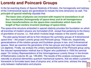
94. Rotations in the three spatial dimensions are examples of Lorentz transformations in
this generalized sense. They are of the form:
where Ri
j denotes ordinary 3×3 rotation matrices.
94
Lorentz boost with velocity v along the x
coordinate axis.
2017
MRT
Of more interest are special Lorentz transformations which mix
spatial coordinates with the time coordinate. The simplest of
these is a Lorentz boost along a given coordinate axis, say the
x-axis:
This corresponds physically to the transformation between two
coordinate frames moving with respect to each other along the
x-direction at the speed v=|v|=ctanhζ (with v being the velocity)
(see Figure). When relativistic motion (i.e., a proper Lorentz
boost) is along the y- or z- directions, the coshζ and sinhζ terms
move on to the appropriate row and column as shown above.












=
0
0
0
0001
][ i
jR
R µ
ν












=
1000
0100
00coshsinh
00sinhcosh
][ 1
ζζ
ζζ
µ
νL
t x y z
t
x
y
z
v
x,x
z
y y
z
O O

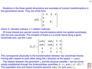
95. The relation between the rapidity parameter ζ and the physical speed variable v can
be conveniently established through the dimensionless quantities:
95
Interpretation of the Lorentz boost as a rotation
in the x0-x1 plane (with x0 = ict and x1=x).
2017
MRT
x
x
ict
ict
iζ
O
iζ
γζγβζ == coshsinh and
Substituting these results into our last matrix for [L1]µ
ν we get the usual*:
The hyperbolic sine and cosine functions become:
2
1
1
β
γβ
−
== and
c
v












=
1000
0100
00
00
][ 1
γγβ
γβγ
µ
νL
The parametrization in terms of hyperbolic functions is,
however, useful in emphasizing the similarity between rotations
and special Lorentz transformations. Thus a Lorentz boost along
the x-axis by a speed v can be interpreted as a rotation in the x0-
x1 plane by the hyperbolic angle (see Figure):






= −
c
v1
tanhζ
* Sometimes you have to be very careful with the signs of these matrices. Since I’m using
Wu-Ki Tung’s convention with x0 = ict (N.B., usually this is differentiated by naming this
coordinate x4 like Minkowski did) we have βγ . But when x0 = ct we would have −βγ .

96. From our matrix for [L1]µ
ν we can derive the Lorentz transformation formula for [x,t]
explicitly in terms of the velocity v between two coordinate frames moving relative to
each other along the x-axis.
Under a boost in the direction of the x-axis, [x,t]→[x,t]. Since the y and z components
are not affected, we will suppress them in what follows. Using our matrix [L1]µ
ν and the
fact that sinhζ =βγ and coshζ =γ, we have:












=





x
t
x
t
γγβ
γβγ
Carrying out the matrix multiplication, we get the following pair of equations:
xtt γβγ +=
Expressing β and γ in terms of the relative velocity v, we obtain:
22
11 







−
+
=








−
+
=
c
t
c
x
x
c
x
c
t
t
v
v
v
v
and
and
xtx βγβ +=

97. 97
vu •+−==⋅ ∑ 00
vuvugvu
µν
νµ
µν
2017
MRT
A general Lorentz transformation can be written as the product of rotations and
Lorentz boosts.
Proper Lorentz Group
The set of all proper Lorentz transformations {ΛΛΛΛ} satisfying Σµν gµν Λµ
λΛν
σ =gλσ given
Λ0
0≥1 forms the Proper Lorentz Group. It will be denoted by the symbol L+.
~
The group of all special ‘orthogonal’ 4×4 matrices – the quotation marks here call
attention to the non-Euclidean signature of the invariant metric gµν, (−1,1,1,1). Thus, Λ-
matrices for Lorentz boosts are not unitary like the rotation matrices. The mathematical
designation of this group is SO(3,1) where the arguments refer to the fact that the
signature of the metric tensor gµν involves 3 positive signs and 1 negative sign.
The scalar product of two four-vectors uµ and vµ is defined as:
The ordinary 4 components of a Lorentz vector {vµ} are referred to as the
contravariant components of v. An alternative way to represent the same vector is by its
covariant components {vµ} defined as:
∑=
ν
ν
µνµ vgv
It is obvious that v0 =−v0 and vi =vi for i=1,2,3. The scalar product above simplifies to:
∑∑ ==⋅
µ
µ
µ
µ
µ
µ vuvuvu

98. 98
2017
MRT
Making use of xµ =Σν Λµ
ν xν and vµ =Σν gµνvν, we have:
∑ −
Λ=→
ν
ν
ν
µµµ vvv ][ 1
∑∑∑∑ −
=Λ=Λ==
ν
ν
ν
µ
λσν
ν
σνλ
σµλ
λσ
σλ
σµλ
λ
λ
µλµ vvggvgvgv ][)( 1
ΛΛΛΛ
where the last step follows from ΛΛΛΛ−1=gΛΛΛΛTg−1. This means that the covariant components
of a four-vector v≡vµ transforms under proper Lorentz transformation as:
This result displays the transformation property of vµ in the form which most explicitly
indicates why Σµvµ uµ is an invariant. There is a natural covariant four-vector, the four-
gradient ∂µ . We can verify that:
∑∑ ∂
∂
Λ=
∂
∂
∂
∂
=
∂
∂
=∂→∂ −
λ
λ
λ
µ
λ
λµ
λ
µµµ
xxx
x
x
][ 1

99. 99
µµµµ
axxx +=→
2017
MRT
Lorentz transformations are homogeneous transformations on the four-dimensional
coordinates. The assumption of homogeneity of space-time requires the invariance of
the laws of physics under four-dimensional translations T(a) which are inhomogeneous
transformations:
Translations and the Poincaré Group
The four-dimensional translation group is Abelian.
Now, the set of transformations in Minkowski space consisting of all translations and
proper Lorentz transformations and their products for a group P, called the Poincaré
group, or the inhomogeneous Lorentz group. A general element of the Poincaré group is
denoted g(a,Λ), it induces the coordinate transformation:
µ
ν
νµ
ν
µµ
axxx a
+Λ= → ∑),(ΛΛΛΛg
A transformation g(ΛΛΛΛ,a) followed by another g(ΛΛΛΛ,a), is equivalent to a single
transformation given by the group multiplication rule:
),(),(),( aaaa += ΛΛΛΛΛΛΛΛΛΛΛΛΛΛΛΛΛΛΛΛ ggg
This can be seen by applying the transformation xµ →xµ above a second time for xµ →xµ:
)()( µ
λ
λµ
λ
λν
νλ
ν
µ
λ
µ
λ
λ
ν
νλ
ν
µ
λ
µ
λ
λµ
λ
µ
aaxaaxaxx +Λ+ΛΛ=+








+ΛΛ=+Λ= ∑∑∑ ∑∑
or x =ΛΛΛΛx+a=ΛΛΛΛ(ΛΛΛΛx+a)+a=(ΛΛΛΛΛΛΛΛ)x+(ΛΛΛΛa+a) if we suppress the Lorentz indices (and
the associated sum over repeated indices).
~
¯
¯

100. 100
















→
















Λ
→
110000
)(
),(
3
2
1
0
3
2
1
0
x
x
x
x
x
a
a
a
a
a µ
µ
ν
and
v
g ΛΛΛΛ
2017
MRT
As in the case of the E3 group, the (inhomogeneous) Poincaré group action (i.e., x→
x=Λx+a) can be cast in the form of an (homogeneous) matrix multiplication by the
following device:
A general element of the Poincaré group can be written in the factorized form:
)()(),( aa Tvg ΛΛΛΛΛΛΛΛ =
where T(a)=g(1, a) (where 1 is the trivial element or unit matrix) is a translation, and ΛΛΛΛ(v)
=g(ΛΛΛΛ,0) is a proper Lorentz transformation – a function of the velocity v of the particle.
Now, if we let ΛΛΛΛ be an arbitrary proper Lorentz transformation and T(a) a four-
dimensional translation, then the Lorentz transformed translation is another translation:
)()( 1
aa ΛΛΛΛΛΛΛΛΛΛΛΛ TT =−
and the group of translations forms an invariant subgroup of the Poincaré group.

101. 101
∑−=
µ
µ
µ
δδ Paia 1T )(
2017
MRT
The Poincaré group has ten generators – one for each of its independent one-parameter
subgroups. We consider first those associated with infinitesimal translations.
Generators and the Lie Algebra
The covariant generators for translation {Pµ} are defined by the following expression
for infinitesimal translations:
where 1 is the unit matrix and {δ aµ} are components of an arbitrary small four-
dimensional displacement vector. The corresponding contravariant generators {Pµ} are
defined by Pµ =Σν gµνPν so that P0 =−P0 and Pi =Pi. The generator for time translations P0
with be shown to relate to the energy operator – or Hamiltonian H – in physics. In that
context, we shall refer to P={Pµ} collectively as the four-momentum operator. As usual,
finite translations can be expressed in terms of the generators by exponentiation:
∑−
= µ µ
µ
Pai
aT e)(
Under the Lorentz group, the generators {Pµ} transform as four-coordinate unit vectors:
for all ΛΛΛΛ∈L+. Correspondingly, the covariant generators {Pµ} transform as:
∑Λ=−
ν
ν
ν
µµ PP 1
ΛΛΛΛΛΛΛΛ
~
∑ −−
Λ=
ν
νµ
ν
µ
PP ][ 11
ΛΛΛΛΛΛΛΛ

102. 102
∑−=
µν
µν
µν
δδ M
i
ω
2
)ω( 1ΛΛΛΛ
2017
MRT
The covariant generators for Lorentz transformations {Mµν} are anti-symmetric tensors
defined by the following expression for infinitesimal rotations in Minkowski space:
where δωµν =−δωµν are anti-symmetrical infinitesimal parameters. The corresponding
contravariant generators are:
∑=
λσ
σν
λσ
µλµν
gMgM
Hence, with m=1,2,3 we have M0m =−M0m =Mm0 and Mmn =Mmn.
∑∑ ==
k
k
knmnm
nm
nm
nmkk JMMJ εε and
A spatial rotation in the (m,n) plane can be interpreted as a rotation around the k-axis
when (k,m,n) is some permutation of (1,2,3). In previous chapters we have used the
notation R(δθ)=1−iΣkδθ kJk. Comparing with ΛΛΛΛ(δω)=1−(i/2)ΣµνδωµνMµν we can make
the identification δθ 1=δω23 and J1=M23 plus cyclic permutations. In a more compact
notation, we can write:
The association of rotation in the (m,n) plane with a unique axis (k) perpendicular to
that plane is a special property of three-dimensions. In the four-dimensional
Minkowski space, the subspace perpendicular to a plane is multi-dimensional – there
is no unique axis associated with a set of one-parameter rotations.
ˆ

103. 103
∑−=
m
m
m
Ki ζδζδ 1)(ΛΛΛΛ
2017
MRT
The three generators of special Lorentz transformations (or Lorentz boosts) mix the
time axis with one of he spatial dimensions. When focusing on this class of
transformations, we shall use the notation δζ m=δωm0 and Km=Mm0. Hence:
The 4×4 matrices for Km can be derived in the same way as for Jm, making use of
expressions of Lorentz boosts such as [L1]µ
ν , specialized to infinitesimal
transformations. As an example, we obtain:












=












=
0000
0000
0001
0010
0000
0000
000
000
][ 1 i
i
i
K µ
ν
and likewise for the other generators. Finite Lorentz boosts assume the familiar form:
∑−
=Λ m m
m
Ki ζ
ζ e)(
Similarly, the general proper Lorentz transformation can be written as:
∑−
=Λ νµ µν
µν
M
i
ω
2e)ω(
where ωµν is a six-parameter anti-symmetric second-rank tensor.
t x y z

104. 104
)ω()ω( 1
Λ=ΩΛΩ −
2017
MRT
The transformation law of Lorentz generators is given next if we let Λ(ω) be a proper
Lorentz transformation parameterized as in Λ(ω)=exp[−(i/2)Σµνωµν Mµν], and Ω be
another arbitrary Lorentz transformation, then:
where ωµν =Σλσ Ωµ
λ Ωµ
σ ωλσ . The generators {Mµν} transform under Ω as:
∑ ΩΩ=ΩΩ −
λσ
λσ
σ
ν
λ
µµν MJ 1
which states that, under proper Lorentz transformations, Mµν transforms as components
of a second rank tensor.
The Lie algebra of the Poincaré group is given by:
)(],[0],[ σµλλµσλσµνµ PgPgiJPPP −== ,
)(],[ νλµσνσµλµλσνλνµσλσµν MgMgMgMgiMM −+−=
and
To gain insight on these commutation relations, we separate the spatial and time compo-
nents and rewrite the Lie algebra in terms of the more familiar quantities {P0,Pm,Jm,Km}.
For the first [Pm,Pn]=0 we have [P0,Pm]=[Pn,Pm]=0. The second commutator is decom-
posed into [P0,Jn]=0, [Pm,Jn]=iΣl εmnlPl, [Pm,Kn]=iδ mn P0, and [P0,Kn]=iPn with these last
two stating that translations and Lorentz boosts in different direction spatial directions
commute but they mix if both involve the same direction in space. Finally, the third
commutator leads to [Jm,Jn]=iΣlεmnl Jl, [Km,Jn]=iΣlεmnlKl, and [Km,Kn]=−iΣlε mnl Jl.

105. 105
22
01 P−=−≡ ∑ PPPC
µ
µ
µ
2017
MRT
To study the unitary irreducible representation of the Poincaré group, we shall use
exclusively the method of induced representation, as it brings out features of the
representations which are manifestly related to physical allocations. In fact, the natural
correspondence between the basis vectors of unitary irreducible representations
of P and quantum mechanical states of elementary physical systems stands out
as one of the remarkable monuments to unity between mathematics and physics.
Representation of the Poincaré Group
~
The induced representation method is based on the use of the Abelian invariant
subgroup of translations {T4: T(a)}. The basis vectors will be chosen as eigenvectors of
the generators of translation Pµ, along with commutating operators chosen from the Lie
algebra of the relevant little group. The eigenvalues of Pµ will be denoted by pµ. Our
experience with the Euclidean groups suggest that the square of the four-momentum is
a Casimir operator which commutes with all generators, hence all group
transformations. We define this operator as:
Likewise, the eigenvalues of C1 will be denoted by c1. The irreducible representation
of P are labelled, among other indices, by c1. So, we shall consider basis vectors with a
definite linear momentum vector pµ which is related to c1 by:
~
∑−=
µ
µ
µ ppc1

106. Light-cone.
2017
MRT
Recall that with respect to an arbitrary chosen coordinate
origin, space-time is divided into three distinct regions separated
by the light-cone which is defined by the equation (see Figure):
0)(0 2022222
=−=− xctc xx or
106
0
0
0
0
1
1
1
0
1
<
≠=
>
===
cp
cp
cp
pcp
:vectorlike-Space
and:vectorlike-Light
:vectorlike-Time
and:vectorNull
0p
0p
We must distinguish between the following four cases:
The future cone consists of all points with |x|2 <0 and cx 0 >0.
These points can be reached from the origin by the world-line of
an evolving event. For the past cone, it consists of all points with
|x|2 <0 and cx0 <0. They represent events on world-lines which
can, in principle, evolve through the origin. By a suitable Lorentz
transformation, the coordinates of any point in these two regions
can be transformed into the form [ct,0]; hence these coordinate
vectors are said to be time-like.
x
cx0
Time-like
Future
cone
Past
cone
Time-like
Space-like Space-like
Light-like
Light-like
The region outside the light-cone is characterized by |x|2 >0.
For any given point in this region, there exists some Lorentz
transformation which transforms the components of the
coordinate vector into the form [0,x]. Hence there coordinate
vectors are said to be space-like and the entire region is called
the space-like region.

107. 107
∑ 0=00=0 0
j
j
j
mj
j
mj
mj
j
jjj mjmjmjmja ,;)]([,;,;,;)(
)(
v1T
v
ΛΛΛΛΛΛΛΛ Dand
2017
MRT
The null vector κµ =0 is invariant under all homogeneous Lorentz transformations. In
the terminology of the induced-representation method, the little group of p is the full
Lorentz group L+. Each irreducible unitary representation of the group L+ (characterized
by j0 and |v|) induces an irreducible unitary representation of the Poincaré group. Basis
vectors of such a representation are eigenvectors of [Pµ;J 2,J3] with eigenvalues [κ µ =0;
j, mj]. They satisfy the defining equations:
~ ~
where D( j0v)[Λ] are the unitary representation matrices of the homogeneous Lorentz
group. Physically, this null vector represents the vacuum in some way or another.
For a given positive c1 =−Σµ pµ pµ =(moc)2,we pick a time-likestandard vector kµ =[p0,p]
=[moc,0]. Physically, this corresponds to a state at rest (p=0) with mass or rest energy
equal to mo. The little group of L+ is SO(3). The basis vectors of the subspace
corresponding to the eigenvalues kµ of Pµ will be denoted by {|0mj 〉} where 0 refers to p
=0. Two implicit indices p0 =moc and J 2 =j( j+1) were suppressed (otherwise states would
be denoted as {|moc, j;pmj 〉}). The defining equations for these vectors are:
~
jjjjjjj mmmJmjjmmkmP 0000J00 =+== 3
2
)1(, andµµ
where kµ =[moc,0]. Recall that j corresponds to the intrinsic spin and mj is the
eigenvalue of the operator J•P/|p| hence it corresponds to the angular momentum
along the direction of the motion, or, in special cases, the helicity σ of the state
when the rest mass of the particle is zero (i.e., mo=0).

108. 108
1
3 ),,()()0,,( −
= ψθϕζβα RLRΛΛΛΛ
2017
MRT
To generate a complete set of basis consisting of general eigenvectors of Pµ, we
operate on |0mj 〉 by the remaining transformations of the factor group. A general element
of the proper Lorentz group L+ can be uniquely written in the factorized form:
where L3(ζ ) is a Lorentz boost along the positive z-axis by the velocity v=ctanhζ, 0≤ζ<∞,
and the Euler angles for the rotations have their usual ranges. Realizing that the first
rotation factor on the right-hand side of the above equation leaves the subspace
associated with the standard vector invariant, one need only consider the Lorentz boost
L3(ζ ) followed by a rotation R(α,β,0). We define:
~
jj mLmp 0z )(ˆ 3 ζ=
where p=mosinhζ is the magnitude of the three-momentum of the state. Then:
jjj mpLmpRm 0zp )(ˆ)0,,( == βα
where [β,α] are the polar and azimuthal angles of the momentum vector p. The Lorentz
transformation L(p) introduced above is:
)()0,,()( 3 ζβα LRpL =
will be referred to frequently in what follows. It transforms the rest frame vector kµ to a
general pµ.

109. 109
∑
∑
′
−′
′
′−
′ΛΛ∝=
′ΛΛ==
∑
∑
j
j
j
j
j
j
m j
paim
m
j
jj
m j
m
m
j
jj
pai
j
mpmaTmaU
mpmmma
pWpvp
pWpppT
µ µ
µ
µ µ
µ
e)],([)()(),(
)],([e)(
)(
)(
D
D
ΛΛΛΛΛΛΛΛ
ΛΛΛΛ
or
and
2017
MRT
The basis vector {|pmj 〉} describe above span a vector space which is invariant under
Poincaré group transformations. The action of group transformations on these basis
vectors is given by:
where the Wigner rotation is given by W(Λ,p)=L−1(Λp)ΛΛΛΛL(p) and the representation
matrix of the SO(3) group by D( j)[R] which also allows the correspondence to the angu-
lar momentum j (N.B., the states |Λpmj 〉 can be represented by |pmj 〉 using pµ=Σν Λµ
ν pν ).
We arrived at these results above in the following way:
∑
∑∑
∑
′
′
−−
−
′ΛΛ=
ΛΛ=ΛΛ==
===
===
j
j
j
m
j
m
m
j
jjjj
jjj
jjjj
mp
mpLpLmpLpLpLmpLm
mpmkpLmpLkpL
mPpLpLmpLPpLpLmpLPmP
pW
p00p
pp0
000p
)],([
)]()([)()()()(
)]([)()]([
)]([)()]()()[()(
)(
11
1
D
ΛΛΛΛΛΛΛΛΛΛΛΛΛΛΛΛ
andµ
ν
νµ
ν
ν
νµ
ν
ν
νµ
ν
µµµ
where Λp and W(Λ,p) are the same as defined above.

110. 110
∑≡
µνσ
σµν
λµνσλ
ε PMW
2
1
2017
MRT
The irreducible representations we just derived carry the label [moc, j]. The ‘rest mass’
parameter mo is the square root of the eigenvalue of the Casimir operator C1 =−ΣµPµ Pµ. It
is natural to ask: How is the ‘spin’ parameter j related to a second, as yet
unspecified, Casimir operator?
In the subspace corresponding to p=0, the parameter j is directly related to the eigen-
value of the operator J 2. J 2 commutes only with the generators of the little group of p=0
– it is certainly not invariant in general. The Casimir operator we are looking for must
fulfil the following requirements: 1) it is translationally invariant; 2) it is a Lorentz scalar;
and 3) it reduces to J 2 when c1
2 =(moc)2 >0. Condition 3 indicates that this operator is a
compound object quadratic in Mµν . Condition 2 might the suggest a Lorentz scalar in the
form of the product Mµν Mµν . This is, however, now a viable choice because it does not
satisfy condition 1 nor 3. We must look for an expression somewhat less obvious and to
this effect there is only one independent non-trivial choice – the Pauli-Lubanski vector:
which has the following properties:
)(],[0],[0 νλµµλνµνλµλ
λ
λ
λ
WgWgiJWPWPW −===∑ ,,
∑=
µν
νµ
λµνσσλ
ε PWiWW ],[
and

111. 111
∑≡
λ
λ
λ
WWC2
2017
MRT
The operator:
commutes with all generators of the Poincaré group. It is, therefore, a Casimir operator.
To gain some physical insight about {Wλ}, consider the vector space corresponding to
the [moc, j] representation discussed earlier. When operating on the basis vectors –
which are eigenstates of {Pµ} – we can replace {Pµ} with their eigenvalues. Thus, we
have Wλ =½Σµνσ ε λµνσ Mµν Pσ . In the subspace corresponding to the standard vector of
the physical system with p0 =moc and p=0, we have:
i
jk
kj
kjii
JcmM
cm
WW o
o0
2
0 === ∑εand
In other words, the independent components of the four-vector W are proportional to the
generators {Ji} of the little group.

112. 112
],0,0,[ κκµ
=k
2017
MRT
When Σµ pµ pµ =0, the magnitude of the time component pµ and the spatial three-vector
|p| are equal. This is typified by the four-momenta of photons, or equivalently the four-
wavevector of light propagators. Hence this case is termed light-like. Light-like four-
vectors do not have a rest-frame. The velocity of physical states with light-like momenta
remains constant at the value v=|p|/p0=1 (in units of c, the velocity of light) in all Lorentz
frames.
Since a standard light-like vector must have equal time and spatial components, it is
customary to pick it as:
where κ is an arbitrary fixed scale. To obtain a general state of momentum pµ =[ω,p]
where p=ωp and the unit vector p is characterized by the angles [θ,ϕ], we first apply a
Lorentz boost L3(ζ ) to transform the energy from κ to ω, then apply a rotation R(ϕ,θ,0)
to bring the z-axis into the p-direction. As before, we shall denote the transformation from
kµ to pµ by L(p):
ˆ ˆ
ˆ
∑∑ ==
ν
νµ
ν
ν
νµ
ν
µ
ζθϕ kLRkpLp )]()0,,([)]([ 3

113. 113
)()( 103122023112
30
MMWMMWMWW −=+=== κκκ and,
2017
MRT
The generators of the little group of the standard vector kµ are independent
components of the corresponding Pauli-Lubanski vector for kµ:
∑=
µνσ
σµν
λµνσλ
ε kMW
2
1
We obtain:
or, since M12 =J3, M23 =J1, M31 =J2, M20 =K2, and M10 =K1:
)()( 1222113
30
KJWKJWJWW −=+=== κκκ and,
The second Casimir operator is given by:
2
2
2
12 )()( WWWWC +== ∑λ
λ
λ
The Lie algebra is:
03
2
3
23300
3
3
0
0
=+−=+−=+=∑ JJkWkWkWkWkW κκ
λ
λ
λ
0],[ 21
=WW
as expected and similarly:
as well as:
2
3
11
3
2
],[],[ WiJWWiJW −== and

114. 114
01113111 === σσσσσσ µµ
ppppp iWJpP and,
2017
MRT
With W1,2 replaced by P1,2 we recognize this algebra as being the same as that of the
Euclidean group in two-dimensions, E2. In the Euclidean Groups E2 and E3 chapter the
irreducible unitary representations of the E2 group has degenerate representations that
correspond to w=0 which are one-dimensional with basis |mj 〉 labelled by mj , the
eigenvalue of J3. The non-degenerate representations correspond to w>0, they are all
infinite-dimensional and the basis vectors can be chosen as {|w mj 〉,mj =0,±1,…}.
Starting from any of these representations, we can generate a basis for a corresponding
representation of the full Poincaré group, labelled by mo (which is equal to zero) and w,
by applying the homogeneous Lorentz transformations L(p) (c.f., pµ =Σν[L(p)]µ
ν kν above)
to the basis vectors of the subspace.
In the physical world, no state corresponding to the [mo =0,w>0] representation are
known. On the other hand, the [mo =0,w=0,σ ] representations, with σ being the helicity,
are realized as photons (σ =±1), neutrino (σ =−1/2), and anti-neutrino (σ =1/2) states.
Hence, in the subsequent study, we shall confine ourselves to the degenerate case.
According to the above discussion, the subspace corresponding to the standard vector
p1 is one-dimensional and the basis vector |p1 σ〉 has the following defining properties:
where p1
µ=[κ,0,0,κ] and i=1,2. When σ is an integer, we obtain a single-valued
representation; when σ is an odd-half-integer, we obtain a double-valued representation.

115. 115
σζσσσθϕσ kzkzp )(ˆ)(ˆ)0,,( 3LppLpR === and
2017
MRT
The general basis vector is defined as:
where p=κ exp(ζ ) is the magnitude of p.
The basis vectors {|p σ〉} described above span a vector space which is invariant
under Poincaré group transformations. The resulting representation, labelled by [mo=0,
σ], is unitary and irreducible. The effect of the group transformations on these basis
vectors is:
σσσσ θσµ µ
µ
pppp Λ=Λ= Λ−− ∑ ),(
ee)( pipai
aT and
where θ(Λ,p) is an angle depending on Λ and p determined from the equation:
σσθσ
1
1
1
),(
)()(e pp pLpLpi
ΛΛ= −Λ−
As pointed out previously, |p σ〉 represents a state with momentum p and helicity σ .
Although there is a lot of similarity between these states with those of the time-like case,
one essential difference must be kept in mind: The helicity index σ is invariant under
Lorentz transformations for massless (light-like) states, whereas it is transformed among
all 2j+1 possible values for massive (time-like) states. In the literature, massless
particles corresponding to the [mo =0,±σ] representations are often said to have ‘spin-σ’
(e.g., photon with ‘spin-1’, neutrino with ‘spin-1/2’, &c.), a statement that can be very
misleading. It is referable to use the term helicity rather than spin when discussing
massless states where σ is invariant under all continuous space-time transformations.

116. 116
σσδδσσ )()( 3
pppp −= pN
2017
MRT
In applying the induced representation method we require all generators to be
represented by Hermitian operators. The basis vectors, defined as eigenvectors of a
maximal set of commuting generators, are orthogonal to each other by construction. We
shall now consider the proper normalization of these vectors.
Normalization of Basis States
where N(p) is a normalization factor yet to be determined. Substituting this last relation
into the above equation, we obtain the condition:
Because basis vectors corresponding to distinct eigenvalues must be mutually
orthogonal, we should have:
If the definition of the scalar product 〈p σ|p σ〉 is to be Lorentz invariant, we must
have:
∑ ΛΛΛΛ==
ττ
τ
σ
σ
τ ττσσσσ )],([)],([ )(†)(†
pp jj
WppWpppp DDΛΛΛΛΛΛΛΛ
)()()()( 33
pppp Λ−ΛΛ=− δδ pNpN
Any definition of N(p) which satisfies this requirement is said to provide a covariant
normalization for the states.

117. 117
∑ −
Λ=→
β
βα
β
α
ψψψψ )(][)(: 1
xx ΛΛΛΛΛΛΛΛ
D
2017
MRT
We emphasized earlier how physical states of definite mass and spin, labelled by their
momenta pµ and helicity σ, arise naturally from the irreducible representations of the
symmetry group of space-time – the Poincaré group. Traditionally, such states were not
derived this way but rather arose as elementary solutions to relativistic wave equations.
The most well-known among these are Maxwell’s equations (for spin-1 photons of elec-
tromagnetism), the Klein-Gordon equation (for spin-0 bosons), and the Dirac equation
(for spin-½ fermions). The components of the relativistic wave functions transform under
Lorentz transformations as finite-dimensional representations of the Lorentz group.
Wave Functions and Field Operators
Let { D[ΛΛΛΛ],ΛΛΛΛ≡Λµ
ν } be a finite-dimensional n×n matrix representation of the proper
Lorentz group. A c-number relativistic wave function is a set of n functions of space-time
{ψ α (x), x ≡ xµ} which transform under an arbitrary proper Lorentz transformation ΛΛΛΛ as:
For a given matrix representation { D[ΛΛΛΛ]} as above, a relativistic field operator is a set
of n operator-valued functions of space-time {ΨΨΨΨα(x)} which transforms under an arbitrary
proper Lorentz transformation ΛΛΛΛ as:
∑ Λ= −−
β
βα
β
α
)(][)()()( 11
xUxU ΨΨΨΨΛΛΛΛΛΛΛΛΨΨΨΨΛΛΛΛ D
where U(ΛΛΛΛ) is an operator representing ΛΛΛΛ on the Hilbert space where ΨΨΨΨ is defined. If
we also add translations then we have U(ΛΛΛΛ,a)ΨΨΨΨα(x)U−1(ΛΛΛΛ,a)=Σβ D[ΛΛΛΛ−1]α
β ΨΨΨΨβ(Λx+a).

118. 118
0)()],([ o =∂−Π∑β
βα
β xicm ΨΨΨΨh
2017
MRT
How is a field operator ΨΨΨΨα (x), transforming as U(ΛΛΛΛ)ΨΨΨΨα (x)U(ΛΛΛΛ−1)= Σβ D[ΛΛΛΛ−1]α
β ΨΨΨΨβ (Λ x),
made to describe a ‘particle’ of definite rest mass mo and spin j? The answer lies in
the wave equation ΨΨΨΨ(x) satisfies.
Relativistic Wave Equations
where Π is a linear differential operator(usually of the first or second degree in ∂µ =∂/∂xµ)
and it is a matrix with respect to the Lorentz index β of the wave equation.
0)(o =








+∂− ∑ xcmi ψγ
µ
µ
µ
h
where the four-component indices on the γ matrices and on ψ (x) have been
suppressed. The differential operator is linear in ∂ in this case. The simplest relativistic
wave equation is, however, the Klein-Gordon equation for spin-0 particles. The field
operator φ(x) has only one component and the differential operator Π is quadratic in ∂:
0)(
2
o
=














+∂∂− ∑ x
cm
φ
µ
µ
µ
h
Let us write the wave equation in the generic form:
An archetypical example of this operator equation is the Dirac equation for spin-½
particles:

119. 119
∫
∞
∞−
= h
h
xpi
p
pd
x e)(
)π2(
)( 3
4
ββ
ΦΦΦΦΨΨΨΨ
2017
MRT
The differential equation Σβ {Π[moc,−ih∂]}α
β ΨΨΨΨβ (x)=0 can be converted into an
algebraic equation by taking the Fourier transform:
We obtain:
0)(),()()],([ oo =Π≡Π∑ ppcmppcm β
β
βα
β ΦΦΦΦΦΦΦΦ
where the matrix indices are again suppressed. In order that Σβ {Π[moc,−ih∂]}α
β ΨΨΨΨβ (x)=
0 be a satisfactory relativistic wave equation for rest mass mo and spin j, the matrix
Π(moc,p) must have the following properties:
1. It is relativistically covariant, or:
),()(),()( o
1
o pcmpcm ΛΠ=Π −
ΛΛΛΛΛΛΛΛ DD
so that Π(moc,p)ΦΦΦΦβ (p)=0 above is unchanged under Lorentz transformations (i.e., the
validity of Π(moc,p)ΦΦΦΦ(p)=0 should guarantee that Π(moc,Λp)ΦΦΦΦ(Λp)=0);
2. The mass-shell condition:
0)(])([ 2
o
2
=+ pcmp ΦΦΦΦ
hence:
)(
~
])([)( 2
o
2
pcmpp ΦΦΦΦΦΦΦΦ += δ
must follow from Π(moc,p)ΦΦΦΦβ (p)=0; and
3. Π(moc,p) must act like a projection matrix to select out the desired spin components.

120. 120
2
o
20
)( cmp +±= p
2017
MRT
The last equation [p2 +(moc)2]ΦΦΦΦ(p)=0 implies that ΦΦΦΦ(p) is non-vanishing only when its
argument satisfies the mass-shell condition p2 +(moc)2 =0. There are two solutions to the
equation:
referred to as positive and negative solutions, respectively. Separating the two types of
solutions and making use of an invariant integration measure on the mass shell (e.g., dp
=[1/(2πh)3](d3p/2p0) – c.f., Tung, P. 202 or for another measure c.f., Weinberg, P. 67), we
can rewrite ΨΨΨΨβ (x)=∫±∞[d4p/(2πh)3]ΦΦΦΦβ (p) exp(ipx/h) as:
~
∫
∞
∞−
−
−
+ += ]e)(e)([
~
)( hh xpixpi
pppdx ΦΦΦΦΦΦΦΦΨΨΨΨ
where:
],)]c([[
~
)( 21
o
20
pp ±+±==± mpp ΦΦΦΦΦΦΦΦ
and ΦΦΦΦ is defined by ΦΦΦΦ(p)=δ [p2 +(moc)2]ΦΦΦΦ(p) obtained earlier. The matrix equations
satisfied by ΦΦΦΦ±(p) are:
~ ~
0)(),( o =±Π ± ppcm ΦΦΦΦ
where it is understood that any occurrence of p0 in Π is to be replaced by [p2 +(moc)2]1/2.
Hence Π(moc,p) is in reality only a function of the three-vector p. The occurrence of
negative energy solutions in relativistic wave equations is closely related to the
existence of an anti-particle state for each ordinary particle state and the associated
charge conjugation symmetry.

121. 121
0)(),( o =Π jmukcm 0β
2017
MRT
As an example, let us consider the case of the rest frame of a system where the
standard momentum is given by k=[moc,p=0]. In order that the wave equation describes
spin s article states, the matrix equation Π(moc,±p)ΦΦΦΦ±(p)=0 should have 2j+1
independent solutions corresponding to the mj =−j,−j+1,…,j states of the system in its
rest frame. We shall denote these elementary solution by u(0 mj ):
where mj =−j,…, j, andα and β (supressed on Π) are Lorentz indices. Once {u(0 mj )} are
specified, the general elementary solutions to Π(moc,±p)ΦΦΦΦ±(p)=0 can be written down:
∑=
β
βα
β
α
)()]([)( jj mupLmu 0p D
where L(p) is a Lorentz transformation which brings the rest-frame momentum vector k=
[moc,0] to the given p=[p0,p], such as that given by L(p)=R(α,β,0)L3(ζ ) (N.B., α and β
in R(α,β,0) are angles). To see that the wave function uβ(p mj ) above does satisfy the
wave function Π(moc,p)ΦΦΦΦβ(p)=0 obtained earlier, we note that:
)(),()]([
)()]([),()]([)(),(
o
1
oo
j
jj
mukcmpL
mupLkcmpLmupcm
0
pp
Π=
Π=Π −
D
DD
where the first step follows from D(Λ)Π(moc,p) D(Λ−1)=Π(moc,Λp), the second step from
uα (p mj)=Σβ D[L(p)]α
β uβ (0 mj ), and the third step from Σβ [Π(moc,k)]α
β uβ (0 mj )=0.
The elementary solutions given by uα (p mj )=Σβ D[L(p)]α
β uβ (0 mj ) above are
usually called plane wave solutions to the wave equation.

122. 122
2017
MRT
The general solution to the wave equation is a linear combination of the elementary
solutions. Taking this into account,we rewrite:
]e)()(e)()([
~
)(
44444 344444 21
444 8444 76
4444 34444 21
444 8444 76
hh
termenergyNegativetermenergyPositive
xpi
jj
m
xpi
jj mvmamumbpdx
j
−
∞
∞−
+−
−−+= ∑∫
ΦΦΦΦΦΦΦΦ
ΨΨΨΨ pppp βββ
where b(p mj ) and a(−p mj ) is the expansion coefficient. This equation is usually referred
to as the plane wave expansion of the field operator ΨΨΨΨ(x). Since we have consider ΨΨΨΨβ (x)
as operators (on the Hilbert space of physical states), we must ask: Which factor on the
right-hand side of the above expansion carries the operator value? Since dp, uβ(p mj )
and vβ(−p mj ), and exp(±ipx/h) are all complex numbers, the coefficient functions b(p mj )
and a(−p mj ) must be operator-valued.
~
∫∫
∞
∞−
−•∞
∞−
•
=== ppppr
rp
rp
ddt
h
tx
tE
i
hi
)(
23
π2
23
e)(
)π2(
1
e),(
1
),()( h
h
ϕβ
ΦΦΦΦΨΨΨΨΨΨΨΨ
In PART III – QUANTUM MECHANICS we saw that the whole wave function is given
by the Fourier transforms from coordinate space r (represented by the wave function
ΨΨΨΨ(r,t)) to momentum space p (represented by the wave function ΦΦΦΦ(p,t) and vice versa):
where h=h/2π is Dirac’s constant and h is Planck’s constant.
General Solution of a Wave Equation
as:
∫
∞
∞−
+− += ]e)(e)([
~
)( hh xpixpi
pppdx ΦΦΦΦΦΦΦΦΨΨΨΨ

123. 123
2017
MRT
Note that we will be considering the usual theoretical physics convention of setting the
American measured constants (e.g., a Canadian knows what a cm is but needs to look
up what an erg is since Canadians – and most of the world – use the metric system
MKS, an acronym for Meters-Kilogram-Second):
Present notation Meaning Customary notation Value (CGS)
mo Mass of the electron mo
Energy moc2 510.99 KeV
Momentum moc 1704 gauss cm
Frequency moc2/h
Wave number moc/h
1/mo Length (Compton wavelength)/2π h/moc 3.8615×10−11 cm
Time h/moc2
e2 Fine-structure constant e2/hc 1/137.038
e2/mo Classical radius of the electron e2/moc2 2.8176×10−11 cm
1/moe2 Bohr radius ao =h2/moe2 0.52945 Å
to unity in what follows. But from what preceded you can substitute these back if you
ever have practical calculations to do or do as most physicists do which is to
correspond:
Present notation Meaning Customary notation Value (CGS)
c= 1 Speed of light in vacuum c 2.99793×1010 cm/s
h =1 Planck’s constant (h)/2π h 1.0544×10−11 erg/s
It’s obvious that it’s reasonable to assume that if you’ve made it this far you can look
up these American CGS values for yourself or convert them to MKS or XXI century
units if you wish.

124. 124
2017
MRT
The Poincaré states, |pmj 〉=R(α,β,0)|pzmj 〉=L(p)|0mj 〉, can be written in terms of
creation operators {a†(p mj )} as follows:
ˆ
0)(†
jj mam pp =
where |0〉 is the vacuum state. The transformation properties of the states |pmj 〉, ΛΛΛΛ|pmj 〉
=Σm′j
D( j)[W(ΛΛΛΛ,p)]mj
m′j
|Λpm′j 〉, imply for the operators:
∑′
′−
′ΛΛ=
j
j
j
m
j
m
m
j
j mapUmaU )()],([)()()( †)(1†
pWp DΛΛΛΛΛΛΛΛ
The Hermitian conjugates of the above equations are:
)(0 jj mam pp =
∑′
′
−−
′ΛΛ=
j
j
j
m
j
m
m
j
j mapUmaU )(]),([)()()( 1)(1
pWp DΛΛΛΛΛΛΛΛ
and:
and {a(p mj )} are the annihilation operators.
Creation and Annihilation Operators

125. 125
( )ϕϕψψ ββββ
)(0)()(0)( ppxx ΦΦΦΦΨΨΨΨ ==
2017
MRT
The coordinate space (i.e., a complex number) wave function of any physical state |ψ 〉
can be expressed as matrix elements of the field operator (c.f., 〈0|ΨΨΨΨ(x)|ψ 〉=ψ(x)):
where |0〉 is the vacuum state and ΨΨΨΨ(x)=ΨΨΨΨ(x,t) (and ΦΦΦΦ(p)=ΦΦΦΦ(p,t) for a momuntum space
wavefunction). Applying this connection to the linear momentum basis states, we obtain:
j
xpi
j mxm pp )(0e)(u ββ
ψ=
Substituting the plane wave expansionΨΨΨΨβ (x)=Σσ ∫±∞ dp[b(p mj)uβ(p mj)exp(ipx)+…] andthe
creation operators state |pmj 〉=a†(p mj )|0〉 in the right-hand side, we obtain the condition:
jjmmjj mmmama jj
pppppp ′=−=′ ′δδ )(
~
0)()(0 †
~
where δ(p−p) is the invariant delta function on the mass shell complementary to the
invariant measure of integration dp introduced earlier. It is now clear that the operator-
valued coefficient b(p mj ) are nothing other than the annihilation operators for the
corresponding basis states:
~
)()( jj mamb pp ≡
We go back to the plane wave expansion,ΨΨΨΨβ (x)=Σmj
∫±∞ dp[b(p mj )uβ (p mj )exp(ipx)+…],
and consider its significance. The field operator ΨΨΨΨβ (x) transforms as certain finite
dimensional non-unitary representation of the Lorentz group, whereas the annihilation
operator a(p mj ) transforms as the infinite dimensional unitary representation of the
Poincaré group characterized by [moc, j]. uβ (p mj )exp(ipx) is the glue between them.
~

126. 126
∑ ∑∫
∑ ∑∫
∑
′
∞
∞−
′
′
−
′
∞
∞−
Λ′
′
−
′
′
′
−−
−+ΛΛ=
−+=
Λ=
β
ββ
β
β
ββ
β
β
ββ
β
β
j
j
m
xpi
jj
m
xqi
jj
mumapd
mumaqd
xUxU
)](e)()([
~
][
)](e)()([
~
][
)(][)()()(
1
1
11
termenergy
termenergy
pp
qq
ΛΛΛΛ
ΛΛΛΛ
ΨΨΨΨΛΛΛΛΛΛΛΛΨΨΨΨΛΛΛΛ
D
D
D
2017
MRT
The complex number wave function uβ (p mj )exp(ipx) in the plane wave expansion
formula ΨΨΨΨβ (x)=Σmj
∫±∞ dp[b(p mj )uβ (p mj )exp(ipx)+…] are the coefficient functions which
connect the set of operators {a(p mj )}, transforming at the irreducible unitary
representation [moc, j] of the Poincaré group, to the set of field operators Ψβ(x),
transforming as certain finite dimensional non-unitary representation of the Lorentz
group.
~
To peruse this group theoretical interpretation of the plane wave solutions of the wave
equation a little further, note that uβ (p mj )exp(ipx) carries both the Poincaré indices (p mj )
and the Lorentz indices (x α). Applying a Lorentz transformation Λ to both sides of ΨΨΨΨβ (x)
=Σmj
∫±∞ dp[b(p mj )uβ (p mj )exp(ipx)+…] (this is termed the RHS), we obtain:
~
where in the last step, we made a change of integration variable from q to p=Λ−1q, and
we arrive at:
∑ ∫′
∞
∞−
′−−
−+′ΛΛ=
jj
j
j
mm
xpi
jj
m
m
j
mumappdUU
,
1)(1
)](e)()(]),([
~
)()( termenergyRHS ppW β
DΛΛΛΛΛΛΛΛ

127. 127
∑∑ ′
′−
′
′
′
−
′Λ=Λ
j
j
j
m
j
m
m
j
j mupmu )(]),([)(][ 1)(1
pWp β
β
ββ
β DD ΛΛΛΛ
2017
MRT
Comparing the two expressions, we obtain:
or, equivalently:
∑∑ ′
′
′
′
′ ′ΛΛ=
j
j
j
m
j
m
m
j
j mupmu )()],([)(][ )(
pWp β
β
ββ
β DD ΛΛΛΛ
This equation can be compared with one previously derived:
∑′
′
′ΛΛ=
j
j
j
m
j
m
m
j
j mpm pWp )],([)(
DΛΛΛΛ
where W(Λ,p)≡L−1(Λp)ΛΛΛΛL(p) and recognized as a realization of that formula since the
coefficient uβ(p mj ) is the plane wave solution corresponding to the state |p mj 〉 in the
chosen Lorentz group representation (with index α). The explicit expression for u(p mj )
given by uα(p mj ) =Σβ D[L(p)]α
β uβ(0 mj ) for an irreducible Lorentz wave function satisfies
Σβ ′ D[ΛΛΛΛ]β
β ′ uβ ′(p mj )=Σm′j
D( j)[W(Λ,p)]m′j
mj
uβ(Λp mj ) above.
The particle states are physical states, the associated representation (Poincaré) must
be unitary. On the other hand, the field operators ΨΨΨΨ(x) in physics are not always direct
physical observables, the corresponding representation (Lorentz) does not have to be
unitary. The reason for using the operators ΨΨΨΨ(x) in physics is that interactions between
fundamental particles are most conveniently formulated in terms of these field operators
if general requirements of covariance, causality, … &c. are to be incorporated in a
consistent way.

128. 2017
MRT
J.J. Sakurai, Modern Quantum Mechanics, Second Edition (Jim J. Napolitano), Addison-Wesley, 1994.
University of California at Los Angeles
This best-selling classic provides a graduate-level, non-historical, modern introduction of quantum mechanical concepts. The author,
J. J. Sakurai, was a renowned theorist in particle theory. This revision by Jim Napolitano retains the original material and adds topics
that extend the book’s usefulness into the 21st century. The introduction of new material, and modification of existing material,
appears in a way that better prepares readers for the next course in quantum field theory. Readers will still find such classic
developments as neutron interferometer experiments, Feynman path integrals, correlation measurements, and Bell’s inequality. The
style and treatment of topics is now more consistent across chapters. The Second Edition has been updated for currency and
consistency across all topics and has been checked for the right amount of mathematical rigor. Fundamental Concepts, Quantum
Dynamics, Theory of Angular Momentum, Symmetry in Quantum Mechanics, Approximation Methods, Scattering Theory, Identical
Particles, Relativistic Quantum Mechanics, Appendices, Brief Summary of Elementary Solutions to Shrödinger’s Wave Equation.
Intended for those interested in gaining a basic knowledge of quantum mechanics.
Wu-Ki Tung, Group Theory in Physics, World Scientific, 1985.
Michigan State University
An introductory textbook for graduates and advanced undergraduates on group representation theory. It emphasizes group theory’s
role as the mathematical framework for describing symmetry properties of classical and quantum mechanical systems.
“This book is written to meet precisely this need of the lack of suitable textbooks on general group-theoretical methods in physics for
all serious students of experimental and theoretical physics at the beginning graduate and advanced undergraduate level.” Physics
Briefs; “This book is well organized and the material is presented in an appealing and easily absorbed style, ... comes closer than any
other to being a modern version of Wigner’s classic Group Theory and its Application to the Quantum Mechanics of Atomic Spectra.”
Foundations of Physics; “A valuable addition to group theory texts for physicists. It is most appropriate for students who have taken
or are taking graduate quantum mechanics, especially if their interests lie in modern field theory.” Mathematical Reviews.
Steven Weinberg, The Quantum Theory of Fields, Volume I, Cambridge University Press, 1995.
Josey Regental Chair in Science at the University of Texas at Austin
Volume 1 (of 3) introduces the foundations of quantum field theory. The development is fresh and logical throughout, with each step
carefully motivated by what has gone before, and emphasizing the reasons why such a theory should describe nature. After a brief
historical outline, the book begins anew with the principles about which we are most certain, relativity and quantum mechanics, and
the properties of particles that follow from these principles. Quantum field theory emerges from this as a natural consequence. The
author presents the classic calculations of quantum electrodynamics in a thoroughly modern way, showing the use of path integrals
and dimensional regularization. His account of renormalization theory reflects the changes in our view of quantum field theory since
the advent of effective field theories. The book’s scope extends beyond quantum electrodynamics to elementary particle physics, and
nuclear physics. It contains much original material, and is peppered with examples and insights drawn from the author’s
experience as a leader of elementary particle research.
128
References / Study Guide

129. ...6180339887.1
2
51
01
1)1(
1
1
1
2
=
+
=
=−−
=−
−
=
ϕ
ϕϕ
ϕϕ
ϕ
ϕ
The Golden Ratio corresponds to the ratio of the sum of the quantities to the larger
one equals the ratio of the larger one to the smaller. The golden ratio is an irrational
mathematical constant, approximately 1.6180339887.
ϕ==
+
⇔
b
a
a
ba
The figure above illustrates the geometric relationship that defines this constant and is
expressed algebraically by an equation that has as a unique positive solution in an
algebraic irrational number. The Christian Bible describes the Ark of the Covenant as 1.5
cubits broad and high, and 2.5 cubits long conforming to the golden ratio!
Mathematically, this is the same thing as saying that ϕ is to 1 as 1 is to ϕ −1: