Downloaded 711 times
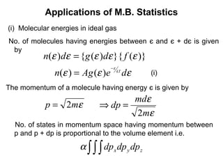
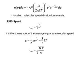
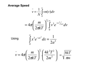
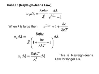
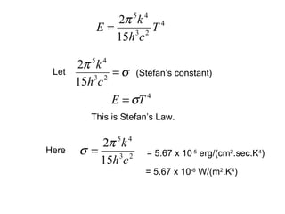
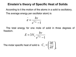
![Most Probable Speed
3
m 2 −mv2 2 kT
2
n(v) = 4πN ve
2πkT
[ ]
3
dn(v) m d 2 −mv2 2 kT
2
= 4πN ve =0
dv 2πkT dv
3
m
2
4πN ≠0
2πkT
dv
[
ve ]
d 2 −mv2 2 kT
=0 ⇒ vp =
2kT
m](https://image.slidesharecdn.com/statisticalmechanics-130416113806-phpapp02/85/Statistical-mechanics-15-320.jpg)
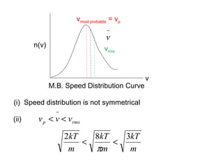
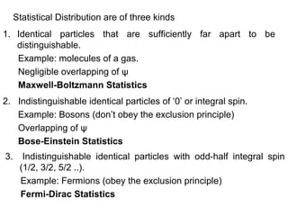
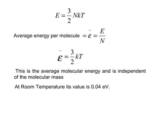
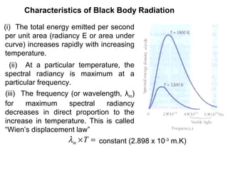
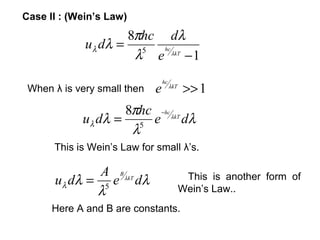
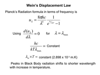
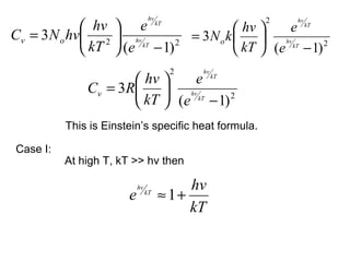
![Consider a system of two particles, 1 and 2, one of which is in
state ‘a’ and the other in state ‘b’.
When particles are distinguishable then
ψ ' = ψ a (1)ψ b (2)
ψ " = ψ a (2)ψ b (1)
When particles are indistinguishable then
1
For Bosons, ψ B = [ψ a (1)ψ b (2) +ψ a (2)ψ b (1)]
2
symmetric
1
For Fermions,ψ F = [ψ a (1)ψ b (2) −ψ a (2)ψ b (1)]
2
anti-symmetric](https://image.slidesharecdn.com/statisticalmechanics-130416113806-phpapp02/85/Statistical-mechanics-19-320.jpg)
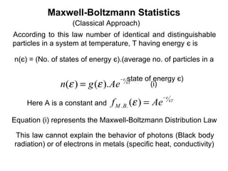
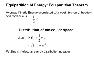
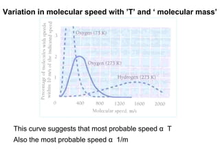
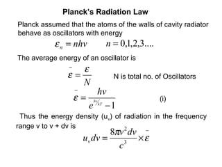
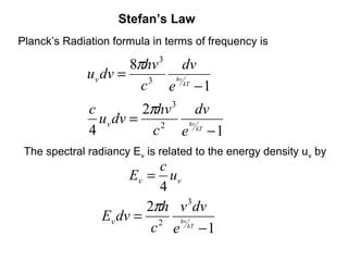
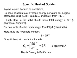
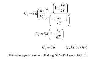
![ψF becomes zero when ‘a’ is replaced with ‘b’ i.e.
1
ψF = [ψ a (1)ψ a (2) −ψ a (2)ψ a (1)] = 0
2
Thus two Fermions can’t exist in same state (Obey Exclusion
Principle)](https://image.slidesharecdn.com/statisticalmechanics-130416113806-phpapp02/85/Statistical-mechanics-20-320.jpg)
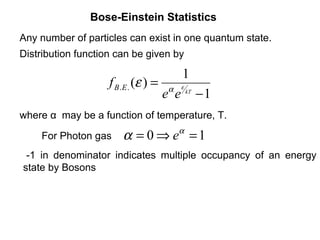
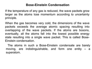
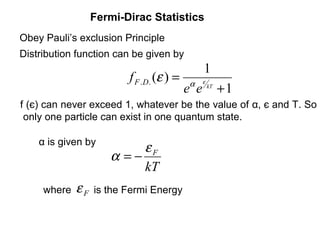
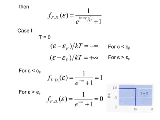
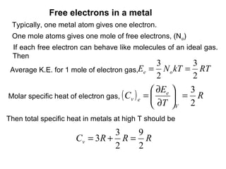
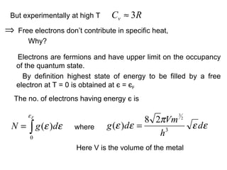
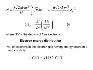


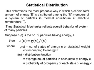
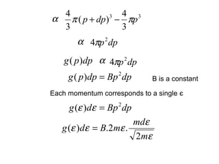
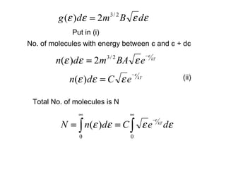
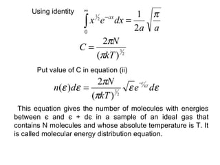
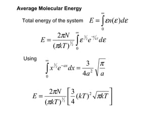
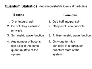
This document discusses statistical mechanics and the distribution of energy among particles in a system. It provides 3 main types of statistical distributions based on the properties of identical particles: Maxwell-Boltzmann, Bose-Einstein, and Fermi-Dirac statistics. Maxwell-Boltzmann statistics applies to distinguishable particles, while Bose-Einstein and Fermi-Dirac apply to indistinguishable particles (bosons and fermions respectively), with the key difference being that fermions obey the Pauli exclusion principle. The document also discusses applications of these distributions, including the Maxwell-Boltzmann distribution law for molecular energies in an ideal gas.