Download as PDF, PPTX

![Simulation of random variables
There is a lot of techniques and methods to
simulate r.v.
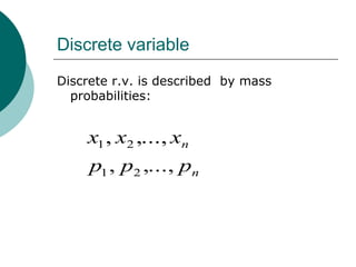
Let r.v. be uniformly distributed in the
interval (0,1]
Then, the random variable U , where
F (U ) ,
is distributed with the cumulative
distribution function F ( )](https://image.slidesharecdn.com/lecture2-100818112922-phpapp01/85/Basics-of-probability-in-statistical-simulation-and-stochastic-programming-20-320.jpg)

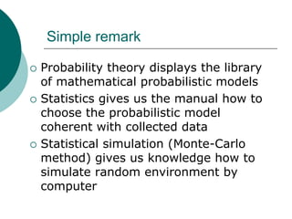
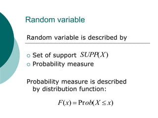
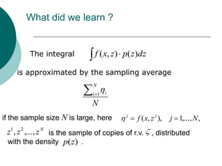
The document discusses the basics of probability in statistical simulation and stochastic programming, covering random variables, the law of large numbers, and the central limit theorem. It emphasizes the importance of probability theory and statistics in selecting appropriate probabilistic models and simulating random environments, particularly through methods like Monte Carlo simulation. Key points include approximating expectations of random functions and evaluating the reliability of statistical approximations using established theorems.