The document presents a detailed overview of the Jacobi iteration method used for solving systems of linear equations in numerical analysis. It covers the method's principles, numerical algorithm, implementation in C programming, advantages, and limitations. The Jacobi method is highlighted for its simplicity and robustness but noted for its inflexibility and potential convergence issues under certain conditions.

1. NORTH WESTERN UNIVERSITY
Computer Science & Engineering
Course Titel: Numerical Analysis
Course Code: CSE-2321
Presentation on: Jacobi Iteration Method
Submitted by:
Name : MD. MONIRUL ISLAM
ID: 20151116010
Submitted to:
Name : SONIYA YEASMIN
Lecturer
Computer Science & Engineering
North Western University , Khulna

2. * General Introduction of Jacobi Iteration Method.
* Basic idea of Jacobi Iteration Method.
* Numerical algorithm of Jacobi Iteration Method.
* Implementation of Jacobi Iteration Method in C Programming.
* Advantages of Jacobi Iteration Method.
* Limitations of Jacobi Iteration Method.
* References.
INDEX

3. General Introduction of Jacobi Iteration Method
Jacobi iterative method is considered as an iterative algorithm which is used for
determining the solutions for the system of linear equations in numerical linear algebra,
which is diagonally dominant.
In this method, an approximate value is filled in for each diagonal element. Until it
converges, the process is iterated. This algorithm was first called the Jacobi
transformation process of matrix diagonalization.
The Jacobi iteration is the simplest of the classical iterative methods and, generally, the
slowest. However, it forms a basis for the understanding of other methods, such as
Gauss-Seidel and SOR.

4. Basic idea of Jacobi Iteration Method
Two assumptions made on Jacobi Method:
1.The system given by
a11x1 +a12x2+… a1nxn=b 1
a21x1 +a22x2+… a2nxn=b 2
an1x1 +an2x2+… annxn =b n
Has a unique solution.
2.The coefficient matrix A has no zeros on its main diagonal, namely a11, a22,ann are nonzeros.
Main idea of Jacobi method :
To begin, solve the 1st equation for x1, the 2nd equation for x2 and so on to obtain the rewritten equations:

5. Then make an initial guess of the solution . Substitute these values into the right hand side the
of the rewritten equations to obtain the first approximation,
This accomplishes one iteration.
In the same way, the second approximation is computed by substituting the first approximation’s -
vales into the right hand side of the rewritten equations.
By repeated iterations, we form a sequence of approximations .
The Jacobi Method.
For each k ≤ 1, generate the components xi
(k) of x(k) from x(k-1) by,

6. Example: Apply the Jacobi method to solve,
Continue iterations until two successive approximations are identical when rounded to three significant digits.
Solution :To begin, rewrite the system
Choose the initial guess x1=0, x2=0 and x3=0 .
The first approximation is ,

7. Continue iteration, we obtain ,
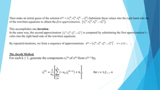
The Jacobi Method in Matrix Form
x1
Consider to solve an n×n size system of linear equations Ax=b with A= for x= [x2]
xn
We split A into,
Ax=b is transformed into (D-L-U)x = b .
Dx=(L+U)x + b.
Assume D-1 exist and D-1=

8. Then, x=D-1(L+U)x +D-1b.
The matrix form of Jacobi iterative method is ,
x(k) =D -1(L+U)x(k-1) +D -1 b k=1,2,3….
Define T=D-1(L+U) and c= D-1b Jacobi iteration method can also be written as ,
x(k) =Tx(k-1) +c k=1,2,3….

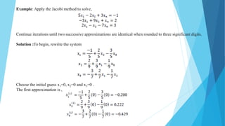
9. Numerical algorithm of Jacobi Iteration Method
Input: A=[aij] , b×XO= x0 , tolerance TOL, maximum number of iterations N.
Step 1: Set K=1
Step 2: While (k ≤ N) do step 3-6.
Step 3: For for i= 1,2,…n .
Step 4: If │ |x-X0| │< TOT Then OUTPUT (x1,x2,x3,..xn) ;
Step 5: Set k=k+1.
Step 6: For for i = 1,2,….n
Set XOi= xi
Step 7: OUTPUT (x1,x2,x3,…xn);
STOP
Another stopping criterion in Step 4:

10. Implementation of Jacobi Iteration Method in
C Programming
#include<stdio.h>
#include<conio.h>
#include<math.h>
float fx(float y,float z)
{
float x1; x1=4-2*y-3*z;
return x1;
}
float fy(float x,float z)
{
float y1;
y1=(8-5*x-7*z)/6;
return y1;
}
float fz(float x,float y)
{
float z1;
z1=(3-9*x-y)/2;
return z1;
}
void main()
{
int i,j,n;
float a1,b1,c1;
INPUT:

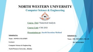
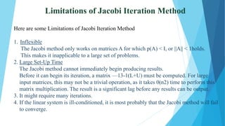
11. float a,b,c;
float ar[3][4],x[3];
clrscr();
printf("Enter the no. of Iteration : ");
scanf("%d",&n);
printf("Enter The initial value : ");
scanf("%f %f %f",&a,&b,&c);
for(i=0;i<n ; i++)
{
for(j=0;j<n ; j++)
{
a1=fx(b , c);
b1=fy(a , c);
c1=fz(a , b);
a=a1;
b=b1;
c=c1;
}
}
printf("a1 = %fn a2 = %fn a3 = %f",a1,b1,c1);
getch();
}
OUTPUT:

12. Advantages of Jacobi Iteration Method
Here are some advantages of Jacobi Iteration Method
1. It is simple and numerically robust.
2. Each iterations quite fast.
3. It is highly desirable for many applications.
4. The Jacobi method first generate inexact result and subsequently refines its result at
each iteration , with the residuals Converging at an exponential rate.

13. Limitations of Jacobi Iteration Method
Here are some Limitations of Jacobi Iteration Method
1. Inflexible
The Jacobi method only works on matrices A for which p(A) < I, or ||A|| < 1holds.
This makes it inapplicable to a large set of problems.
2. Large Set-Up Time
The Jacobi method cannot immediately begin producing results.
Before it can begin its iteration, a matrix —13-1(L+U) must be computed. For large
input matrices, this may not be a trivial operation, as it takes 0(n2) time to perform this
matrix multiplication. The result is a significant lag before any results can be output.
3. It might require many iterations.
4. If the linear system is ill-conditioned, it is most probably that the Jacobi method will fail
to converge.

14. References
[1] . Numerical Methods.by E Balaguruswamy.
[2] . https://www3.nd.edu/~zxu2/acms40390F12/Lec-7.3.pdf
[3] . https://en.wikipedia.org/wiki/Jacobi_method