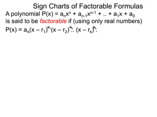
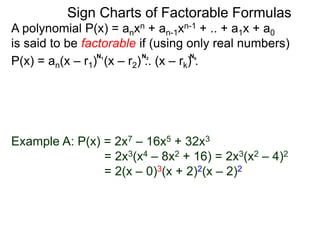
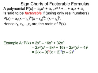
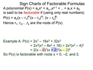
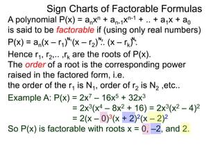
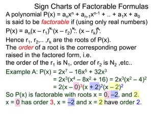
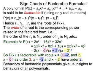
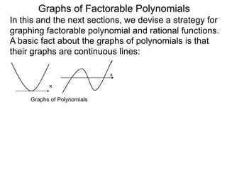
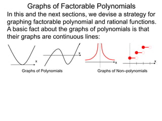
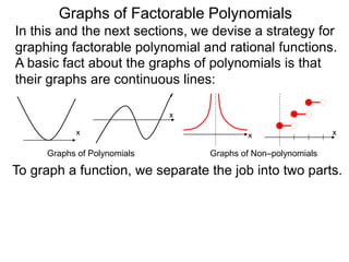
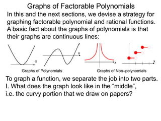
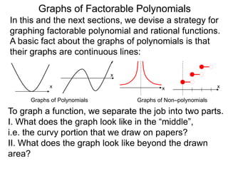
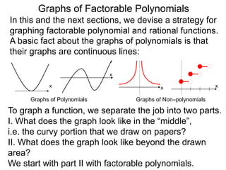
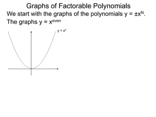
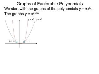
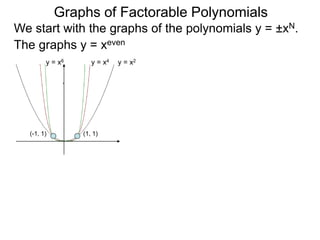
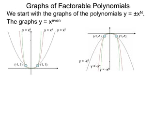
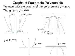
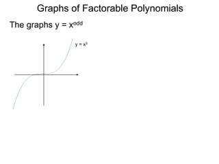
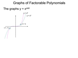
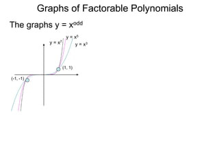
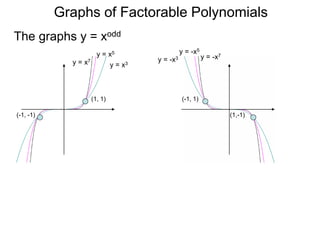
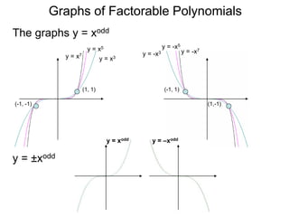
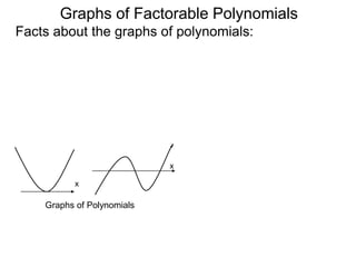
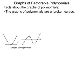
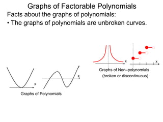
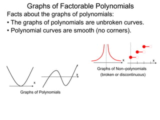
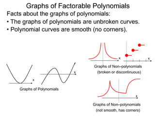
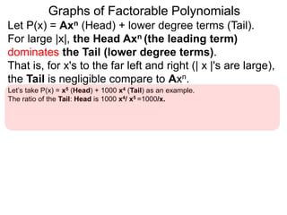
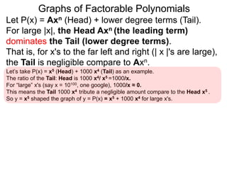
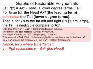
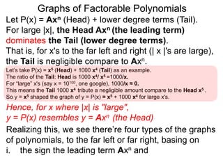
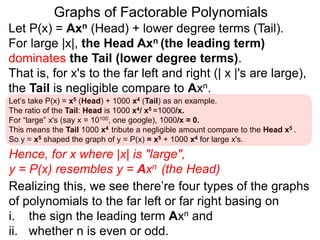
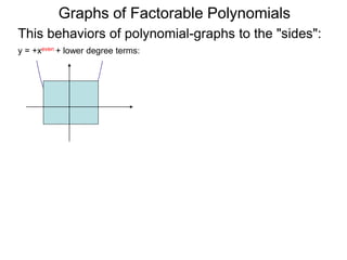
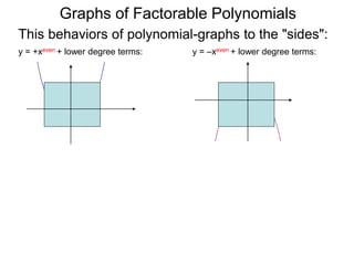
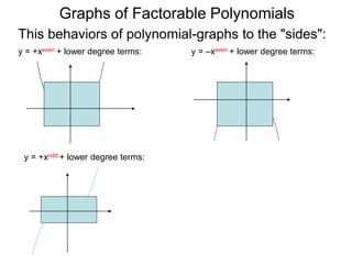
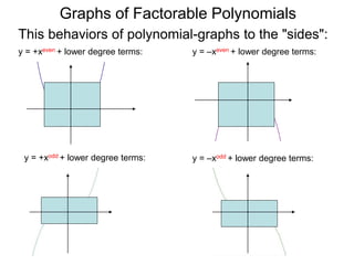
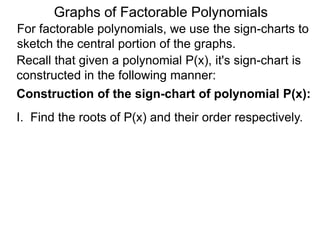
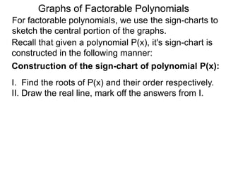
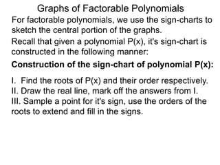
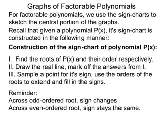
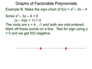
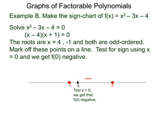
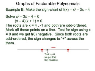
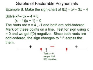
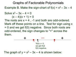
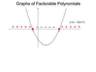
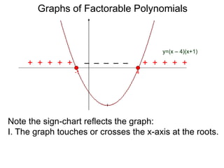
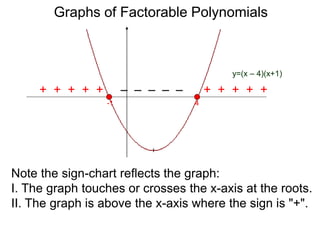
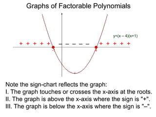
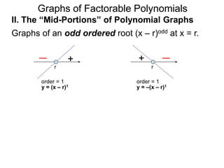
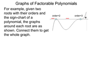
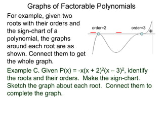
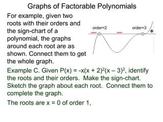
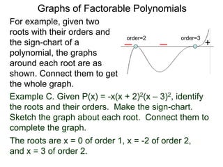
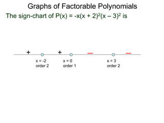
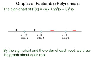
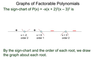
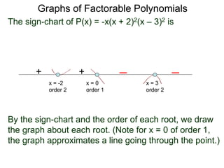
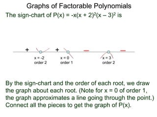
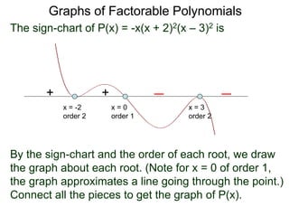
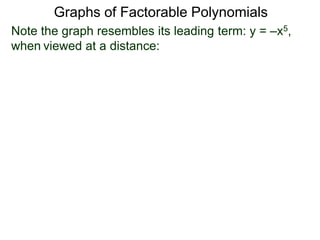
The document discusses factorable polynomials and how to graph them. It defines a factorable polynomial as one that can be written as the product of linear factors using real numbers. For large values of x, the leading term of a polynomial dominates so the graph resembles that of the leading term. To graph a factorable polynomial, one first graphs the individual factors like x^n and then combines them, which gives smooth curves tending to the graphs of the leading terms for large x.

1. Graphs of Factorable Polynomials
http://www.lahc.edu/math/precalculus/math_260a.html

2. Sign Charts of Factorable Formulas
A polynomial P(x) = anxn + an-1xn-1 + .. + a1x + a0
is said to be factorable if (using only real numbers)
P(x) = an(x – r1) (x – r2) .. (x – rk) .
N1 N2 Nk

3. A polynomial P(x) = anxn + an-1xn-1 + .. + a1x + a0
is said to be factorable if (using only real numbers)
P(x) = an(x – r1) (x – r2) .. (x – rk) .
N1 N2 Nk
Example A: P(x) = 2x7 – 16x5 + 32x3
= 2x3(x4 – 8x2 + 16) = 2x3(x2 – 4)2
= 2(x – 0)3(x + 2)2(x – 2)2
Sign Charts of Factorable Formulas

4. A polynomial P(x) = anxn + an-1xn-1 + .. + a1x + a0
is said to be factorable if (using only real numbers)
P(x) = an(x – r1) (x – r2) .. (x – rk) .
Hence r1, r2,.. ,rk are the roots of P(x).
N1 N2 Nk
Example A: P(x) = 2x7 – 16x5 + 32x3
= 2x3(x4 – 8x2 + 16) = 2x3(x2 – 4)2
= 2(x – 0)3(x + 2)2(x – 2)2
Sign Charts of Factorable Formulas

5. A polynomial P(x) = anxn + an-1xn-1 + .. + a1x + a0
is said to be factorable if (using only real numbers)
P(x) = an(x – r1) (x – r2) .. (x – rk) .
Hence r1, r2,.. ,rk are the roots of P(x).
N1 N2 Nk
Example A: P(x) = 2x7 – 16x5 + 32x3
= 2x3(x4 – 8x2 + 16) = 2x3(x2 – 4)2
= 2(x – 0)3(x + 2)2(x – 2)2
So P(x) is factorable with roots x = 0, –2, and 2.
Sign Charts of Factorable Formulas

6. A polynomial P(x) = anxn + an-1xn-1 + .. + a1x + a0
is said to be factorable if (using only real numbers)
P(x) = an(x – r1) (x – r2) .. (x – rk) .
Hence r1, r2,.. ,rk are the roots of P(x).
The order of a root is the corresponding power
raised in the factored form, i.e.
the order of the r1 is N1, order of r2 is N2 ,etc..
N1 N2 Nk
Example A: P(x) = 2x7 – 16x5 + 32x3
= 2x3(x4 – 8x2 + 16) = 2x3(x2 – 4)2
= 2(x – 0)3(x + 2)2(x – 2)2
So P(x) is factorable with roots x = 0, –2, and 2.
Sign Charts of Factorable Formulas

7. A polynomial P(x) = anxn + an-1xn-1 + .. + a1x + a0
is said to be factorable if (using only real numbers)
P(x) = an(x – r1) (x – r2) .. (x – rk) .
Hence r1, r2,.. ,rk are the roots of P(x).
The order of a root is the corresponding power
raised in the factored form, i.e.
the order of the r1 is N1, order of r2 is N2 ,etc..
N1 N2 Nk
Example A: P(x) = 2x7 – 16x5 + 32x3
= 2x3(x4 – 8x2 + 16) = 2x3(x2 – 4)2
= 2(x – 0)3(x + 2)2(x – 2)2
So P(x) is factorable with roots x = 0, –2, and 2.
x = 0 has order 3, x = –2 and x = 2 have order 2.
Sign Charts of Factorable Formulas

8. Behaviors of factorable polynomials give us insights to
behaviors of all polynomials.
A polynomial P(x) = anxn + an-1xn-1 + .. + a1x + a0
is said to be factorable if (using only real numbers)
P(x) = an(x – r1) (x – r2) .. (x – rk) .
Hence r1, r2,.. ,rk are the roots of P(x).
The order of a root is the corresponding power
raised in the factored form, i.e.
the order of the r1 is N1, order of r2 is N2 ,etc..
N1 N2 Nk
Example A: P(x) = 2x7 – 16x5 + 32x3
= 2x3(x4 – 8x2 + 16) = 2x3(x2 – 4)2
= 2(x – 0)3(x + 2)2(x – 2)2
So P(x) is factorable with roots x = 0, –2, and 2.
x = 0 has order 3, x = –2 and x = 2 have order 2.
Sign Charts of Factorable Formulas

9. Graphs of Factorable Polynomials
In this and the next sections, we devise a strategy for
graphing factorable polynomial and rational functions.

10. Graphs of Factorable Polynomials
In this and the next sections, we devise a strategy for
graphing factorable polynomial and rational functions.
A basic fact about the graphs of polynomials is that
their graphs are continuous lines:
x
x
Graphs of Polynomials

11. Graphs of Factorable Polynomials
In this and the next sections, we devise a strategy for
graphing factorable polynomial and rational functions.
A basic fact about the graphs of polynomials is that
their graphs are continuous lines:
x
x
Graphs of Polynomials
x x
Graphs of Non–polynomials

12. Graphs of Factorable Polynomials
In this and the next sections, we devise a strategy for
graphing factorable polynomial and rational functions.
A basic fact about the graphs of polynomials is that
their graphs are continuous lines:
x
x
Graphs of Polynomials
x x
Graphs of Non–polynomials
To graph a function, we separate the job into two parts.

13. Graphs of Factorable Polynomials
In this and the next sections, we devise a strategy for
graphing factorable polynomial and rational functions.
A basic fact about the graphs of polynomials is that
their graphs are continuous lines:
x
x
Graphs of Polynomials
x x
Graphs of Non–polynomials
To graph a function, we separate the job into two parts.
I. What does the graph look like in the “middle”,
i.e. the curvy portion that we draw on papers?

14. Graphs of Factorable Polynomials
In this and the next sections, we devise a strategy for
graphing factorable polynomial and rational functions.
A basic fact about the graphs of polynomials is that
their graphs are continuous lines:
x
x
Graphs of Polynomials
x x
Graphs of Non–polynomials
To graph a function, we separate the job into two parts.
I. What does the graph look like in the “middle”,
i.e. the curvy portion that we draw on papers?
II. What does the graph look like beyond the drawn
area?

15. Graphs of Factorable Polynomials
In this and the next sections, we devise a strategy for
graphing factorable polynomial and rational functions.
A basic fact about the graphs of polynomials is that
their graphs are continuous lines:
x
x
Graphs of Polynomials
x x
Graphs of Non–polynomials
To graph a function, we separate the job into two parts.
I. What does the graph look like in the “middle”,
i.e. the curvy portion that we draw on papers?
II. What does the graph look like beyond the drawn
area?
We start with part II with factorable polynomials.

16. Graphs of Factorable Polynomials
We start with the graphs of the polynomials y = ±xN.

17. Graphs of Factorable Polynomials
We start with the graphs of the polynomials y = ±xN.
The graphs y = xeven
y = x2

18. Graphs of Factorable Polynomials
The graphs y = xeven
y = x2y = x4
(1, 1)(-1, 1)
We start with the graphs of the polynomials y = ±xN.

19. Graphs of Factorable Polynomials
The graphs y = xeven
y = x2y = x4y = x6
(1, 1)(-1, 1)
We start with the graphs of the polynomials y = ±xN.

20. Graphs of Factorable Polynomials
The graphs y = xeven
y = x2y = x4y = x6
y = -x2
y = -x4
y = -x6
(1, 1)(-1, 1)
(-1,-1) (1,-1)
We start with the graphs of the polynomials y = ±xN.

21. Graphs of Factorable Polynomials
The graphs y = xeven
y = x2y = x4y = x6
y = -x2
y = -x4
y = -x6
y = ±xeven:
y = xeven y = –xeven
(1, 1)(-1, 1)
(-1,-1) (1,-1)
We start with the graphs of the polynomials y = ±xN.

22. Graphs of Factorable Polynomials
y = x3
The graphs y = xodd

23. Graphs of Factorable Polynomials
y = x3
y = x5
(1, 1)
(-1, -1)
The graphs y = xodd

24. Graphs of Factorable Polynomials
y = x3
y = x5
y = x7
(1, 1)
(-1, -1)
The graphs y = xodd

25. Graphs of Factorable Polynomials
The graphs y = xodd
y = x3
y = x5
y = x7 y = -x3
y = -x5
y = -x7
(1, 1)
(-1, -1)
(-1, 1)
(1,-1)

26. Graphs of Factorable Polynomials
The graphs y = xodd
y = x3
y = x5
y = x7 y = -x3
y = -x5
y = -x7
y = ±xodd
y = xodd y = –xodd
(1, 1)
(-1, -1)
(-1, 1)
(1,-1)

27. Graphs of Factorable Polynomials
Facts about the graphs of polynomials:
x
x
Graphs of Polynomials

28. Graphs of Factorable Polynomials
Facts about the graphs of polynomials:
• The graphs of polynomials are unbroken curves.
x
x
Graphs of Polynomials

29. Graphs of Factorable Polynomials
Facts about the graphs of polynomials:
• The graphs of polynomials are unbroken curves.
x x
Graphs of Non–polynomials
(broken or discontinuous)x
x
Graphs of Polynomials

30. Graphs of Factorable Polynomials
Facts about the graphs of polynomials:
• The graphs of polynomials are unbroken curves.
• Polynomial curves are smooth (no corners).
x
x
Graphs of Polynomials
x x
Graphs of Non–polynomials
(broken or discontinuous)

31. Graphs of Factorable Polynomials
Facts about the graphs of polynomials:
• The graphs of polynomials are unbroken curves.
• Polynomial curves are smooth (no corners).
x
x
Graphs of Polynomials
x x
Graphs of Non–polynomials
(broken or discontinuous)
Graphs of Non–polynomials
(not smooth, has corners)
x

32. Graphs of Factorable Polynomials
Let P(x) = Axn (Head) + lower degree terms (Tail).

33. Graphs of Factorable Polynomials
Let P(x) = Axn (Head) + lower degree terms (Tail).
For large |x|, the Head Axn (the leading term)
dominates the Tail (lower degree terms).

34. Graphs of Factorable Polynomials
Let P(x) = Axn (Head) + lower degree terms (Tail).
For large |x|, the Head Axn (the leading term)
dominates the Tail (lower degree terms).
That is, for x's to the far left and right (| x |'s are large),
the Tail is negligible compare to Axn.

35. Graphs of Factorable Polynomials
Let P(x) = Axn (Head) + lower degree terms (Tail).
For large |x|, the Head Axn (the leading term)
dominates the Tail (lower degree terms).
That is, for x's to the far left and right (| x |'s are large),
the Tail is negligible compare to Axn.
Let’s take P(x) = x5 (Head) + 1000 x4 (Tail) as an example.
The ratio of the Tail: Head is 1000 x4/ x5 =1000/x.

36. Graphs of Factorable Polynomials
Let P(x) = Axn (Head) + lower degree terms (Tail).
For large |x|, the Head Axn (the leading term)
dominates the Tail (lower degree terms).
That is, for x's to the far left and right (| x |'s are large),
the Tail is negligible compare to Axn.
Let’s take P(x) = x5 (Head) + 1000 x4 (Tail) as an example.
The ratio of the Tail: Head is 1000 x4/ x5 =1000/x.
For “large” x's (say x = 10100, one google), 1000/x ≈ 0.
This means the Tail 1000x4 contributes a negligible amount compared to the
Head x5. So y = x5 shapes the graph of y = P(x) = x5 + 1000 x4 for large |x|'s.

37. Graphs of Factorable Polynomials
Let P(x) = Axn (Head) + lower degree terms (Tail).
For large |x|, the Head Axn (the leading term)
dominates the Tail (lower degree terms).
That is, for x's to the far left and right (| x |'s are large),
the Tail is negligible compare to Axn.
Hence, for x where |x| is "large",
y = P(x) resembles y = Axn (the Head)
Let’s take P(x) = x5 (Head) + 1000 x4 (Tail) as an example.
The ratio of the Tail: Head is 1000 x4/ x5 =1000/x.
For “large” x's (say x = 10100, one google), 1000/x ≈ 0.
This means the Tail 1000x4 contributes a negligible amount compared to the
Head x5. So y = x5 shapes the graph of y = P(x) = x5 + 1000 x4 for large |x|'s.

38. Graphs of Factorable Polynomials
Let P(x) = Axn (Head) + lower degree terms (Tail).
For large |x|, the Head Axn (the leading term)
dominates the Tail (lower degree terms).
That is, for x's to the far left and right (| x |'s are large),
the Tail is negligible compare to Axn.
Realizing this, we see there’re four types of graphs
of polynomials, to the far left or far right, basing on
i. the sign of the leading term Axn and
Hence, for x where |x| is "large",
y = P(x) resembles y = Axn (the Head)
Let’s take P(x) = x5 (Head) + 1000 x4 (Tail) as an example.
The ratio of the Tail: Head is 1000 x4/ x5 =1000/x.
For “large” x's (say x = 10100, one google), 1000/x ≈ 0.
This means the Tail 1000x4 contributes a negligible amount compared to the
Head x5. So y = x5 shapes the graph of y = P(x) = x5 + 1000 x4 for large |x|'s.

39. Graphs of Factorable Polynomials
Let P(x) = Axn (Head) + lower degree terms (Tail).
For large |x|, the Head Axn (the leading term)
dominates the Tail (lower degree terms).
That is, for x's to the far left and right (| x |'s are large),
the Tail is negligible compare to Axn.
Realizing this, we see there’re four types of graphs
of polynomials, to the far left or far right basing on
i. the sign of the leading term Axn and
ii. whether n is even or odd.
Hence, for x where |x| is "large",
y = P(x) resembles y = Axn (the Head)
Let’s take P(x) = x5 (Head) + 1000 x4 (Tail) as an example.
The ratio of the Tail: Head is 1000 x4/ x5 =1000/x.
For “large” x's (say x = 10100, one google), 1000/x ≈ 0.
This means the Tail 1000x4 contributes a negligible amount compared to the
Head x5. So y = x5 shapes the graph of y = P(x) = x5 + 1000 x4 for large |x|'s.

40. Graphs of Factorable Polynomials
Behaviors of polynomial-graphs to the "sides":

41. Graphs of Factorable Polynomials
y = +xeven + lower degree terms:
Behaviors of polynomial-graphs to the "sides":

42. Graphs of Factorable Polynomials
y = +xeven + lower degree terms: y = –xeven + lower degree terms:
Behaviors of polynomial-graphs to the "sides":

43. Graphs of Factorable Polynomials
y = +xeven + lower degree terms: y = –xeven + lower degree terms:
Behaviors of polynomial-graphs to the "sides":
y = +xodd + lower degree terms:

44. Graphs of Factorable Polynomials
y = +xeven + lower degree terms: y = –xeven + lower degree terms:
Behaviors of polynomial-graphs to the "sides":
y = +xodd + lower degree terms: y = –xodd + lower degree terms:

45. Graphs of Factorable Polynomials
For factorable polynomials, we use the sign-charts to
sketch the central portion of the graphs.

46. Graphs of Factorable Polynomials
For factorable polynomials, we use the sign-charts to
sketch the central portion of the graphs.
Recall that given a polynomial P(x), it's sign-chart is
constructed in the following manner:

47. Graphs of Factorable Polynomials
For factorable polynomials, we use the sign-charts to
sketch the central portion of the graphs.
Recall that given a polynomial P(x), it's sign-chart is
constructed in the following manner:
Construction of the sign-chart of polynomial P(x):

48. Graphs of Factorable Polynomials
For factorable polynomials, we use the sign-charts to
sketch the central portion of the graphs.
Recall that given a polynomial P(x), it's sign-chart is
constructed in the following manner:
Construction of the sign-chart of polynomial P(x):
I. Find the roots of P(x) and their order respectively.

49. Graphs of Factorable Polynomials
For factorable polynomials, we use the sign-charts to
sketch the central portion of the graphs.
Recall that given a polynomial P(x), it's sign-chart is
constructed in the following manner:
Construction of the sign-chart of polynomial P(x):
I. Find the roots of P(x) and their order respectively.
II. Draw the real line, mark off the answers from I.

50. Graphs of Factorable Polynomials
For factorable polynomials, we use the sign-charts to
sketch the central portion of the graphs.
Recall that given a polynomial P(x), it's sign-chart is
constructed in the following manner:
Construction of the sign-chart of polynomial P(x):
I. Find the roots of P(x) and their order respectively.
II. Draw the real line, mark off the answers from I.
III. Sample a point for it's sign, use the orders of the
roots to extend and fill in the signs.

51. Graphs of Factorable Polynomials
For factorable polynomials, we use the sign-charts to
sketch the central portion of the graphs.
Recall that given a polynomial P(x), it's sign-chart is
constructed in the following manner:
Construction of the sign-chart of polynomial P(x):
I. Find the roots of P(x) and their order respectively.
II. Draw the real line, mark off the answers from I.
III. Sample a point for it's sign, use the orders of the
roots to extend and fill in the signs.
Reminder:
Across an odd-ordered root, sign changes
Across an even-ordered root, sign stays the same.

52. Example B. Make the sign-chart of f(x) = x2 – 3x – 4
Graphs of Factorable Polynomials

53. Example B. Make the sign-chart of f(x) = x2 – 3x – 4
Solve x2 – 3x – 4 = 0
(x – 4)(x + 1) = 0
Graphs of Factorable Polynomials

54. Example B. Make the sign-chart of f(x) = x2 – 3x – 4
Solve x2 – 3x – 4 = 0
(x – 4)(x + 1) = 0
The roots are x = 4 , -1 and both are odd-ordered.
Graphs of Factorable Polynomials

55. Example B. Make the sign-chart of f(x) = x2 – 3x – 4
Solve x2 – 3x – 4 = 0
(x – 4)(x + 1) = 0
The roots are x = 4 , -1 and both are odd-ordered.
Mark off these points on a line.
Graphs of Factorable Polynomials

56. Example B. Make the sign-chart of f(x) = x2 – 3x – 4
Solve x2 – 3x – 4 = 0
(x – 4)(x + 1) = 0
The roots are x = 4 , -1 and both are odd-ordered.
Mark off these points on a line.
4-1
Graphs of Factorable Polynomials

57. Example B. Make the sign-chart of f(x) = x2 – 3x – 4
Solve x2 – 3x – 4 = 0
(x – 4)(x + 1) = 0
The roots are x = 4 , -1 and both are odd-ordered.
Mark off these points on a line. Test for sign using x
= 0 and we get f(0) negative.
4-1
Graphs of Factorable Polynomials

58. Example B. Make the sign-chart of f(x) = x2 – 3x – 4
Solve x2 – 3x – 4 = 0
(x – 4)(x + 1) = 0
The roots are x = 4 , -1 and both are odd-ordered.
Mark off these points on a line. Test for sign using x
= 0 and we get f(0) negative.
0 4-1
Test x = 0,
we get that
f(0) negative.
Graphs of Factorable Polynomials

59. Example B. Make the sign-chart of f(x) = x2 – 3x – 4
Solve x2 – 3x – 4 = 0
(x – 4)(x + 1) = 0
The roots are x = 4 , -1 and both are odd-ordered.
Mark off these points on a line. Test for sign using x
= 0 and we get f(0) negative. Since both roots are
odd-ordered, the sign changes to "+" across the
them.
0 4-1
Test x = 0,
we get that
f(0) negative.
Graphs of Factorable Polynomials

60. Example B. Make the sign-chart of f(x) = x2 – 3x – 4
Solve x2 – 3x – 4 = 0
(x – 4)(x + 1) = 0
The roots are x = 4 , -1 and both are odd-ordered.
Mark off these points on a line. Test for sign using x
= 0 and we get f(0) negative. Since both roots are
odd-ordered, the sign changes to "+" across the
them.
0 4-1
Test x = 0,
we get that
f(0) negative.
Graphs of Factorable Polynomials
+ +

61. Example B. Make the sign-chart of f(x) = x2 – 3x – 4
Solve x2 – 3x – 4 = 0
(x – 4)(x + 1) = 0
The roots are x = 4 , -1 and both are odd-ordered.
Mark off these points on a line. Test for sign using x
= 0 and we get f(0) negative. Since both roots are
odd-ordered, the sign changes to "+" across the
them.
0 4-1
Test x = 0,
we get that
f(0) negative.
Graphs of Factorable Polynomials
The graph of y = x2 – 3x – 4 is shown below:
+ +

62. Graphs of Factorable Polynomials
+ + + + + – – – – – + + + + +
4-1
y=(x – 4)(x+1)

63. Graphs of Factorable Polynomials
Note the sign-chart reflects the graph:
I. The graph touches or crosses the x-axis at the roots.
+ + + + + – – – – – + + + + +
4-1
y=(x – 4)(x+1)

64. Graphs of Factorable Polynomials
Note the sign-chart reflects the graph:
I. The graph touches or crosses the x-axis at the roots.
II. The graph is above the x-axis where the sign is "+".
+ + + + + – – – – – + + + + +
4-1
y=(x – 4)(x+1)

65. Graphs of Factorable Polynomials
Note the sign-chart reflects the graph:
I. The graph touches or crosses the x-axis at the roots.
II. The graph is above the x-axis where the sign is "+".
III. The graph is below the x-axis where the sign is "–".
+ + + + + – – – – – + + + + +
4-1
y=(x – 4)(x+1)

66. Graphs of Factorable Polynomials
II. The “Mid-Portions” of Polynomial Graphs

67. Graphs of Factorable Polynomials
II. The “Mid-Portions” of Polynomial Graphs
Graphs of an odd ordered root (x – r)odd at x = r.

68. Graphs of Factorable Polynomials
+ +
order = 1
r r
II. The “Mid-Portions” of Polynomial Graphs
Graphs of an odd ordered root (x – r)odd at x = r.
y = (x – r)1
y = –(x – r)1

69. Graphs of Factorable Polynomials
+ +
order = 1
r r
II. The “Mid-Portions” of Polynomial Graphs
Graphs of an odd ordered root (x – r)odd at x = r.
order = 3, 5, 7..
y = (x – r)1
y = –(x – r)1
+
rr
+
r
y = (x – r)3 or 5.. y = –(x – r)3 or 5..

70. Graphs of Factorable Polynomials
order = 2, 4, 6 ..
++
x=r
r
Graphs of an even ordered root at (x – r)even at x = r.
order = 2, 4, 6 ..
y = (x – r)2 or 4.. y = –(x – r)2 or 4..

71. Graphs of Factorable Polynomials
order = 2, 4, 6 ..
++
If we know the roots of a factorable polynomial,
then we may construct the central portion of the
graph (the body) in the following manner using its
sign chart.
x=r
r
Graphs of an even ordered root at (x – r)even at x = r.
order = 2, 4, 6 ..
y = (x – r)2 or 4.. y = –(x – r)2 or 4..

72. Graphs of Factorable Polynomials
order = 2, 4, 6 ..
++
If we know the roots of a factorable polynomial,
then we may construct the central portion of the
graph (the body) in the following manner using its
sign chart.
I. Draw the graph about each root using the
information about the order of each root.
II. Connect all the pieces together to form the graph.
x=r
r
order = 2, 4, 6 ..
y = (x – r)2 or 4.. y = –(x – r)2 or 4..
Graphs of an even ordered root at (x – r)even at x = r.

73. Graphs of Factorable Polynomials
For example, given two
roots with their orders and
the sign-chart of a
polynomial,

74. Graphs of Factorable Polynomials
For example, given two
roots with their orders and
the sign-chart of a
polynomial,
+
order=2 order=3

75. Graphs of Factorable Polynomials
For example, given two
roots with their orders and
the sign-chart of a
polynomial, the graphs
around each root are as
shown.
+
order=2 order=3

76. Graphs of Factorable Polynomials
For example, given two
roots with their orders and
the sign-chart of a
polynomial, the graphs
around each root are as
shown. Connect them to get
the whole graph.
+
order=2 order=3

77. Graphs of Factorable Polynomials
For example, given two
roots with their orders and
the sign-chart of a
polynomial, the graphs
around each root are as
shown. Connect them to get
the whole graph.
+
order=2 order=3

78. Graphs of Factorable Polynomials
For example, given two
roots with their orders and
the sign-chart of a
polynomial, the graphs
around each root are as
shown. Connect them to get
the whole graph.
Example C. Given P(x) = -x(x + 2)2(x – 3)2, identify
the roots and their orders. Make the sign-chart.
Sketch the graph about each root. Connect them to
complete the graph.
+
order=2 order=3

79. Graphs of Factorable Polynomials
For example, given two
roots with their orders and
the sign-chart of a
polynomial, the graphs
around each root are as
shown. Connect them to get
the whole graph.
Example C. Given P(x) = -x(x + 2)2(x – 3)2, identify
the roots and their orders. Make the sign-chart.
Sketch the graph about each root. Connect them to
complete the graph.
The roots are x = 0 of order 1,
+
order=2 order=3

80. Graphs of Factorable Polynomials
For example, given two
roots with their orders and
the sign-chart of a
polynomial, the graphs
around each root are as
shown. Connect them to get
the whole graph.
Example C. Given P(x) = -x(x + 2)2(x – 3)2, identify
the roots and their orders. Make the sign-chart.
Sketch the graph about each root. Connect them to
complete the graph.
The roots are x = 0 of order 1, x = -2 of order 2,
and x = 3 of order 2.
+
order=2 order=3

81. Graphs of Factorable Polynomials
The sign-chart of P(x) = -x(x + 2)2(x – 3)2 is
++
x = 3
order 2
x = 0
order 1
x = -2
order 2

82. Graphs of Factorable Polynomials
The sign-chart of P(x) = -x(x + 2)2(x – 3)2 is
++
x = 3
order 2
x = 0
order 1
x = -2
order 2
By the sign-chart and the order of each root, we draw
the graph about each root.

83. Graphs of Factorable Polynomials
The sign-chart of P(x) = -x(x + 2)2(x – 3)2 is
++
x = 3
order 2
x = 0
order 1
x = -2
order 2
By the sign-chart and the order of each root, we draw
the graph about each root.

84. Graphs of Factorable Polynomials
The sign-chart of P(x) = -x(x + 2)2(x – 3)2 is
++
x = 3
order 2
x = 0
order 1
x = -2
order 2
By the sign-chart and the order of each root, we draw
the graph about each root. (Note for x = 0 of order 1,
the graph approximates a line going through the point.)

85. Graphs of Factorable Polynomials
The sign-chart of P(x) = -x(x + 2)2(x – 3)2 is
++
x = 3
order 2
x = 0
order 1
x = -2
order 2
By the sign-chart and the order of each root, we draw
the graph about each root. (Note for x = 0 of order 1,
the graph approximates a line going through the point.)
Connect all the pieces to get the graph of P(x).

86. Graphs of Factorable Polynomials
The sign-chart of P(x) = -x(x + 2)2(x – 3)2 is
x = -2
order 2
++
x = 0
order 1
x = 3
order 2
By the sign-chart and the order of each root, we draw
the graph about each root. (Note for x = 0 of order 1,
the graph approximates a line going through the point.)
Connect all the pieces to get the graph of P(x).

87. Graphs of Factorable Polynomials
Note the graph resembles its leading term: y = –x5,
when viewed at a distance:

88. Graphs of Factorable Polynomials
Note the graph resembles its leading term: y = –x5,
when viewed at a distance:
-2
++
0 3