Downloaded 87 times


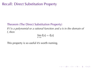
![Why a sum of continuous functions is continuous
We want to show that
lim (f + g)(x) = (f + g)(a).
x →a
We just follow our nose:
lim (f + g)(x) = lim [f(x) + g(x)] (def of f + g)
x →a x →a
= lim f(x) + lim g(x) (if these limits exist)
x →a x →a
= f(a) + g(a) (they do; f and g are cts.)
= (f + g)(a) (def of f + g again)
. . . . . .](https://image.slidesharecdn.com/lesson05-continuityslides-100205125006-phpapp01/85/Lesson-5-Continuity-19-320.jpg)
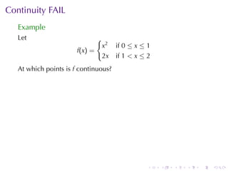
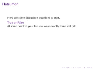
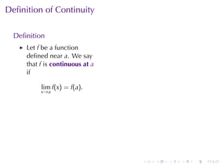
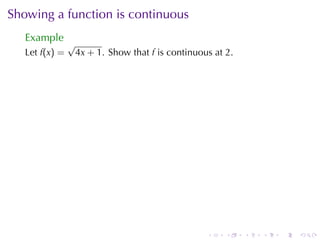
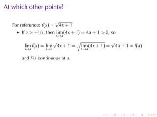
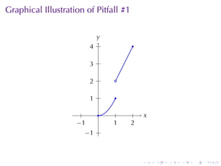
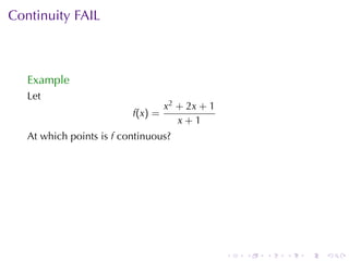
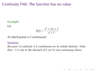
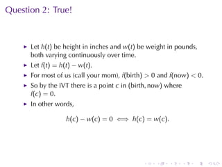
![Continuity FAIL: The limit does not exist
Example
Let {
x2 if 0 ≤ x ≤ 1
f(x ) =
2x if 1 < x ≤ 2
At which points is f continuous?
Solution
At any point a in [0, 2] besides 1, lim f(x) = f(a) because f is
x →a
represented by a polynomial near a, and polynomials have the
direct substitution property. However,
lim f(x) = lim x2 = 12 = 1
x →1 − x →1 −
lim f(x) = lim 2x = 2(1) = 2
x→1+ x →1 +
So f has no limit at 1. Therefore f is not continuous at 1.
. . . . . .](https://image.slidesharecdn.com/lesson05-continuityslides-100205125006-phpapp01/85/Lesson-5-Continuity-37-320.jpg)
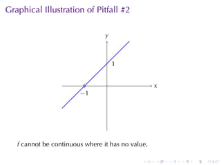
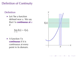
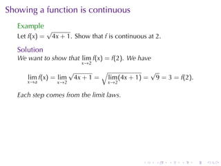
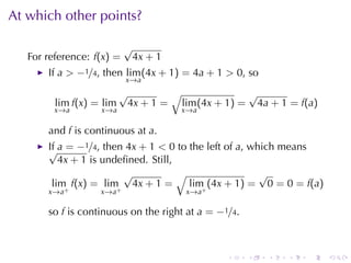
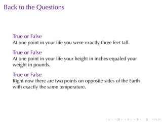
![The greatest integer function
[[x]] is the greatest integer ≤ x.
y
.
. .
3
x [[x]] y
. = [[x]]
0 0 . .
2 . .
1 1
1.5 1 . .
1 . .
1.9 1
2.1 2 . . . . . . x
.
−0.5 −1 −
. 2 −
. 1 1
. 2
. 3
.
−0.9 −1 .. 1 .
−
−1.1 −2
. .. 2 .
−
. . . . . .](https://image.slidesharecdn.com/lesson05-continuityslides-100205125006-phpapp01/85/Lesson-5-Continuity-53-320.jpg)
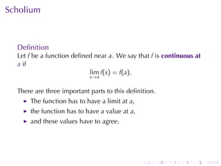
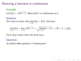
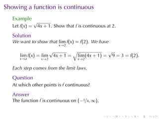
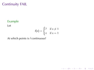
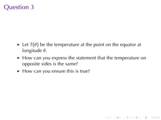
![The greatest integer function
[[x]] is the greatest integer ≤ x.
y
.
. .
3
x [[x]] y
. = [[x]]
0 0 . .
2 . .
1 1
1.5 1 . .
1 . .
1.9 1
2.1 2 . . . . . . x
.
−0.5 −1 −
. 2 −
. 1 1
. 2
. 3
.
−0.9 −1 .. 1 .
−
−1.1 −2
. .. 2 .
−
This function has a jump discontinuity at each integer.
. . . . . .](https://image.slidesharecdn.com/lesson05-continuityslides-100205125006-phpapp01/85/Lesson-5-Continuity-54-320.jpg)
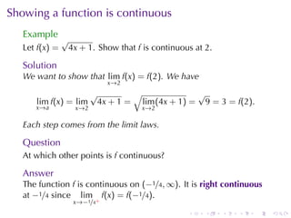
![A Big Time Theorem
Theorem (The Intermediate Value Theorem)
Suppose that f is continuous on the closed interval [a, b] and let N
be any number between f(a) and f(b), where f(a) ̸= f(b). Then
there exists a number c in (a, b) such that f(c) = N.
. . . . . .](https://image.slidesharecdn.com/lesson05-continuityslides-100205125006-phpapp01/85/Lesson-5-Continuity-56-320.jpg)

![Illustrating the IVT
Suppose that f is continuous on the closed interval [a, b]
f
.(x )
.
.
. x
.
. . . . . .](https://image.slidesharecdn.com/lesson05-continuityslides-100205125006-phpapp01/85/Lesson-5-Continuity-58-320.jpg)
![Illustrating the IVT
Suppose that f is continuous on the closed interval [a, b]
f
.(x )
f
.(b ) .
f
.(a ) .
. a
. x
.
b
.
. . . . . .](https://image.slidesharecdn.com/lesson05-continuityslides-100205125006-phpapp01/85/Lesson-5-Continuity-59-320.jpg)
![Illustrating the IVT
Suppose that f is continuous on the closed interval [a, b] and let N
be any number between f(a) and f(b), where f(a) ̸= f(b).
f
.(x )
f
.(b ) .
N
.
f
.(a ) .
. a
. x
.
b
.
. . . . . .](https://image.slidesharecdn.com/lesson05-continuityslides-100205125006-phpapp01/85/Lesson-5-Continuity-60-320.jpg)
![Illustrating the IVT
Suppose that f is continuous on the closed interval [a, b] and let N
be any number between f(a) and f(b), where f(a) ̸= f(b). Then
there exists a number c in (a, b) such that f(c) = N.
f
.(x )
f
.(b ) .
N
. .
f
.(a ) .
. a
. c
. x
.
b
.
. . . . . .](https://image.slidesharecdn.com/lesson05-continuityslides-100205125006-phpapp01/85/Lesson-5-Continuity-61-320.jpg)
![Illustrating the IVT
Suppose that f is continuous on the closed interval [a, b] and let N
be any number between f(a) and f(b), where f(a) ̸= f(b). Then
there exists a number c in (a, b) such that f(c) = N.
f
.(x )
f
.(b ) .
N
.
f
.(a ) .
. a
. x
.
b
.
. . . . . .](https://image.slidesharecdn.com/lesson05-continuityslides-100205125006-phpapp01/85/Lesson-5-Continuity-62-320.jpg)
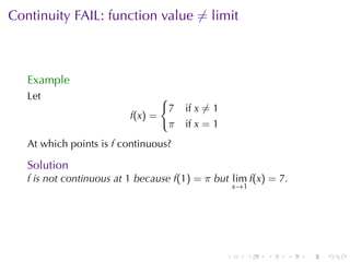
![Illustrating the IVT
Suppose that f is continuous on the closed interval [a, b] and let N
be any number between f(a) and f(b), where f(a) ̸= f(b). Then
there exists a number c in (a, b) such that f(c) = N.
f
.(x )
f
.(b ) .
N
. . . .
f
.(a ) .
. a c
. .1 x
.
c
.2 c b
.3 .
. . . . . .](https://image.slidesharecdn.com/lesson05-continuityslides-100205125006-phpapp01/85/Lesson-5-Continuity-63-320.jpg)

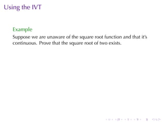
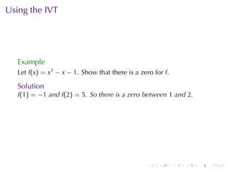
![Using the IVT
Example
Suppose we are unaware of the square root function and that it’s
continuous. Prove that the square root of two exists.
Proof.
Let f(x) = x2 , a continuous function on [1, 2].
. . . . . .](https://image.slidesharecdn.com/lesson05-continuityslides-100205125006-phpapp01/85/Lesson-5-Continuity-66-320.jpg)
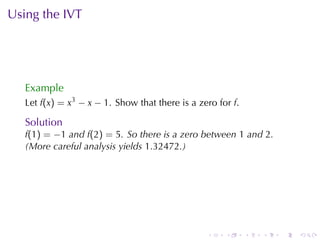
![Using the IVT
Example
Suppose we are unaware of the square root function and that it’s
continuous. Prove that the square root of two exists.
Proof.
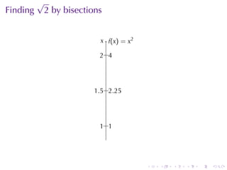
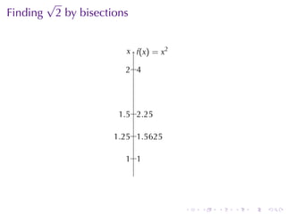
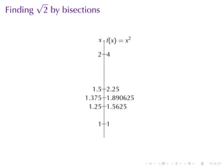
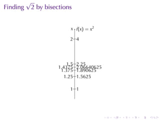
Let f(x) = x2 , a continuous function on [1, 2]. Note f(1) = 1 and
f(2) = 4. Since 2 is between 1 and 4, there exists a point c in
(1, 2) such that
f(c) = c2 = 2.
. . . . . .](https://image.slidesharecdn.com/lesson05-continuityslides-100205125006-phpapp01/85/Lesson-5-Continuity-67-320.jpg)
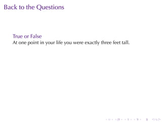
![Using the IVT
Example
Suppose we are unaware of the square root function and that it’s
continuous. Prove that the square root of two exists.
Proof.
Let f(x) = x2 , a continuous function on [1, 2]. Note f(1) = 1 and
f(2) = 4. Since 2 is between 1 and 4, there exists a point c in
(1, 2) such that
f(c) = c2 = 2.
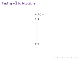
In fact, we can “narrow in” on the square root of 2 by the method
of bisections.
. . . . . .](https://image.slidesharecdn.com/lesson05-continuityslides-100205125006-phpapp01/85/Lesson-5-Continuity-68-320.jpg)


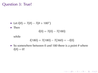


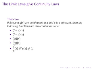
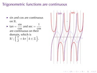
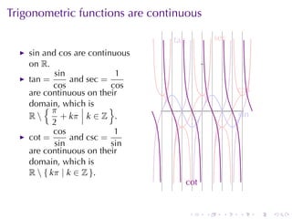
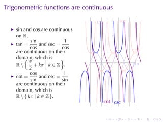
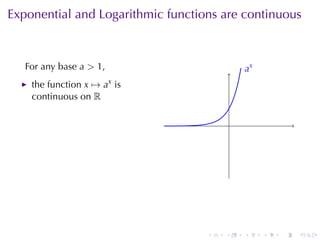
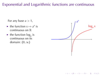
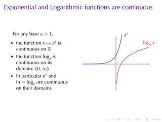
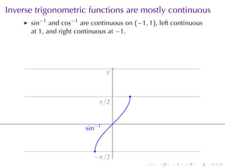
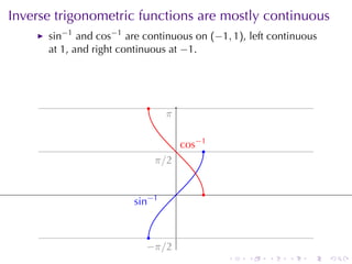
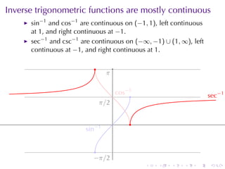
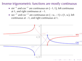
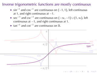
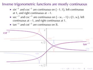
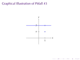
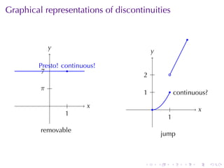
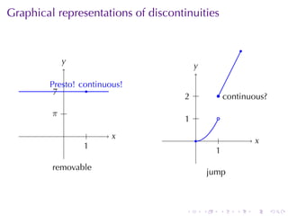
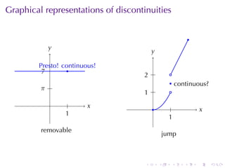
This document discusses the definition and properties of continuity in calculus, emphasizing the importance of limits and function values agreeing at a point. It includes examples of continuous functions and situations where continuity fails, along with types of discontinuities such as removable and jump discontinuities. Additionally, the text covers specific functions like polynomials, rational functions, trigonometric functions, and their continuity across different domains.


![Limits and continuity[1]](https://cdn.slidesharecdn.com/ss_thumbnails/limitsandcontinuity1-110816105053-phpapp01-thumbnail.jpg?width=640&height=640&fit=bounds)


