Download as PDF, PPTX


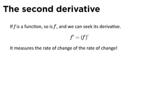
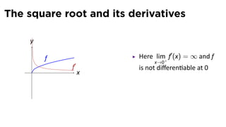


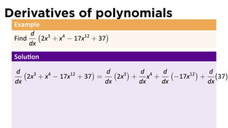
![Recall the Limit Laws
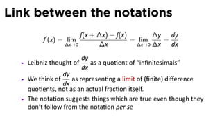
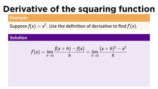
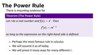
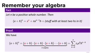
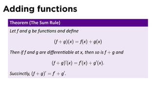
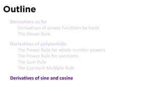
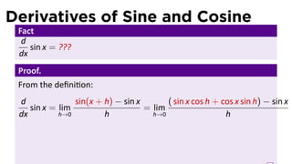
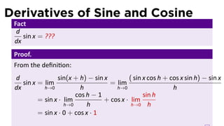
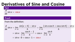
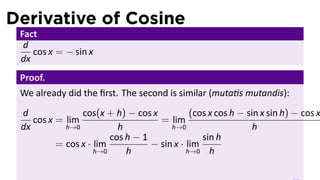
Fact
Suppose lim f(x) = L and lim g(x) = M and c is a constant. Then
x→a x→a
1. lim [f(x) + g(x)] = L + M
x→a
2. lim [f(x) − g(x)] = L − M
x→a
3. lim [cf(x)] = cL
x→a
4. . . .](https://image.slidesharecdn.com/lesson08-basicdifferentiationrules011slides-110219060329-phpapp02/85/Lesson-8-Basic-Differentation-Rules-slides-93-320.jpg)
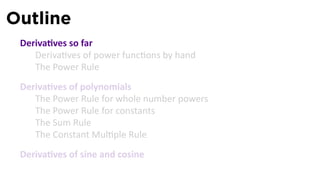
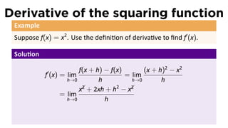
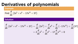
![Proof of the Sum Rule
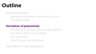
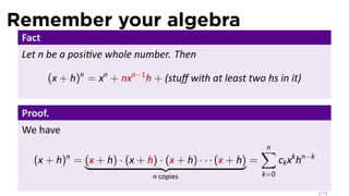
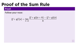
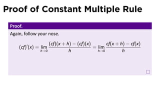
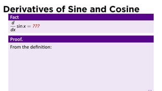
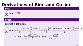
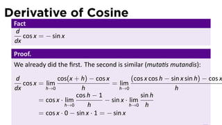
Proof.
Follow your nose:
(f + g)(x + h) − (f + g)(x)
(f + g)′ (x) = lim
h→0 h
f(x + h) + g(x + h) − [f(x) + g(x)]
= lim
h→0 h](https://image.slidesharecdn.com/lesson08-basicdifferentiationrules011slides-110219060329-phpapp02/85/Lesson-8-Basic-Differentation-Rules-slides-96-320.jpg)
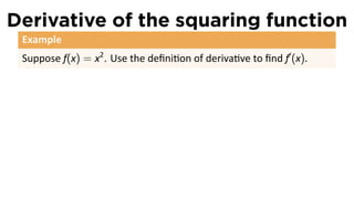
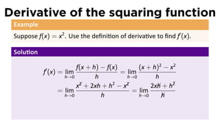
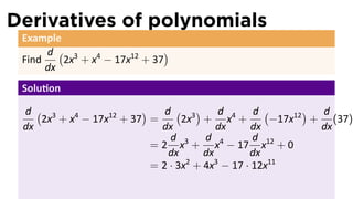
![Proof of the Sum Rule
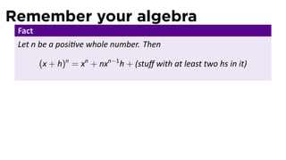
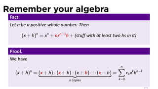
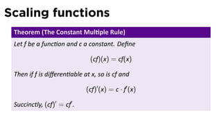
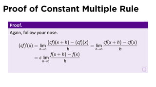
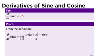
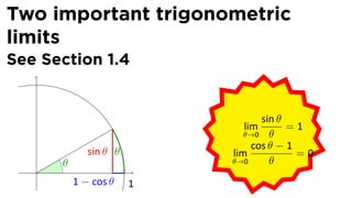
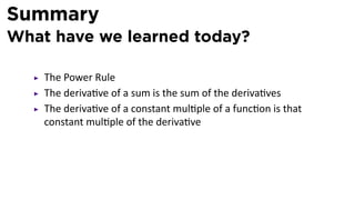
Proof.
Follow your nose:
(f + g)(x + h) − (f + g)(x)
(f + g)′ (x) = lim
h→0 h
f(x + h) + g(x + h) − [f(x) + g(x)]
= lim
h→0 h
f(x + h) − f(x) g(x + h) − g(x)
= lim + lim
h→0 h h→0 h](https://image.slidesharecdn.com/lesson08-basicdifferentiationrules011slides-110219060329-phpapp02/85/Lesson-8-Basic-Differentation-Rules-slides-97-320.jpg)
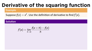
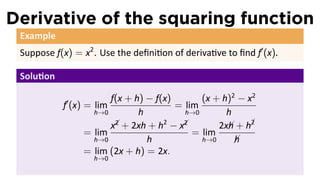
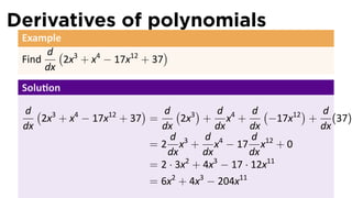
![Proof of the Sum Rule
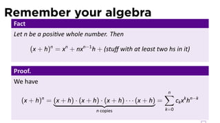
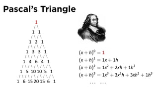
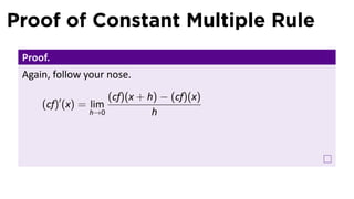
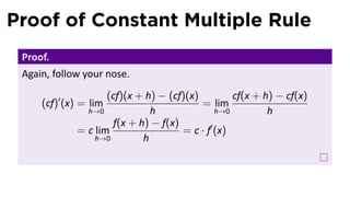
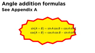
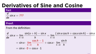
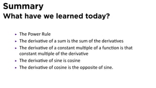
Proof.
Follow your nose:
(f + g)(x + h) − (f + g)(x)
(f + g)′ (x) = lim
h→0 h
f(x + h) + g(x + h) − [f(x) + g(x)]
= lim
h→0 h
f(x + h) − f(x) g(x + h) − g(x)
= lim + lim
h→0 h h→0 h
′ ′
= f (x) + g (x)](https://image.slidesharecdn.com/lesson08-basicdifferentiationrules011slides-110219060329-phpapp02/85/Lesson-8-Basic-Differentation-Rules-slides-98-320.jpg)
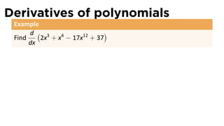
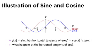
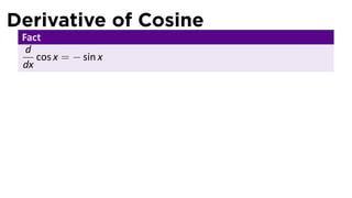
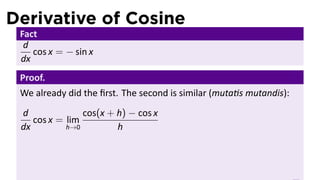
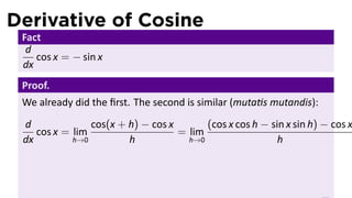


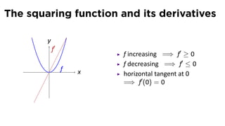
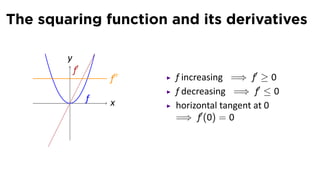
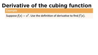
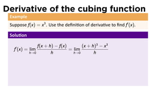
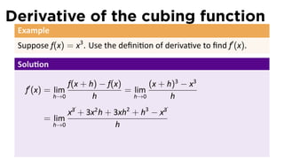
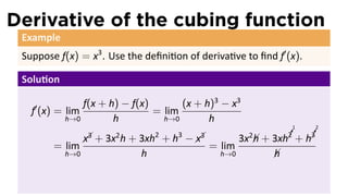
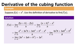
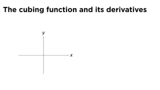
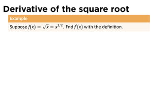
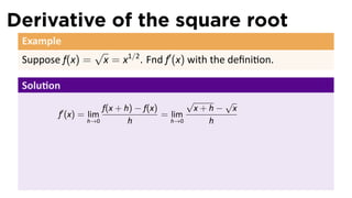
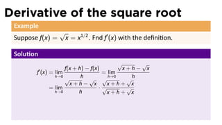
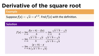
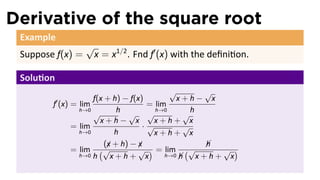
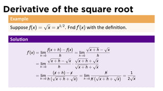
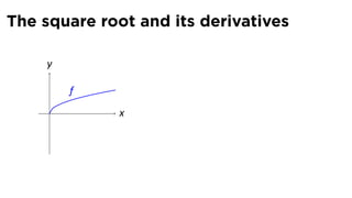
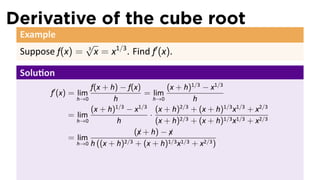
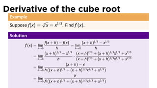
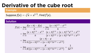
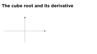
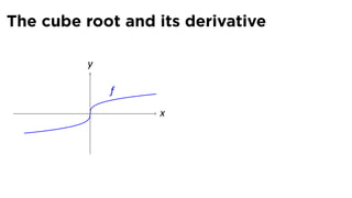
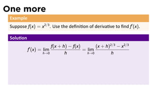
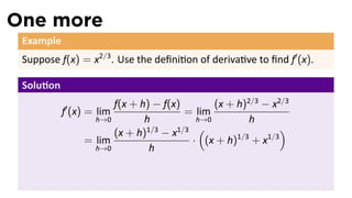
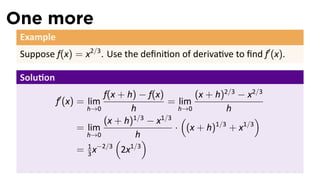
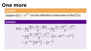
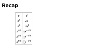
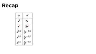
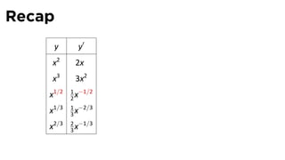
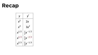
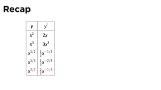
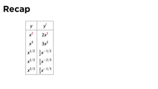
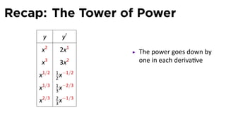
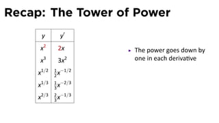
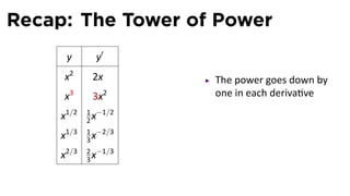
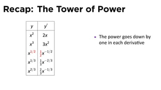
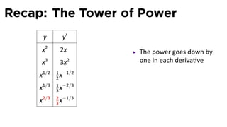
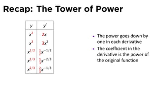
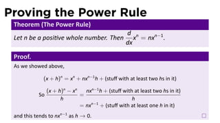
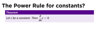
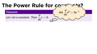
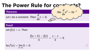
This document provides an outline for a calculus lecture on basic differentiation rules. It includes objectives to understand key rules like the constant multiple rule, sum rule, and derivatives of sine and cosine. Examples are worked through to find the derivatives of functions like squaring, cubing, square root, and cube root using the definition of the derivative. Graphs and properties of derived functions are also discussed.


