The document discusses the Mean Value Theorem (MVT) and Rolle's Theorem, providing their mathematical statements and proofs, as well as applications and examples. It outlines the importance of these theorems in understanding functions that are continuous and differentiable on certain intervals. Additionally, it addresses specific examples demonstrating the uniqueness of solutions to equations and the implications of theorems in real-world scenarios.

1. Sec on 4.2
The Mean Value Theorem
V63.0121.011: Calculus I
Professor Ma hew Leingang
New York University
April 6, 2011
.

2. Announcements
Quiz 4 on Sec ons 3.3,
3.4, 3.5, and 3.7 next
week (April 14/15)
Quiz 5 on Sec ons
4.1–4.4 April 28/29
Final Exam Thursday May
12, 2:00–3:50pm

3. Courant Lecture tomorrow
Persi Diaconis (Stanford)
“The Search for Randomness”
(General Audience Lecture)
Thursday, April 7, 2011, 3:30pm
Warren Weaver Hall, room 109
Recep on to follow
Visit http://cims.nyu.edu/ for details
and to RSVP

4. Objectives
Understand and be able
to explain the statement
of Rolle’s Theorem.
Understand and be able
to explain the statement
of the Mean Value
Theorem.

5. Outline
Rolle’s Theorem
The Mean Value Theorem
Applica ons
Why the MVT is the MITC
Func ons with deriva ves that are zero
MVT and differen ability

6. Heuristic Motivation for Rolle’s Theorem
If you bike up a hill, then back down, at some point your eleva on
was sta onary.
.
Image credit: SpringSun

7. Mathematical Statement of Rolle’s
Theorem
Theorem (Rolle’s Theorem)
Let f be con nuous on [a, b]
and differen able on (a, b).
Suppose f(a) = f(b). Then
there exists a point c in
(a, b) such that f′ (c) = 0. .
a b

8. Mathematical Statement of Rolle’s
Theorem
Theorem (Rolle’s Theorem)
c
Let f be con nuous on [a, b]
and differen able on (a, b).
Suppose f(a) = f(b). Then
there exists a point c in
(a, b) such that f′ (c) = 0. .
a b

9. Flowchart proof of Rolle’s Theorem
endpoints
Let c be
. Let d be
. . .
are max
the max pt the min pt
and min
f is
is c.an is d. an. .
yes yes constant
endpoint? endpoint?
on [a, b]
no no
′ ′ f′ (x) .≡ 0
f (c) .= 0 f (d) .= 0
on (a, b)

10. Outline
Rolle’s Theorem
The Mean Value Theorem
Applica ons
Why the MVT is the MITC
Func ons with deriva ves that are zero
MVT and differen ability

11. Heuristic Motivation for The Mean Value Theorem
If you drive between points A and B, at some me your speedometer
reading was the same as your average speed over the drive.
.
Image credit: ClintJCL

12. The Mean Value Theorem
Theorem (The Mean Value Theorem)
Let f be con nuous on
[a, b] and differen able on
(a, b). Then there exists a
point c in (a, b) such that
f(b) − f(a) b
= f′ (c). .
b−a a

13. The Mean Value Theorem
Theorem (The Mean Value Theorem)
Let f be con nuous on
[a, b] and differen able on
(a, b). Then there exists a
point c in (a, b) such that
f(b) − f(a) b
= f′ (c). .
b−a a

14. The Mean Value Theorem
Theorem (The Mean Value Theorem)
Let f be con nuous on c
[a, b] and differen able on
(a, b). Then there exists a
point c in (a, b) such that
f(b) − f(a) b
= f′ (c). .
b−a a

15. Rolle vs. MVT
f(b) − f(a)
f′ (c) = 0 = f′ (c)
b−a
c c
b
. .
a b a

16. Rolle vs. MVT
f(b) − f(a)
f′ (c) = 0 = f′ (c)
b−a
c c
b
. .
a b a
If the x-axis is skewed the pictures look the same.

17. Proof of the Mean Value Theorem
Proof.
The line connec ng (a, f(a)) and (b, f(b)) has equa on
f(b) − f(a)
L(x) = f(a) + (x − a)
b−a

18. Proof of the Mean Value Theorem
Proof.
The line connec ng (a, f(a)) and (b, f(b)) has equa on
f(b) − f(a)
L(x) = f(a) + (x − a)
b−a
Apply Rolle’s Theorem to the func on
f(b) − f(a)
g(x) = f(x) − L(x) = f(x) − f(a) − (x − a).
b−a

19. Proof of the Mean Value Theorem
Proof.
The line connec ng (a, f(a)) and (b, f(b)) has equa on
f(b) − f(a)
L(x) = f(a) + (x − a)
b−a
Apply Rolle’s Theorem to the func on
f(b) − f(a)
g(x) = f(x) − L(x) = f(x) − f(a) − (x − a).
b−a
Then g is con nuous on [a, b] and differen able on (a, b) since f is.

20. Proof of the Mean Value Theorem
Proof.
The line connec ng (a, f(a)) and (b, f(b)) has equa on
f(b) − f(a)
L(x) = f(a) + (x − a)
b−a
Apply Rolle’s Theorem to the func on
f(b) − f(a)
g(x) = f(x) − L(x) = f(x) − f(a) − (x − a).
b−a
Then g is con nuous on [a, b] and differen able on (a, b) since f is.
Also g(a) = 0 and g(b) = 0 (check both).

21. Proof of the Mean Value Theorem
Proof.
f(b) − f(a)
g(x) = f(x) − L(x) = f(x) − f(a) − (x − a).
b−a
So by Rolle’s Theorem there exists a point c in (a, b) such that
f(b) − f(a)
0 = g′ (c) = f′ (c) − .
b−a

22. Using the MVT to count solutions
Example
Show that there is a unique solu on to the equa on x3 − x = 100 in the
interval [4, 5].

23. Using the MVT to count solutions
Example
Show that there is a unique solu on to the equa on x3 − x = 100 in the
interval [4, 5].
Solu on
By the Intermediate Value Theorem, the func on f(x) = x3 − x
must take the value 100 at some point on c in (4, 5).

24. Using the MVT to count solutions
Example
Show that there is a unique solu on to the equa on x3 − x = 100 in the
interval [4, 5].
Solu on
By the Intermediate Value Theorem, the func on f(x) = x3 − x
must take the value 100 at some point on c in (4, 5).
If there were two points c1 and c2 with f(c1 ) = f(c2 ) = 100,
then somewhere between them would be a point c3 between
them with f′ (c3 ) = 0.

25. Using the MVT to count solutions
Example
Show that there is a unique solu on to the equa on x3 − x = 100 in the
interval [4, 5].
Solu on
By the Intermediate Value Theorem, the func on f(x) = x3 − x
must take the value 100 at some point on c in (4, 5).
If there were two points c1 and c2 with f(c1 ) = f(c2 ) = 100,
then somewhere between them would be a point c3 between
them with f′ (c3 ) = 0.
However, f′ (x) = 3x2 − 1, which is posi ve all along (4, 5). So
this is impossible.

26. Using the MVT to estimate
Example
We know that |sin x| ≤ 1 for all x, and that sin x ≈ x for small x.
Show that |sin x| ≤ |x| for all x.

27. Using the MVT to estimate
Example
We know that |sin x| ≤ 1 for all x, and that sin x ≈ x for small x.
Show that |sin x| ≤ |x| for all x.
Solu on
Apply the MVT to the func on
f(t) = sin t on [0, x]. We get Since |cos(c)| ≤ 1, we get
sin x − sin 0 sin x
= cos(c) ≤ 1 =⇒ |sin x| ≤ |x|
x−0 x
for some c in (0, x).

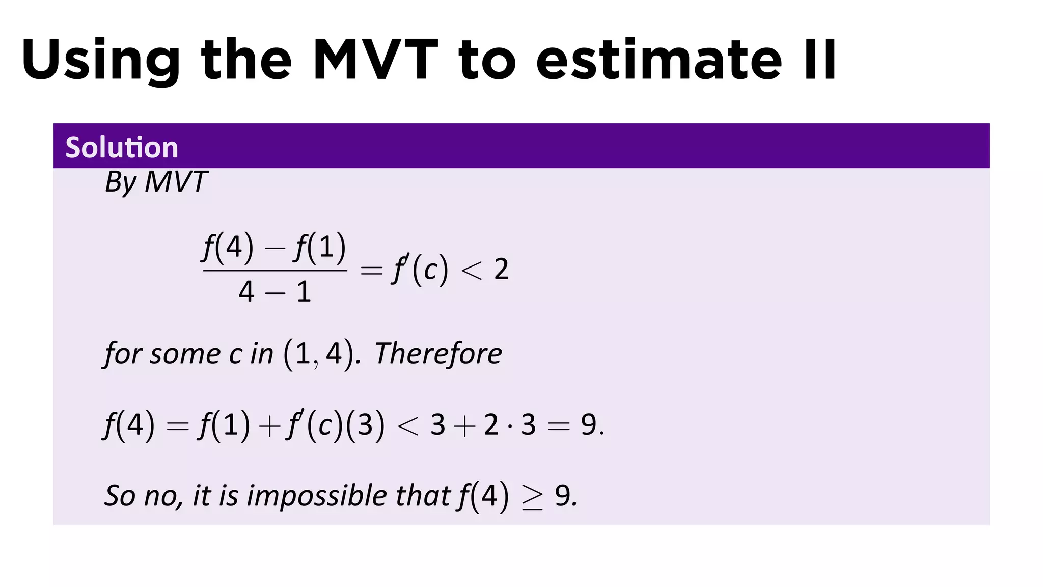
28. Using the MVT to estimate II
Example
Let f be a differen able func on with f(1) = 3 and f′ (x) < 2 for all x
in [0, 5]. Could f(4) ≥ 9?

29. Using the MVT to estimate II
Solu on
By MVT
f(4) − f(1)
= f′ (c) < 2
4−1
for some c in (1, 4). Therefore
f(4) = f(1) + f′ (c)(3) < 3 + 2 · 3 = 9.
So no, it is impossible that f(4) ≥ 9.

30. Using the MVT to estimate II
Solu on
By MVT
y (4, 9)
f(4) − f(1)
= f′ (c) < 2 (4, f(4))
4−1
for some c in (1, 4). Therefore
f(4) = f(1) + f′ (c)(3) < 3 + 2 · 3 = 9. (1, 3)
So no, it is impossible that f(4) ≥ 9. . x

31. Food for Thought
Ques on
A driver travels along the New Jersey Turnpike using E-ZPass. The
system takes note of the me and place the driver enters and exits
the Turnpike. A week a er his trip, the driver gets a speeding cket
in the mail. Which of the following best describes the situa on?
(a) E-ZPass cannot prove that the driver was speeding
(b) E-ZPass can prove that the driver was speeding
(c) The driver’s actual maximum speed exceeds his cketed speed
(d) Both (b) and (c).

32. Food for Thought
Ques on
A driver travels along the New Jersey Turnpike using E-ZPass. The
system takes note of the me and place the driver enters and exits
the Turnpike. A week a er his trip, the driver gets a speeding cket
in the mail. Which of the following best describes the situa on?
(a) E-ZPass cannot prove that the driver was speeding
(b) E-ZPass can prove that the driver was speeding
(c) The driver’s actual maximum speed exceeds his cketed speed
(d) Both (b) and (c).

33. Outline
Rolle’s Theorem
The Mean Value Theorem
Applica ons
Why the MVT is the MITC
Func ons with deriva ves that are zero
MVT and differen ability

34. Functions with derivatives that are zero
Fact
If f is constant on (a, b), then f′ (x) = 0 on (a, b).

35. Functions with derivatives that are zero
Fact
If f is constant on (a, b), then f′ (x) = 0 on (a, b).
The limit of difference quo ents must be 0
The tangent line to a line is that line, and a constant func on’s
graph is a horizontal line, which has slope 0.
Implied by the power rule since c = cx0

36. Functions with derivatives that are zero
Ques on
If f′ (x) = 0 is f necessarily a constant func on?

37. Functions with derivatives that are zero
Ques on
If f′ (x) = 0 is f necessarily a constant func on?
It seems true
But so far no theorem (that we have proven) uses informa on
about the deriva ve of a func on to determine informa on
about the func on itself

38. Why the MVT is the MITC
(Most Important Theorem In Calculus!)
Theorem
Let f′ = 0 on an interval (a, b).

39. Why the MVT is the MITC
(Most Important Theorem In Calculus!)
Theorem
Let f′ = 0 on an interval (a, b). Then f is constant on (a, b).

40. Why the MVT is the MITC
(Most Important Theorem In Calculus!)
Theorem
Let f′ = 0 on an interval (a, b). Then f is constant on (a, b).
Proof.
Pick any points x and y in (a, b) with x < y. Then f is con nuous on
[x, y] and differen able on (x, y). By MVT there exists a point z in
(x, y) such that
f(y) − f(x)
= f′ (z) = 0.
y−x
So f(y) = f(x). Since this is true for all x and y in (a, b), then f is
constant.

41. Functions with the same derivative
Theorem
Suppose f and g are two differen able func ons on (a, b) with
f′ = g′ . Then f and g differ by a constant. That is, there exists a
constant C such that f(x) = g(x) + C.

42. Functions with the same derivative
Theorem
Suppose f and g are two differen able func ons on (a, b) with
f′ = g′ . Then f and g differ by a constant. That is, there exists a
constant C such that f(x) = g(x) + C.
Proof.

43. Functions with the same derivative
Theorem
Suppose f and g are two differen able func ons on (a, b) with
f′ = g′ . Then f and g differ by a constant. That is, there exists a
constant C such that f(x) = g(x) + C.
Proof.
Let h(x) = f(x) − g(x)

44. Functions with the same derivative
Theorem
Suppose f and g are two differen able func ons on (a, b) with
f′ = g′ . Then f and g differ by a constant. That is, there exists a
constant C such that f(x) = g(x) + C.
Proof.
Let h(x) = f(x) − g(x)
Then h′ (x) = f′ (x) − g′ (x) = 0 on (a, b)

45. Functions with the same derivative
Theorem
Suppose f and g are two differen able func ons on (a, b) with
f′ = g′ . Then f and g differ by a constant. That is, there exists a
constant C such that f(x) = g(x) + C.
Proof.
Let h(x) = f(x) − g(x)
Then h′ (x) = f′ (x) − g′ (x) = 0 on (a, b)
So h(x) = C, a constant

46. Functions with the same derivative
Theorem
Suppose f and g are two differen able func ons on (a, b) with
f′ = g′ . Then f and g differ by a constant. That is, there exists a
constant C such that f(x) = g(x) + C.
Proof.
Let h(x) = f(x) − g(x)
Then h′ (x) = f′ (x) − g′ (x) = 0 on (a, b)
So h(x) = C, a constant
This means f(x) − g(x) = C on (a, b)

47. MVT and differentiability
Example
Let
{
−x if x ≤ 0
f(x) =
x2 if x ≥ 0
Is f differen able at 0?

48. MVT and differentiability
Example Solu on (from the defini on)
Let We have
{
−x if x ≤ 0 f(x) − f(0) −x
f(x) = lim− = lim− = −1
x2 if x ≥ 0 x→0 x−0 x→0 x
f(x) − f(0) x2
Is f differen able at 0? lim = lim+ = lim+ x = 0
x→0+ x−0 x→0 x x→0
Since these limits disagree, f is not
differen able at 0.

49. MVT and differentiability
Example Solu on (Sort of)
Let If x < 0, then f′ (x) = −1. If x > 0, then
{ f′ (x) = 2x. Since
−x if x ≤ 0
f(x) =
x2 if x ≥ 0 lim+ f′ (x) = 0 and lim− f′ (x) = −1,
x→0 x→0
Is f differen able at 0? the limit lim f′ (x) does not exist and so f is
x→0
not differen able at 0.

50. Why only “sort of”?
This solu on is valid but less f′ (x)
direct. y f(x)
We seem to be using the
following fact: If lim f′ (x) does
x→a
not exist, then f is not . x
differen able at a.
equivalently: If f is differen able
at a, then lim f′ (x) exists.
x→a
But this “fact” is not true!

51. Differentiable with discontinuous derivative
It is possible for a func on f to be differen able at a even if lim f′ (x)
x→a
does not exist.
Example
{
′ x2 sin(1/x) if x ̸= 0
Let f (x) = .
0 if x = 0
Then when x ̸= 0,
f′ (x) = 2x sin(1/x) + x2 cos(1/x)(−1/x2 ) = 2x sin(1/x) − cos(1/x),
which has no limit at 0.

52. Differentiable with discontinuous derivative
It is possible for a func on f to be differen able at a even if lim f′ (x)
x→a
does not exist.
Example
{
′ x2 sin(1/x) if x ̸= 0
Let f (x) = .
0 if x = 0
However,
′ f(x) − f(0) x2 sin(1/x)
f (0) = lim = lim = lim x sin(1/x) = 0
x→0 x−0 x→0 x x→0
So f′ (0) = 0. Hence f is differen able for all x, but f′ is not
con nuous at 0!

53. Differentiability FAIL
f(x) f′ (x)
. x . x
This func on is differen able But the deriva ve is not
at 0. con nuous at 0!

54. MVT to the rescue
Lemma
Suppose f is con nuous on [a, b] and lim+ f′ (x) = m. Then
x→a
f(x) − f(a)
lim+ = m.
x→a x−a

55. MVT to the rescue
Proof.
Choose x near a and greater than a. Then
f(x) − f(a)
= f′ (cx )
x−a
for some cx where a < cx < x. As x → a, cx → a as well, so:
f(x) − f(a)
lim+ = lim+ f′ (cx ) = lim+ f′ (x) = m.
x→a x−a x→a x→a

56. Using the MVT to find limits
Theorem
Suppose
lim f′ (x) = m1 and lim+ f′ (x) = m2
x→a− x→a
If m1 = m2 , then f is differen able at a. If m1 ̸= m2 , then f is not
differen able at a.

57. Using the MVT to find limits
Proof.
We know by the lemma that
f(x) − f(a)
lim− = lim− f′ (x)
x→a x−a x→a
f(x) − f(a)
lim+ = lim+ f′ (x)
x→a x−a x→a
The two-sided limit exists if (and only if) the two right-hand sides
agree.

58. Summary
Rolle’s Theorem: under suitable condi ons, func ons must
have cri cal points.
Mean Value Theorem: under suitable condi ons, func ons
must have an instantaneous rate of change equal to the
average rate of change.
A func on whose deriva ve is iden cally zero on an interval
must be constant on that interval.
E-ZPass is kinder than we realized.