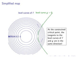
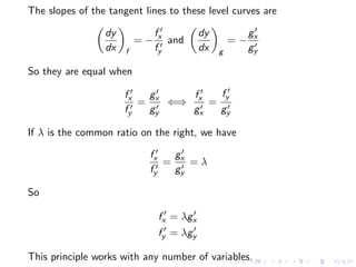
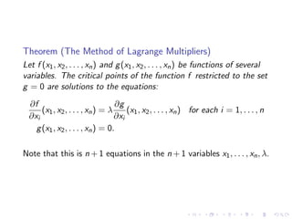
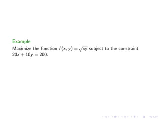
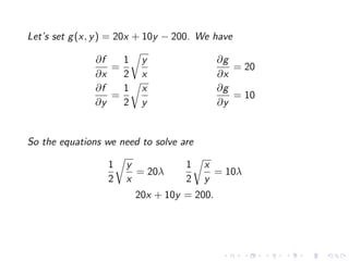
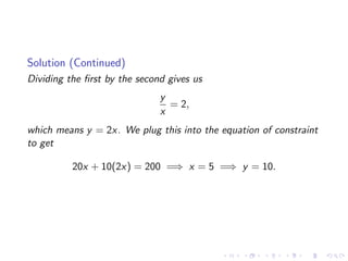
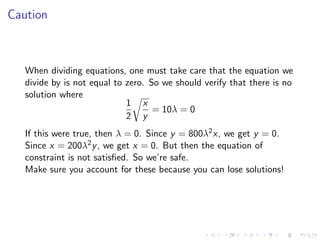
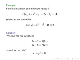
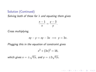
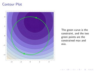
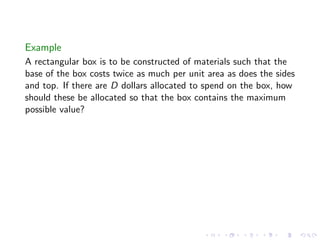
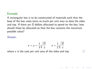
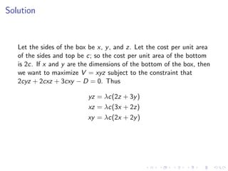
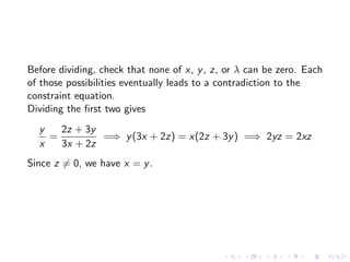
The document provides an overview of constrained optimization using Lagrange multipliers. It begins with motivational examples of constrained optimization problems and then introduces the method of Lagrange multipliers, which involves setting up equations involving the functions to optimize and constrain and a Lagrange multiplier. Examples are worked through to demonstrate solving these systems of equations to find critical points. Caution is advised about dividing equations where one side could be zero. A contour plot example visually depicts the constrained critical points.

1. Lesson 27 (Chapter 18.1–2)
Constrained Optimization I: Lagrange Multipliers
Math 20
November 26, 2007
Announcements
Problem Set 10 on the website. Due November 28.
next OH: Today 1–2, tomorrow 3–4 (SC 323)
Midterm II Review: Tuesday 12/4, 7:30–9:00pm in Hall E
Midterm II: Thursday, 12/6, 7–8:30pm in Hall A

2. Outline
Motivation
The Method of Lagrange Multipliers
Examples

3. The problem
We know how to find the critical points of a function of two
variables: look for where f = 0. That is,
∂f ∂f
= =0
∂x ∂y

4. The problem
We know how to find the critical points of a function of two
variables: look for where f = 0. That is,
∂f ∂f
= =0
∂x ∂y
Sometimes, however, we have a constraint which restricts us from
choosing variables freely:
Maximize volume subject to limited material costs
Minimize surface area subject to fixed volume
Maximize utility subject to limited income

5. Example
Maximize the function
√
f (x, y ) = xy
subject to the constraint
g (x, y ) = 20x + 10y = 200.

6. √
Maximize the function f (x, y ) = xy subject to the constraint
20x + 10y = 200.

7. √
Maximize the function f (x, y ) = xy subject to the constraint
20x + 10y = 200.
Solution
Solve the constraint for y and make f a single-variable function:
2x + y = 20, so y = 20 − 2x. Thus
x(20 − 2x) = 20x − 2x 2
f (x) =
10 − 2x
1
f (x) = √ (20 − 4x) = √ .
2 20x − 2x 2
2 20x − 2x
Then f (x) = 0 when 10 − 2x = 0, or x = 5. Since y = 20 − 2x,
√
y = 10. f (5, 10) = 50.

8. Checking maximality: Closed Interval Method
Cf. Section 9.3
Once the function is restricted to the line 20x + 10y = 200, we
can’t plug in negative numbers for f (x). Since
x(20 − 2x)
f (x) =
we have a restricted domain of 0 ≤ x ≤ 10. We only need to check
f on these two endpoints and its critical point to find the
√
maximum value. But f (0) = f (10) = 0 so f (5) = 50 is the
maximum value.

9. Checking maximality: First Derivative Test
Cf. Section 9.2
We have
10 − 2x
f (x) = √
20x − 2x 2
The denominator is always positive, so the fraction is positive
exactly when the numerator is positive. So f (x) < 0 if x < 5 and
f (x) > 0 if x > 5. This means f changes from increasing to
decreasing at 5. So 5 is the global maximum point.

10. Checking maximality: Second Derivative Test
Cf. Section 9.4
We have
100
f (x) = −
(20x − 2x 2 )3/2
So f (5) < 0, which means f has a local maximum at 5. Since
there are no other critical points, this is the global maximum.

11. Example
Find the maximum and minimum values of
f (x, y ) = x 2 + y 2 − 2x − 2y + 14.
subject to the constraint
g (x, y ) = x 2 + y 2 − 16 ≡ 0.

12. Example
Find the maximum and minimum values of
f (x, y ) = x 2 + y 2 − 2x − 2y + 14.
subject to the constraint
g (x, y ) = x 2 + y 2 − 16 ≡ 0.
This one’s harder. Solving for y in terms of x involves the square
root, of which there’s two choices.

13. Example
Find the maximum and minimum values of
f (x, y ) = x 2 + y 2 − 2x − 2y + 14.
subject to the constraint
g (x, y ) = x 2 + y 2 − 16 ≡ 0.
This one’s harder. Solving for y in terms of x involves the square
root, of which there’s two choices.
There’s a better way!

14. Outline
Motivation
The Method of Lagrange Multipliers
Examples

15. Consider a path that moves across a hilly terrain. Where are the
critical points of elevation along your path?

16. Simplified map
level curve g = 0
level curves of f
At the constrained
critical point, the
tangents to the
-10 -7 -5 -3-2 -1
-9 -6 -4
-8
level curves of f
and g are in the
same direction!

17. The slopes of the tangent lines to these level curves are
dy fx dy gx
=− =−
and
dx fy dx gy
f g
So they are equal when
fy
fx g f
= x ⇐⇒ x =
fy gy gx gy
If λ is the common ratio on the right, we have
fx g
= x =λ
fy gy
So
fx = λgx
fy = λgy
This principle works with any number of variables.

18. Theorem (The Method of Lagrange Multipliers)
Let f (x1 , x2 , . . . , xn ) and g (x1 , x2 , . . . , xn ) be functions of several
variables. The critical points of the function f restricted to the set
g = 0 are solutions to the equations:
∂f ∂g
(x1 , x2 , . . . , xn ) = λ (x1 , x2 , . . . , xn ) for each i = 1, . . . , n
∂xi ∂xi
g (x1 , x2 , . . . , xn ) = 0.
Note that this is n + 1 equations in the n + 1 variables x1 , . . . , xn , λ.

19. Outline
Motivation
The Method of Lagrange Multipliers
Examples

20. Example
√
Maximize the function f (x, y ) = xy subject to the constraint
20x + 10y = 200.

21. Let’s set g (x, y ) = 20x + 10y − 200. We have
∂f 1 y ∂g
= = 20
∂x 2 x ∂x
∂f 1 x ∂g
= = 10
∂y 2 y ∂y
So the equations we need to solve are
1 y 1 x
= 20λ = 10λ
2 x 2 y
20x + 10y = 200.

22. Solution (Continued)
Dividing the first by the second gives us
y
= 2,
x
which means y = 2x. We plug this into the equation of constraint
to get
20x + 10(2x) = 200 =⇒ x = 5 =⇒ y = 10.

23. Caution
When dividing equations, one must take care that the equation we
divide by is not equal to zero. So we should verify that there is no
solution where
1x
= 10λ = 0
2y
If this were true, then λ = 0. Since y = 800λ2 x, we get y = 0.
Since x = 200λ2 y , we get x = 0. But then the equation of
constraint is not satisfied. So we’re safe.
Make sure you account for these because you can lose solutions!

24. Example
Find the maximum and minimum values of
f (x, y ) = x 2 + y 2 − 2x − 6y + 14.
subject to the constraint
g (x, y ) = x 2 + y 2 − 16 ≡ 0.

25. Example
Find the maximum and minimum values of
f (x, y ) = x 2 + y 2 − 2x − 6y + 14.
subject to the constraint
g (x, y ) = x 2 + y 2 − 16 ≡ 0.
Solution
We have the two equations
2x − 2 = λ(2x)
2y − 6 = λ(2y ).
as well as the third
x 2 + y 2 = 16.

26. Solution (Continued)
Solving both of these for λ and equating them gives
x −1 y −3
= .
x y
Cross multiplying,
xy − y = xy − 3x =⇒ y = 3x.
Plugging this in the equation of constraint gives
x 2 + (3x)2 = 16,
which gives x = ± and y = ±3
8/5, 8/5.

27. Solution (Continued)
Looking at the function
f (x, y ) = x 2 + y 2 − 2x − 2y + 14
We see that
√
94 + 10 5
f −2 2/5, −6 2/5 =
5
is the maximum and
√
94 − 10 5
f2 2/5, 6 2/5 s=
5
is the minimum value of the constrained function.

28. Contour Plot
4
2
The green curve is the
constraint, and the two
0
green points are the
constrained max and
min.
2
4
4 2 0 2 4

29. Compare and Contrast
Elimination Lagrange Multipliers
solve, then differentiate differentiate, then solve
messier (usually) nicer (usually) equations
equations more equations
fewer equations adaptable to more than
adaptable to more than one constraint
one constraint second derivative test
second derivative test is (later) is harder
easier multipliers have
contextual meaning

30. Another argument for Lagrange multipliers
To find the critical points of f subject to the constraint that
g = 0, create the lagrangian
L = f (x1 , x2 , . . . , xn ) − λg (x1 , x2 , . . . , xn )
If L is restricted to the set g = 0, L = f and so the constrained
critical points are unconstrained critical points of L . So for each i,
∂L ∂f ∂g
= 0 =⇒ =λ .
∂xi ∂xi ∂xi
But also,
∂L
= 0 =⇒ g (x1 , x2 , . . . , xn ) = 0.
∂λ

31. Example
A rectangular box is to be constructed of materials such that the
base of the box costs twice as much per unit area as does the sides
and top. If there are D dollars allocated to spend on the box, how
should these be allocated so that the box contains the maximum
possible value?

32. Example
A rectangular box is to be constructed of materials such that the
base of the box costs twice as much per unit area as does the sides
and top. If there are D dollars allocated to spend on the box, how
should these be allocated so that the box contains the maximum
possible value?
Answer.
1D 1D
x =y = z=
3c 2c
where c is the cost per unit area of the sides and top.

33. Solution
Let the sides of the box be x, y , and z. Let the cost per unit area
of the sides and top be c; so the cost per unit area of the bottom
is 2c. If x and y are the dimensions of the bottom of the box, then
we want to maximize V = xyz subject to the constraint that
2cyz + 2cxz + 3cxy − D = 0. Thus
yz = λc(2z + 3y )
xz = λc(3x + 2z)
xy = λc(2x + 2y )

34. Before dividing, check that none of x, y , z, or λ can be zero. Each
of those possibilities eventually leads to a contradiction to the
constraint equation.
Dividing the first two gives
y 2z + 3y
= =⇒ y (3x + 2z) = x(2z + 3y ) =⇒ 2yz = 2xz
x 3x + 2z
Since z = 0, we have x = y .

35. The last equation now becomes x 2 = 4λcx. Dividing the second
equation by this gives
z 3x + 2z
=⇒ z = 3 x.
= 2
x 4x
Putting these into the equation of constraint we have
D = 3cxy + 2cyz + 2xz = 3cx 2 + 3cx 2 + 3cx 2 = 9cx 2 .
So
1 D 1 D
x =y = z=
3 c 2 c
It also follows that
x 1 D
λ= =
c3
4c 12

36. Interpretation of λ
Let V ∗ be the maximum volume found by solving the Lagrange
multiplier equations. Then
D3
1 D 1 D 1 D 1
V∗ = =
c3
3 c 3 c 2 c 18
Now
dV ∗ 31 D 1 D
= = =λ
3 12 c 3
dD 2 18 c
This is true in general; the multiplier is the derivative of the
extreme value with respect to the constraint.